Robust data-driven discovery of governing physical laws with error bars

Abstract

Discovering governing physical laws from noisy data is a grand challenge in many science and engineering research areas. We present a new approach to data-driven discovery of ordinary differential equations (ODEs) and partial differential equations (PDEs), in explicit or implicit form. We demonstrate our approach on a wide range of problems, including shallow water equations and Navier–Stokes equations. The key idea is to select candidate terms for the underlying equations using dimensional analysis, and to approximate the weights of the terms with error bars using our threshold sparse Bayesian regression. This new algorithm employs Bayesian inference to tune the hyperparameters automatically. Our approach is effective, robust and able to quantify uncertainties by providing an error bar for each discovered candidate equation. The effectiveness of our algorithm is demonstrated through a collection of classical ODEs and PDEs. Numerical experiments demonstrate the robustness of our algorithm with respect to noisy data and its ability to discover various candidate equations with error bars that represent the quantified uncertainties. Detailed comparisons with the sequential threshold least-squares algorithm and the lasso algorithm are studied from noisy time-series measurements and indicate that the proposed method provides more robust and accurate results. In addition, the data-driven prediction of dynamics with error bars using discovered governing physical laws is more accurate and robust than classical polynomial regressions.

1. Introduction

Almost all physical laws in nature are mathematical symmetries and invariants, suggesting that the search for many natural laws is a search for conservative properties and invariant equations [1–3]. In areas of science and engineering, the case is often encountered when the amount of experimental data is generous while the physical model is unclear. Discovering the governing physical laws behind noisy data is critical to the understanding of physical phenomena and prediction of future dynamics. Johannes Kepler published his three laws about planetary motion in the seventeenth century, having found them by analysing the astronomical observations of Tycho Brahe [4]. It took many years for Kepler to find the laws about planetary motion in the seventeenth century, but in recent years, the continuous growth of computing power with multiple-core processors makes the fast and automated physical-law discovery processes possible. Our goal is to design an automated physical-law discovery process, such that it can be applied to all kinds of datasets, to discover the physical laws that govern the dataset, where physical laws exist.

Suppose $f:{\mathbb{R}}^{d_1}\to {\mathbb{R}}^{d_2}$ is the governing function of some physical laws. Given dataset {x_i, f(x_i)}^N_i=0, interpolation or regression methods are available for the purpose of finding or approximating f. However, in some cases especially when f is in complicated or implicit form, interpolation or regression may have very poor results. From another perspective, we suggest a robust data-driven approach to discovering f in two steps. First, discover the differential equations satisfied by f; second, obtain the solution f, by solving the equations analytically or numerically. Besides having more flexibility to a larger class of functions than interpolation or regression, our approach derives the governing differential equations, which provide insights to the governing physical laws behind the observations.

Consider a dynamical system of the form

$$\frac{\mathrm{d}y}{\mathrm{d}x}=f(x,y).$$ 1.1

Given data {x_i, y_i, y′_i}^N_i=1, where y_i = y(x_i) and y′_i = (dy/dx)(x_i), we try to find the expression of f(x, y). A similar case was proposed in [5] and the related theories were further discussed in [6–16]. The method of data-driven discovery of dynamical systems has a wide range of applications, including biological networks [17], phenomenological dynamical models [18], parsimonious phenomenological models of cellular dynamics [19], predator–prey systems [20], stochastic dynamical systems [21] and optical fibre communications systems [22].

The following is a simple example of how this procedure works. First, we pick a set of basis-functions containing all the terms of f(x, y); for instance, {1, x, y, x², y², xy}. The set of basis-functions can have more terms than f(x, y), and we tend to pick a moderately large set to guarantee that all the terms of f(x, y) are contained. Then, algorithms are applied to search the subset of basis-functions that are exactly all the terms of f(x, y) and to determine the corresponding weights. Using the given noisy data and the basis-functions, we construct the following system

$$\left[\begin{array}{c}{y^{\mathrm{\prime }}}_1\\ {y^{\mathrm{\prime }}}_2\\ ⋮\\ {y^{\mathrm{\prime }}}_N\end{array}\right]=\left[\begin{array}{cccccc}1\hspace{0.17em}& x_1& y_1& x_1^2& y_1^2& x_1{y}_1\\ 1\hspace{0.17em}& x_2& y_2& x_2^2& y_2^2& x_2{y}_2\\ ⋮& ⋮& ⋮& ⋮& ⋮& ⋮\\ 1& x_N& y_N& x_N^2& y_N^2& x_N{y}_N\end{array}\right]\hspace{0.17em}\left[\begin{array}{c}{w}_1\\ w_2\\ w_3\\ w_4\\ w_5\\ w_6\end{array}\right]+\left[\begin{array}{c}{ϵ}_1\\ {ϵ}_2\\ ⋮\\ {ϵ}_N\end{array}\right],$$ 1.2

to find the weight-vector [w₁, w₂, w₃, w₄, w₅, w₆]^T, where [ϵ₁, ϵ₂, …, ϵ_N]^T is the model error. If the data were generated from dy/dx = x², an ideal algorithm should output the weight-vector [0, 0, 0, 1, 0, 0]^T. Note that many physical systems have few terms in the equations, which suggests the use of a sparse method. Denote η = [y′₁, …, y′_N]^T, $\mathrm{\Phi }=[{\varphi }_1,\dots ,{\varphi }_6]=\left[\begin{array}{ccc}1& \dots & x_1{y}_1\\ ⋮& \ddots & ⋮\\ 1& \dots & x_N{y}_N\end{array}\right]$, w = [w₁, …, w₆]^T and ϵ = [ϵ₁, …, ϵ_N]^T. Finding the weight-vector w is equivalent to solving the sparse regression problem

$$\eta =\mathrm{\Phi }\mathbf{w}+ϵ,$$ 1.3

where η, Φ are known, ϵ is the model error and w is to be determined sparsely. To solve this problem, one may use sequential threshold least squares [5], which does least-square regression and eliminates the terms with small weights iteratively, or may use lasso [6,23]. In this paper, we use threshold sparse Bayesian regression algorithm, which is a modification of RVM (relevance vector machine [24,25]). Similar sparse methods are also popular in compressive sensing [26–30] and dictionary learning [31,32]. Compared to the other sparse methods, our algorithm takes advantage of Bayesian inference to provide error bars and to quantify uncertainties in the data-driven discovery process.

The remainder of this paper is structured as follows. In §2, we introduce a general discovery pattern for discovering governing physical laws. In §3, we propose an algorithm for sparse regression based on RVM. Some numerical examples are presented in §4, followed in §5 by a conclusion.

2. General discovery pattern

Discovering governing differential equations in a pattern like (1.1) is limited: this algorithm needs some prior knowledge of the equation to discover it. In other words, the term on the left-hand side of the equation must be known before the algorithm tries to discover the equation. For example, if written in the form

$$\frac{\mathrm{d}y}{\mathrm{d}x}=f(x,y),$$ 2.1

then the differential equation must contain the term dy/dx, and other terms are of order less than 1. If written in the form

$$\frac{{\mathrm{d}}^{2}y}{\mathrm{d}{x}^2}=f(x,y,\frac{\mathrm{d}y}{\mathrm{d}x}),$$ 2.2

then the differential equation must contain the term d²y/dx², and other terms are of order less than 2. More complicated physical systems in implicit form, such as Laguerre differential equation

$$x\frac{{\mathrm{d}}^{2}y}{\mathrm{d}{x}^2}+(1-x)\frac{\mathrm{d}y}{\mathrm{d}x}=0,$$ 2.3

cannot be written in (2.1), (2.2), or similar forms of higher order. When we are given just the data, but not given what term the equation must contain, we can use the following method to discover the differential equation.

Firstly, when higher-order derivatives are present in the governing physical laws, a set of basis-functions is chosen to contain these higher-order derivatives, such as

$$\stackrel{d}{⨂}\{1,x,y,\frac{\mathrm{d}y}{\mathrm{d}x},\frac{{\mathrm{d}}^{2}y}{\mathrm{d}{x}^2},\dots ,\frac{{\mathrm{d}}^{k}y}{\mathrm{d}{x}^k}\},$$ 2.4

where d, k are positive integers and $\stackrel{d}{⨂}S$ denotes ‘tensor product’ of d copies of set S. For example, when d = 1 and k = 1, the basis is

$$\{1,x,y,\frac{\mathrm{d}y}{\mathrm{d}x}\};$$ 2.5

when d = 1 and k = 2, the basis is

$$\{1,x,y,\frac{\mathrm{d}y}{\mathrm{d}x},\frac{{\mathrm{d}}^{2}y}{\mathrm{d}{x}^2}\};$$ 2.6

when d = 2 and k = 1, the basis is

$$\{1,x,y,\frac{\mathrm{d}y}{\mathrm{d}x},x^2,xy,x\frac{\mathrm{d}y}{\mathrm{d}x},y^2,y\frac{\mathrm{d}y}{\mathrm{d}x},{\left(\frac{\mathrm{d}y}{\mathrm{d}x}\right)}^2\};$$ 2.7

when d = 2 and k = 2, the basis is

$$\{1,x,y,\frac{\mathrm{d}y}{\mathrm{d}x},\frac{{\mathrm{d}}^{2}y}{\mathrm{d}{x}^2},x^2,xy,x\frac{\mathrm{d}y}{\mathrm{d}x},x\frac{{\mathrm{d}}^{2}y}{\mathrm{d}{x}^2},y^2,y\frac{dy}{dx},y\frac{{\mathrm{d}}^{2}y}{\mathrm{d}{x}^2},{\left(\frac{\mathrm{d}y}{\mathrm{d}x}\right)}^2,\frac{\mathrm{d}y}{\mathrm{d}x}\frac{{\mathrm{d}}^{2}y}{\mathrm{d}{x}^2},{\left(\frac{{\mathrm{d}}^{2}y}{\mathrm{d}{x}^2}\right)}^2\}.$$ 2.8

The set of basis-functions constructed by ‘tensor product’ has $\frac{(d+k+2)!}{d!(k+2)!}$ elements, and grows very fast when d, k are large. Therefore, if additional knowledge about the physical system is available, some basis-functions that are certainly not part of the physical system should be eliminated beforehand. In addition, integers d, k may be increased adaptively to search different sets of basis-functions in sequence starting from lower-order ones. When the error bar is smaller than a preassigned value, the procedure is stopped and the governing physical laws are discovered.

Write the basis-functions into a vector

$$\mathbf{f}=[f_1(x,y,y^{\prime },\dots ,y^{(k)}),\dots ,f_M(x,y,y^{\prime },\dots ,y^{(k)})].$$ 2.9

Now the problem is to find a sparse weight-vector w = [w₁, …, w_M]^T satisfying

$$0=\mathbf{f}\mathbf{w}.$$ 2.10

A non-convex algorithm using alternating directions to find the sparse non-trivial solution w is analysed in [33], and a similar approach is used for discovering dynamical systems in [17]. They solve the sparse regression problem but without analysis of the uncertainty. Our approach solves the sparse regression problem using Bayesian inference and provides error bars that quantify the uncertainty of the discovered weights. After collecting the data

$${\mathbf{F}}_{ij}=f_j(x_i,y_i,y_i^{\prime },\dots ,y_i^{(k)}),$$ 2.11

we have the following sparse regression problem

$$\mathbf{0}=\mathbf{F}\mathbf{w}+ϵ,$$ 2.12

where ϵ is the model error. If sparse regression is performed in (2.12), the resulting weights may collapse to all zeros. As a result, we fix one of the weights to be 1 at a time and perform sparse regressions repeatedly for different fixed weights. Specifically, for each j∈{1, …, M}, fix w_j = 1 and solve the other weights in the following regression problem:

$$\mathbf{0}=\left[\begin{array}{cccc}{\mathbf{F}}_{11}& {\mathbf{F}}_{12}& \cdots & {\mathbf{F}}_{1M}\\ {\mathbf{F}}_{21}& {\mathbf{F}}_{22}& \cdots & {\mathbf{F}}_{2M}\\ ⋮& ⋮& \ddots & ⋮\\ {\mathbf{F}}_{N1}& {\mathbf{F}}_{N2}& \cdots & {\mathbf{F}}_{NM}\end{array}\right]\hspace{0.17em}\left[\begin{array}{c}{w}_1\\ ⋮\\ w_{j-1}\\ 1\\ w_{j+1}\\ ⋮\\ w_M\end{array}\right]+ϵ,$$ 2.13

which is equivalent to

$$\left[\begin{array}{c}{\mathbf{F}}_{1j}\\ {\mathbf{F}}_{2j}\\ ⋮\\ {\mathbf{F}}_{Nj}\end{array}\right]=-\left[\begin{array}{cccccc}{\mathbf{F}}_{11}& \cdots & {\mathbf{F}}_{1,j-1}& {\mathbf{F}}_{1,j+1}& \cdots & {\mathbf{F}}_{1M}\\ {\mathbf{F}}_{21}& \cdots & {\mathbf{F}}_{2,j-1}& {\mathbf{F}}_{2,j+1}& \cdots & {\mathbf{F}}_{2M}\\ ⋮& \ddots & ⋮& ⋮& \ddots & ⋮\\ {\mathbf{F}}_{N1}& \cdots & {\mathbf{F}}_{N,j-1}& {\mathbf{F}}_{N,j+1}& \cdots & {\mathbf{F}}_{NM}\end{array}\right]\hspace{0.17em}\left[\begin{array}{c}{w}_1\\ ⋮\\ w_{j-1}\\ w_{j+1}\\ ⋮\\ w_M\end{array}\right]-ϵ.$$ 2.14

Using the sparse regression method detailed in §3, we get the weights

$${[{\hat{w}}_1,\dots ,{\hat{w}}_{j-1},{\hat{w}}_{j+1},\dots ,{\hat{w}}_M]}^{\mathrm{T}},$$ 2.15

which indicate that the physical system might be

$$f_j=-{[f_1,\dots ,f_{j-1},f_{j+1},\dots ,f_M][{\hat{w}}_1,\dots ,{\hat{w}}_{j-1},{\hat{w}}_{j+1},\dots ,{\hat{w}}_M]}^{\mathrm{T}}$$ 2.16

or

$$0=\mathbf{f}\hat{\mathbf{w}},$$ 2.17

where $\hat{\mathbf{w}}={[{\hat{w}}_1,\dots ,{\hat{w}}_{j-1},1,{\hat{w}}_{j+1},\dots ,{\hat{w}}_M]}^{\mathrm{T}}$. If the real w_j≠0, the whole real equation can be multiplied by a constant such that w_j = 1, and the preceding procedure can discover the real equation. Now w_j may be 0, but at least one component of w is non-zero (otherwise the equation is 0 = 0). Thus, we perform the sparse regressions multiple times by fixing different components of w as 1, and compare the error bars obtained from different sparse regressions to select the best candidate equation. Here, at most M regressions are performed for j = 1, 2, …, M.

(a). Construct basis-functions of the same dimension

Using the basis-functions generating the technique introduced above, we constructed basis-functions by tensor-products. Owing to the rapid growth of the size of the tensor-products, the set of basis-functions can become very large, which may result in linear correlation within the basis-functions and therefore is bad for the accuracy of the result. What simplifies the case is that real-world data usually have dimensions, so do the basis-functions calculated by the data. Any physically meaningful equation has the same dimensions on every term, which is a property known as dimensional homogeneity [34]. Therefore, when summing up terms in the equations, the addends should be of the same dimension. For example, if we want to discover the relationship between force F and the second-order tensor generated by mass m and acceleration a, namely {1, m, a, m², a², ma}, then the only basis-function in the tensor having the same dimension as F is ma. Thus, we can use the following regression to discover the physical law

$$F=wma,$$ 2.18

where w is the weight to be estimated.

Following this rule, basis-functions of the same dimension are chosen as a set of basis-functions in the equation discovery process, which reduces the number of basis-functions efficiently and improves the performance of the algorithm significantly. More examples are listed in §4 in the discovery of shallow water equations and Navier–Stokes equations.

3. Threshold sparse Bayesian regression

To solve the sparse regression problem (2.14), we design an algorithm in this section. Note that all the F_ij in (2.14) can be calculated using the data by (2.11). Now, to describe our algorithm in a general setting, given noisy data, let η be a known vector calculated by the data, Φ be a known matrix calculated by the data, w = [w₁, w₂, …, w_M]^T be the weight-vector to be estimated sparsely, and ϵ be the model error:

$$\eta =\mathrm{\Phi }\mathbf{w}+ϵ.$$ 3.1

Sparse Bayesian inference assumes that the model errors are modelled as independent and identically distributed zero-mean Gaussian with variance σ², which may be specified beforehand, but in this paper it is fitted by the data. The model gives a multivariate Gaussian likelihood on the vector η:

$$p(\eta \hspace{0.17em}|\hspace{0.17em}\mathbf{w},{\sigma }^2)={(2\pi {\sigma }^2)}^{-N/2}\exp \{-\frac{\parallel \eta -\mathrm{\Phi }\mathbf{w}{\parallel }^2}{2{\sigma }^2}\}.$$ 3.2

The likelihood is coded with a Gaussian prior over the weights

$$p(\mathbf{w}|\alpha )=\prod _{j=1}^M\mathcal{N}(w_j\hspace{0.17em}|\hspace{0.17em}0,{\alpha }_j^{-1}),$$ 3.3

where α = [α₁, …, α_M]^T. Each α_j controls each w_j individually, which encourages the sparsity property of this model [24]. To complete the hierarchical model, we define hyperprior distributions over α as well as σ², the variance of the error. As these quantities are instances of the scale parameters [35], Gamma distributions are suitable:

$$p(\alpha )=\prod _{j=1}^M\mathrm{\Gamma }({\alpha }_j\hspace{0.17em}|\hspace{0.17em}a,b)$$ 3.4

and

$$p(\beta )=\mathrm{\Gamma }(\beta \hspace{0.17em}|\hspace{0.17em}c,d),$$ 3.5

with $\beta \triangleq {\sigma }^{-2}$, where a, b, c, d are constants. The sparse Bayesian model is specified by (3.2)–(3.5). See figure 1 for the graphical structure of this model.

Figure 1.

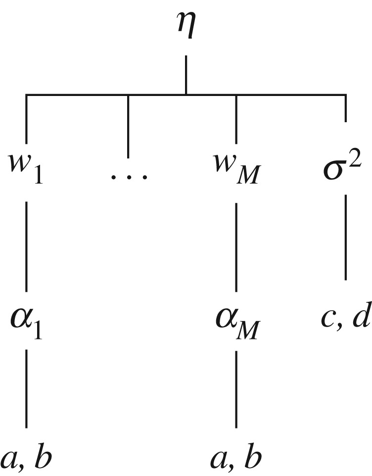
Graphical structure of the sparse Bayesian model.

The posterior over all unknown parameters given the data can be decomposed as follows:

$$p(\mathbf{w},\alpha ,{\sigma }^2|\eta )=p(\mathbf{w}\hspace{0.17em}|\hspace{0.17em}\eta ,\alpha ,{\sigma }^2)p(\alpha ,{\sigma }^2\hspace{0.17em}|\hspace{0.17em}\eta ).$$ 3.6

If assuming uniform scale priors on α and β with a = b = c = d = 0, we may approximate p(α, σ²|η) using Dirac delta function at $({\hat{\alpha }}_{ML},{\hat{\sigma }}_{ML}^2)$:

$$p(\mathbf{w},\alpha ,{\sigma }^2|\eta )\approx p(\mathbf{w}\hspace{0.17em}|\hspace{0.17em}\eta ,\alpha ,{\sigma }^2)\delta ({\hat{\alpha }}_{ML},{\hat{\sigma }}_{ML}^2),$$ 3.7

where

$$\begin{array}{rl}({\hat{\alpha }}_{ML},{\hat{\sigma }}_{ML}^2)& =\arg \underset{\alpha ,{\sigma }^2}{max}\{p(\eta \hspace{0.17em}|\hspace{0.17em}\alpha ,{\sigma }^2)\}\\ & =\arg \underset{\alpha ,{\sigma }^2}{max}\{\int p(\eta \hspace{0.17em}|\hspace{0.17em}\mathbf{w},{\sigma }^2)p(\mathbf{w}\hspace{0.17em}|\hspace{0.17em}\alpha )\hspace{0.17em}\mathrm{d}\mathbf{w}\}\\ & =\arg \underset{\alpha ,{\sigma }^2}{max}\{{(2\pi )}^{-N/2}|{\sigma }^2\mathbf{I}+\mathrm{\Phi }{\mathbf{A}}^{-1}{\mathrm{\Phi }}^{\mathrm{T}}{|}^{-1/2}\exp \{-\frac{1}{2}{\eta }^{\mathrm{T}}{({\sigma }^2\mathbf{I}+\mathrm{\Phi }{\mathbf{A}}^{-1}{\mathrm{\Phi }}^{\mathrm{T}})}^{-1}\eta \}\},\end{array}$$ 3.8

with A = diag(α₁, …, α_M). This maximization is known as the type-2 maximum-likelihood [35] and can be calculated using a fast method [36]. Now, we can integrate out α and σ² to get the posterior over the weights given data:

$$\begin{array}{rl}p(\mathbf{w}\hspace{0.17em}|\hspace{0.17em}\eta )& =\iint p(\mathbf{w},\alpha ,{\sigma }^2\hspace{0.17em}|\hspace{0.17em}\eta )\hspace{0.17em}\mathrm{d}\alpha \hspace{0.17em}\mathrm{d}{\sigma }^2\\ & \approx \iint p(\mathbf{w}\hspace{0.17em}|\hspace{0.17em}\eta ,\alpha ,{\sigma }^2)\delta ({\hat{\alpha }}_{ML},{\hat{\sigma }}_{ML}^2)\hspace{0.17em}\mathrm{d}\alpha \hspace{0.17em}\mathrm{d}{\sigma }^2\\ & =p(\mathbf{w}\hspace{0.17em}|\hspace{0.17em}\eta ,{\hat{\alpha }}_{ML},{\hat{\sigma }}_{ML}^2)\\ & =\frac{p(\eta \hspace{0.17em}|\hspace{0.17em}\mathbf{w},{\hat{\sigma }}_{ML}^2)p(\mathbf{w}\hspace{0.17em}|\hspace{0.17em}{\hat{\alpha }}_{ML})}{p(\eta \hspace{0.17em}|\hspace{0.17em}{\hat{\alpha }}_{ML},{\hat{\sigma }}_{ML}^2)}\\ & ={(2\pi )}^{-M/2}|\hat{\mathrm{\Sigma }}{|}^{-1/2}\exp \{-\frac{1}{2}{(\mathbf{w}-\hat{\mu })}^{\mathrm{T}}{\hat{\mathrm{\Sigma }}}^{-1}(\mathbf{w}-\hat{\mu })\}\\ & =\mathcal{N}(\mathbf{w}\hspace{0.17em}|\hspace{0.17em}\hat{\mu },\hat{\mathrm{\Sigma }}),\end{array}$$ 3.9

in which the posterior covariance and mean are as follows:

$$\hat{\mathrm{\Sigma }}={[{\hat{\sigma }}_{ML}^{-2}{\mathrm{\Phi }}^{\mathrm{T}}\mathrm{\Phi }+\mathrm{diag}({\hat{\alpha }}_{ML})]}^{-1}$$ 3.10

and

$$\hat{\mu }={\hat{\sigma }}_{ML}^{-2}\hat{\mathrm{\Sigma }}{\mathrm{\Phi }}^{\mathrm{T}}\eta .$$ 3.11

The optimal values of many of the hyperparameters α_j in (3.8) are infinite [24], which from (3.10) and (3.11) leads to a posterior with many weights w_j infinitely peaked at zero and results in the sparsity of the model.

The posterior for each weight can be deduced by (3.9) the following:

$$p(w_j\hspace{0.17em}|\hspace{0.17em}\eta )=\mathcal{N}(w_j\hspace{0.17em}|\hspace{0.17em}{\hat{\mu }}_j,{\hat{\mathrm{\Sigma }}}_{jj}),$$ 3.12

with mean ${\hat{\mu }}_j$ and standard deviation ${\hat{\mathrm{\Sigma }}}_{jj}^{1/2}$. To encourage accuracy and robustness, we place a threshold δ≥0 on the model to clean up possible disturbances present in the weight-vector and then reestimate the weight-vector using the remaining terms, iteratively until convergence. The entire procedure is summarized in algorithm 1. A discussion about how to choose the threshold is detailed in example f in §4.

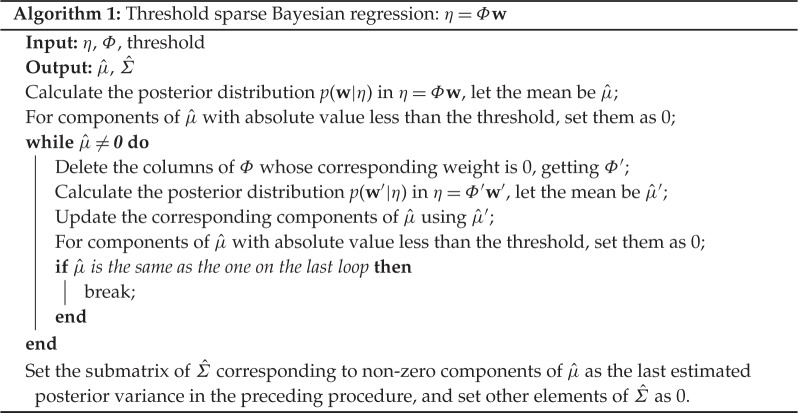
The error bar for the sparse regression (algorithm 1) is constructed as follows:

$$\mathrm{Errorbar}=\sum _{\begin{array}{c}j=1\\ {\hat{\mu }}_j\ne 0\end{array}}^M\frac{{\hat{\mathrm{\Sigma }}}_{jj}}{{\hat{\mu }}_j^2}.$$ 3.13

We divide ${\hat{\mathrm{\Sigma }}}_{jj}$ by ${\hat{\mu }}_j^2$ to normalize the uncertainty on each weight. In this construction, smaller error bars mean higher posterior confidence. Algorithm 1 is designed such that $\hat{\mu }$ has more 0 components after each loop. Therefore, its convergence is guaranteed given the convergence of calculation of the maximum likelihood in (3.8).

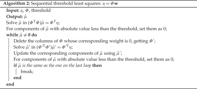
The method of sequential threshold least squares is summarized in algorithm 2, which is almost the same as ‘SINDy’ in [5]. The difference is that algorithm 2 does least squares iteratively until convergence while ‘SINDy’ in [5] caps the maximum number of loops as 10. The sufficient conditions of ‘SINDy’ for general convergence, rate of convergence and conditions for one-step recovery appear in [16]. In addition, the method of lasso [23] is summarized in algorithm 3.

4. Numerical results

(a). Comparison with sequential threshold least squares and lasso

Consider the two-dimensional dynamical system

$$\begin{array}{rl}\frac{\mathrm{d}{x}_1}{\mathrm{d}t}& =-0.5x_1+2x_2\\ \mathrm{and}\frac{\mathrm{d}{x}_2}{\mathrm{d}t}& =-2x_1-0.5x_2,\end{array}\}$$ 4.1

with the model

$$\begin{array}{rl}\frac{\mathrm{d}{x}_1}{\mathrm{d}t}& =\mathbf{f}{\mathbf{w}}_1\\ \mathrm{and}\frac{\mathrm{d}{x}_2}{\mathrm{d}t}& =\mathbf{f}{\mathbf{w}}_2,\end{array}\}$$ 4.2

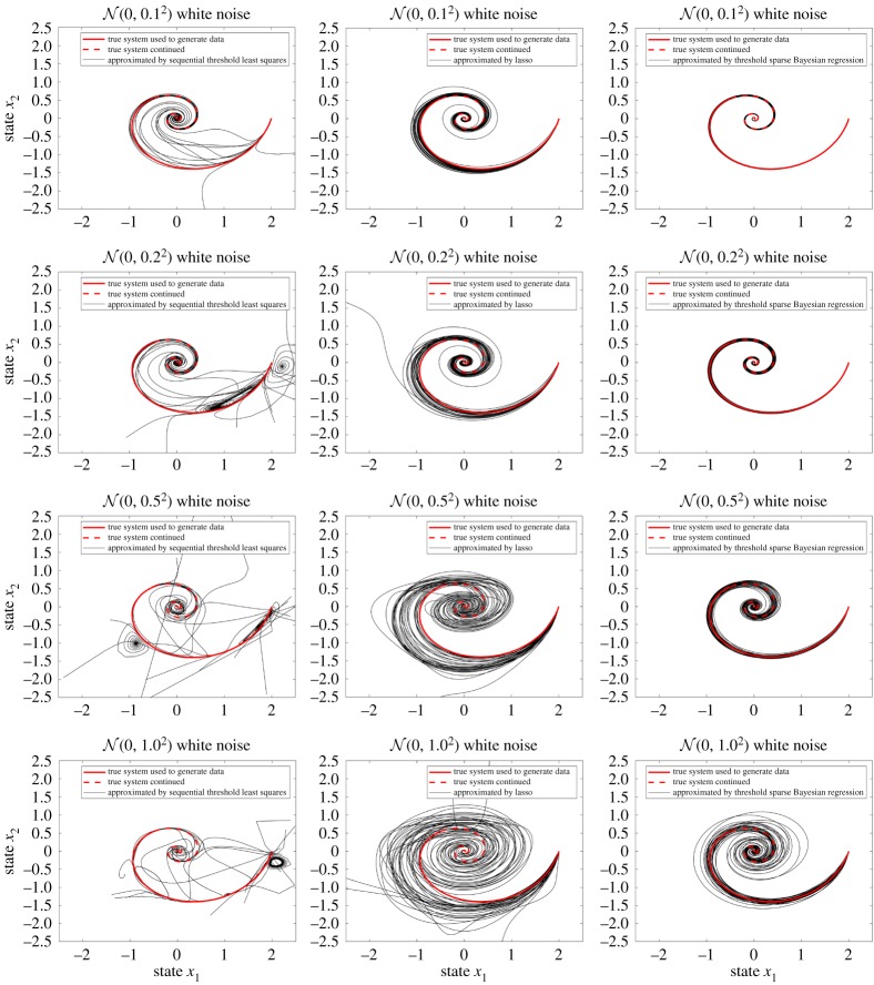
where f is a fixed vector of basis-functions of the form (2.9) whose components are monomials of x₁ and x₂ of up to the fifth degree, and w₁ and w₂ are the weights being solved for. As a comparison, three methods are used individually to discover the dynamical system: sequential threshold least squares (algorithm 2), lasso (algorithm 3) and threshold sparse Bayesian regression (algorithm 1). All the thresholds are set at 0.05. Numerical results are listed in figure 2.

Figure 2.

Thirty simulations of each regression method with different levels of white noise added on dx₁/dt and dx₂/dt. Each regression uses 200 data points. At each level of noise, all regression methods use the same noisy data. (Online version in colour.)

The initial value of the dynamical system is set as (x₁, x₂) = (2, 0). Thirty simulations of each regression method with different levels of white noise added on dx₁/dt and dx₂/dt are illustrated. Randomized simulations provide theoretical justification for the discovery of dynamical systems from random data, which was proved for lasso problems in [8,9,11]. In this example, each regression uses 200 data points. At each level of noise, all regression methods use the same noisy data. As the noise added to the regression methods was random, different solutions are obtained in different runs and yield different curves. Note that discovering a system of equations is equivalent to discovering each equation in the system individually, as long as the data required to calculate the basis-functions are given. As shown in figure 2, threshold sparse Bayesian regression generates better approximated curves to the real solution than sequential threshold least squares and lasso. Furthermore, our method is very robust even for very large noise ($\sim \mathcal{N}(0,{1.0}^2)$).

(b). General automatic discovery and prediction

Consider the Laguerre differential equation:

$$x\frac{{\mathrm{d}}^{2}y}{\mathrm{d}{x}^2}+(1-x)\frac{\mathrm{d}y}{\mathrm{d}x}=0,$$ 4.3

which is (2.3) in §2. We use threshold sparse Bayesian regression with error bar (3.13) to discover this differential equation, and the sets of basis-functions are attempted in sequence starting from ones of lower order. Then we compare the error bars for each result to select a solution. As long as our algorithm gives an error bar that is less than the user-preset value δ = 10⁻⁴, we stop attempting more sets of basis-functions. In this example, basis-functions (2.5)–(2.8) are attempted before the procedure stops. See table 1 for the numerical results with basis-functions (2.8), table 2 with basis-functions (2.5). In total, 20 evenly spaced data are used. This example demonstrates that our method has satisfactory performance even with few data.

Table 1.

Numerical results of discovering the differential equation (4.3) with basis-functions (2.8) using the threshold sparse Bayesian regression with threshold 0.05. Value y in the data is numerically generated by (4.3) in the interval x∈[0.1, 5] with initial value y = y′ = 1. Values y′ and y′′ are calculated using numerical differentiation. In this example, 20 evenly spaced data points (x, y, y′, y′′) in x∈[0.1, 5] are used. The error bar for each result is provided. A smaller error bar means higher posterior confidence and a higher likelihood that the result is correct.

result	1	2	3	4	5	6	7
1		−0.637
x	1
y	−0.079	1
y′		−0.473	1	−0.187	−1.093	0.473	−1.001
y′′				1
x2	0.077				1	−0.426
xy	−0.891				−2.321	1
xy′	1.187		−0.999				1
xy′′			0.999		0.250	−0.107	−1.000
y2	−0.051	−0.427			1.363	−0.595
yy′		0.538
yy′′				−0.715
y′2				0.956
y′y′′				−0.200
y′′2
error bar × 103	10.367	0.108	0.001	6.145	170.614	167.385	0.004

result	8	9	10	11	12	13	14
1
x							0.214
y		−1.013
y′	1.001	1.306	−0.956	0.276	0.753
y′′				−1.255	0.104	−0.487	−7.357
x2
xy		−0.217
xy′	−1.000		−0.090		0.090	0.167
xy′′	1			−0.081			1.913
y2		1					0.363
yy′		−1.283	1		−0.830
yy′′			−0.117	1
y′2			−1.092	−1.163	1	−1.021	−14.290
y′y′′				0.164		1	14.609
y′′2						0.069	1
error bar  × 103	0.004	1.016	0.661	5.317	0.326	8.445	17.589

Table 2.

Numerical results of discovering the differential equation (4.3) with basis-functions (2.5). All other settings are the same as table 1.

result	1	2	3
1	1.195	−0.629	0.625
x	1	−0.362	0.275
y	−2.213	1	−0.994
y′	1.222	−0.727	1
error bar × 103	148.269	37.654	137.530

As shown in table 1, Result 3:

$$y^{\prime }-0.999x{y}^{\prime }+0.999x{y}^{″}=0,$$ 4.4

has the smallest error bar among all of the results, and gives a differential equation similar to an equivalent form of the true differential equation (4.3). Note that Result 3, Result 7 and Result 8 are almost the same. Although some other results with relatively small error bar are not equivalent to the true equation, they might correctly predict its tendency, such as Result 2:

$$-0.637+y-0.473y^{\prime }-0.427y^2+0.538y{y}^{\prime }=0.$$ 4.5

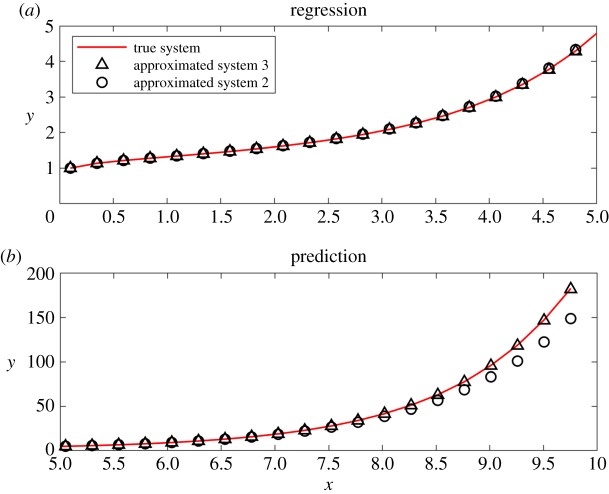
Result 3 has the smallest error bar among all of the results and its numerical solution fits and predicts the true solution well. Result 2 fits the true solution and predicts the tendency correctly, though it has a larger error bar and it is a first-order differential equation, while the true system is of second order. See figure 3 for more details. This example indicates that even if the true system were not discovered, such as in the case where some terms of the true system are not contained in the set of basis-functions, our algorithm could generate an approximated system and provide an accurate regression and prediction of the system's tendency.

Figure 3.

Graphs of approximated systems corresponding to Result 2 and Result 3 in table 1. (a) Numerical solutions and (b) extended solutions as predictions of tendency. (Online version in colour.)

(c). Data-driven discovery of shallow water equations using dimensional analysis and threshold sparse Bayesian regression

Consider the conservative form of shallow water equations:

$$\begin{array}{rl}\frac{\mathrm{\partial }h}{\mathrm{\partial }t}+\frac{\mathrm{\partial }(hu)}{\mathrm{\partial }x}+\frac{\mathrm{\partial }(hv)}{\mathrm{\partial }y}& =0\end{array}$$ 4.6

$$\begin{array}{r}\\ \frac{\mathrm{\partial }(hu)}{\mathrm{\partial }t}+\frac{\mathrm{\partial }(h{u}^2+(1/2)g{h}^2)}{\mathrm{\partial }x}+\frac{\mathrm{\partial }(huv)}{\mathrm{\partial }y}& =0\end{array}$$ 4.7

$$\begin{array}{rl}\text{and}\frac{\mathrm{\partial }(hv)}{\mathrm{\partial }t}+\frac{\mathrm{\partial }(huv)}{\mathrm{\partial }x}+\frac{\mathrm{\partial }(h{v}^2+(1/2)g{h}^2)}{\mathrm{\partial }y}& =0,\end{array}$$ 4.8

where h is the total fluid column height, (u, v) is the fluid's horizontal flow velocity averaged across the vertical column and g is the gravitational acceleration. The first equation can be derived from mass conservation, the last two from momentum conservation. Here, we have made the assumption that the fluid density is a constant.

In this system of partial differential equations, variables h, u, v, ∂h/∂t, ∂u/∂t, ∂v/∂t, ∂h/∂x, ∂u/∂x, ∂v/∂x, ∂h/∂y, ∂u/∂y, ∂v/∂y and constant g ( = 9.8 m s⁻²) are involved. See table 3 for the corresponding dimensions of these variables. The data h, u and v are collected from a numerically generated example, where a water drop falls into a pool with grid size 30 × 30 (figure 4), and then partial derivatives are calculated by central difference formula. As the step size of the numerical differentiation is 1, some errors are introduced to the data. Data means and standard deviations are also provided in table 3 to show the magnitudes of the data. In this example, 1010 data points are used.

Table 3.

Dimensions of the variables, with means and standard deviations of the corresponding data. Here, 1010 data points are used.

variable	dimension	mean	s.d.
h	m	1.051	0.126
u	m s−1	0.001	0.299
v	m s−1	0.002	0.303
∂h/∂t	m s−1	0.000	0.210
∂u/∂t	m s−2	−0.003	0.471
∂v/∂t	m s−2	0.007	0.482
∂h/∂x		0.000	0.044
∂u/∂x	s−1	0.000	0.101
∂v/∂x	s−1	0.001	0.083
∂h/∂y		−0.001	0.046
∂u/∂y	s−1	0.001	0.084
∂v/∂y	s−1	0.000	0.099
g	m s−2	9.8	0

Figure 4.

(a) A water drop falls from height 3 into the spot (14, 15) of a pool with grid size 30 × 30. (b) Water surface of the pool after a period of time. (Online version in colour.)

Now, we use threshold sparse Bayesian regression with threshold 0.1 and the numerically generated data to discover shallow water equations. As the goal is to find the dynamics, regressions for ∂h/∂t, ∂u/∂t and ∂v/∂t are implemented. As ∂h/∂t has the dimension of speed (m s⁻¹), we assume that it is a linear combination of variables of the same dimension. These variables can be constructed as products of h, u, v, their first-order derivatives, and the constant g; namely, h(∂u/∂x), h(∂v/∂x), h(∂u/∂y), h(∂v/∂y), u, u(∂h/∂x), u(∂h/∂y), v, v(∂h/∂x), v(∂h/∂y), (∂h/∂t)(∂h/∂x), (∂h/∂t)(∂h/∂y). Using the data with threshold sparse Bayesian regression, we have the following result:

$$\frac{\mathrm{\partial }h}{\mathrm{\partial }t}=-1.010(\pm 0.002)h\frac{\mathrm{\partial }u}{\mathrm{\partial }x}-1.004(\pm 0.002)h\frac{\mathrm{\partial }v}{\mathrm{\partial }y}-0.901(\pm 0.012)u\frac{\mathrm{\partial }h}{\mathrm{\partial }x}-0.932(\pm 0.012)v\frac{\mathrm{\partial }h}{\mathrm{\partial }y},$$ 4.9

where the numbers in front of each term read as ‘mean ( ± s.d.)’ of the corresponding weights. The magnitudes of the data u(∂h/∂x) and v(∂h/∂y) are small compared to ∂h/∂t, h(∂u/∂x) and h(∂v/∂y) (table 3), which means u(∂h/∂x) and v(∂h/∂y) are tiny terms in the differential equations and easily covered by noise. Hence, the resulting weights of u(∂h/∂x) and v(∂h/∂y) are not as accurate as that of h(∂u/∂x) and h(∂v/∂y).

As u(∂u/∂x), u(∂v/∂x), u(∂u/∂y), u(∂v/∂y), v(∂u/∂x), v(∂v/∂x), v(∂u/∂y), v(∂v/∂y), (∂h/∂t)(∂u/∂x), (∂h/∂t)(∂v/∂x), (∂h/∂t)(∂u/∂y), (∂h/∂t)(∂v/∂y), ∂u/∂t, ∂v/∂t, g(∂h/∂x), g(∂h/∂y) have the dimension of acceleration (m s⁻²), using the same procedure as above, our algorithm generates the following result:

$$\frac{\mathrm{\partial }u}{\mathrm{\partial }t}=-0.899(\pm 0.010)u\frac{\mathrm{\partial }u}{\mathrm{\partial }x}-0.940(\pm 0.012)v\frac{\mathrm{\partial }u}{\mathrm{\partial }y}-1.008(\pm 0.001)g\frac{\mathrm{\partial }h}{\mathrm{\partial }x}$$ 4.10

and

$$\frac{\mathrm{\partial }v}{\mathrm{\partial }t}=-0.953(\pm 0.013)u\frac{\mathrm{\partial }v}{\mathrm{\partial }x}-0.886(\pm 0.010)v\frac{\mathrm{\partial }v}{\mathrm{\partial }y}-1.011(\pm 0.001)g\frac{\mathrm{\partial }h}{\mathrm{\partial }y}.$$ 4.11

Again, the resulting weights of u(∂u/∂x), v(∂u/∂y), u(∂v/∂x) and v(∂v/∂y) have relatively large errors due to small magnitudes of the corresponding data, and fundamentally, due to the intrinsic properties of the investigated differential equations.

System of equations (4.9)–(4.11) is a good approximation to the following system of equations

$$\begin{array}{rl}\frac{\mathrm{\partial }h}{\mathrm{\partial }t}+h\frac{\mathrm{\partial }u}{\mathrm{\partial }x}+h\frac{\mathrm{\partial }v}{\mathrm{\partial }y}+u\frac{\mathrm{\partial }h}{\mathrm{\partial }x}+v\frac{\mathrm{\partial }h}{\mathrm{\partial }y}& =0,\end{array}$$ 4.12

$$\begin{array}{r}\\ \frac{\mathrm{\partial }u}{\mathrm{\partial }t}+u\frac{\mathrm{\partial }u}{\mathrm{\partial }x}+v\frac{\mathrm{\partial }u}{\mathrm{\partial }y}+g\frac{\mathrm{\partial }h}{\mathrm{\partial }x}& =0\end{array}$$ 4.13

$$\begin{array}{rl}\text{and}\frac{\mathrm{\partial }v}{\mathrm{\partial }t}+u\frac{\mathrm{\partial }v}{\mathrm{\partial }x}+v\frac{\mathrm{\partial }v}{\mathrm{\partial }y}+g\frac{\mathrm{\partial }h}{\mathrm{\partial }y}& =0,\end{array}$$ 4.14

which is equivalent to the system of equations (4.6)–(4.8). This example indicates that our algorithm may discover an equivalent form of the true system.

(d). Data-driven discovery of Navier–Stokes equations using dimensional analysis and threshold sparse Bayesian regression

Consider the following two-dimensional incompressible Navier–Stokes equations:

$$\frac{\mathrm{\partial }\mathit{u}}{\mathrm{\partial }t}+[\mathit{u}\cdot \mathrm{\nabla }]\mathit{u}-\nu \mathrm{△}\mathit{u}=-\mathrm{\nabla }\left(\frac{p}{\rho }\right),$$ 4.15

where u is the flow velocity, ν is the kinematic viscosity, p is the pressure and ρ is the density. Letting u = (u₁, u₂), where u₁ is the flow velocity in x direction and u₂ is the flow velocity in y direction, we have:

$$\frac{\mathrm{\partial }{u}_1}{\mathrm{\partial }t}=-u_1\frac{\mathrm{\partial }{u}_1}{\mathrm{\partial }x}-v\frac{\mathrm{\partial }{u}_1}{\mathrm{\partial }y}+\nu \frac{{\mathrm{\partial }}^2{u}_1}{\mathrm{\partial }{x}^2}+\nu \frac{{\mathrm{\partial }}^2{u}_1}{\mathrm{\partial }{y}^2}-\frac{\mathrm{\partial }(p/\rho )}{\mathrm{\partial }x}$$ 4.16

and

$$\frac{\mathrm{\partial }{u}_2}{\mathrm{\partial }t}=-u\frac{\mathrm{\partial }{u}_2}{\mathrm{\partial }x}-v\frac{\mathrm{\partial }{u}_2}{\mathrm{\partial }y}+\nu \frac{{\mathrm{\partial }}^2{u}_2}{\mathrm{\partial }{x}^2}+\nu \frac{{\mathrm{\partial }}^2{u}_2}{\mathrm{\partial }{y}^2}-\frac{\mathrm{\partial }(p/\rho )}{\mathrm{\partial }y}.$$ 4.17

In this system of equations, variables u₁, u₂, ∂u₁/∂t, ∂u₂/∂t, ∂u₁/∂x, ∂u₂/∂x, ∂u₁/∂y, ∂u₂/∂y, ∂²u₁/∂x², ∂²u₂/∂x², ∂²u₁/∂y², ∂²u₂/∂y², p/ρ, ∂(p/ρ)/∂x, ∂(p/ρ)/∂y and ν are involved. See table 4 for the corresponding (u₁, u₂) dimensions of these variables. We set ρ, ν as constants and collect data u₁, u₂, p from a numerically generated example (figure 5) and then compute partial derivatives using the central-difference formula.

Table 4.

Variables and their dimensions.

variable	u1	u2	∂u1/∂t	∂u2/∂t	∂u1/∂x	∂u2/∂x
dimension	m s−1	m s−1	m s−2	m s−2	s−1	s−1

variable	∂u1/∂y	∂u2/∂y	∂2u1/∂x2	∂2u2/∂x2	∂2u1/∂y2	∂2u2/∂y2
dimension	s−1	s−1	(m · s)−1	(m · s)−1	(m · s)−1	(m · s)−1

variable	p/ρ	∂(p/ρ)/∂x	∂(p/ρ)/∂y	ν
dimension	m2 s−2	m s−2	m s−2	m2 s−1

Figure 5.

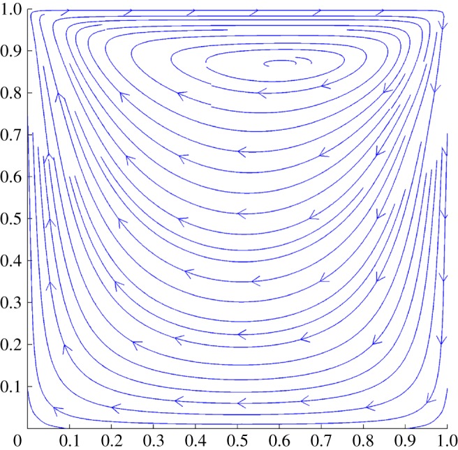
Incompressible Navier–Stokes equations. (Online version in colour.)

Now we use threshold sparse Bayesian regression with threshold 0.1 and the numerically generated data to discover Navier–Stokes equations. As ∂u₁/∂t and ∂u₂/∂t have the dimension of acceleration (m s⁻²), we assume that they are linear combinations of variables of the same dimension. Similar to the example for shallow water equations discussed above, the basis-functions can be constructed as u₁(∂u₁/∂x), u₁(∂u₁/∂y), u₁(∂u₂/∂x), u₁(∂u₂/∂y), u₂(∂u₁/∂x), u₂(∂u₁/∂y), u₂(∂u₂/∂x), u₂(∂u₂/∂y), ν(∂²u₁/∂x²), ν(∂²u₁/∂y²), ν(∂²u₂/∂x²), ν(∂²u₂/∂y²), ∂(p/ρ)/∂x, ∂(p/ρ)/∂y. In this example, 202 data points are used. Using the data with threshold sparse Bayesian regression, our algorithm generates the following result:

$$\begin{array}{rl}\frac{\mathrm{\partial }{u}_1}{\mathrm{\partial }t}& =-0.982(\pm 0.002)u_1\frac{\mathrm{\partial }{u}_1}{\mathrm{\partial }x}-0.984(\pm 0.001)u_2\frac{\mathrm{\partial }{u}_1}{\mathrm{\partial }y}+0.972(\pm 0.002)\nu \frac{{\mathrm{\partial }}^2{u}_1}{\mathrm{\partial }{x}^2}\\ & +0.999(\pm 0.001)\nu \frac{{\mathrm{\partial }}^2{u}_1}{\mathrm{\partial }{y}^2}-0.998(\pm 0.001)\frac{\mathrm{\partial }(p/\rho )}{\mathrm{\partial }x}\end{array}$$ 4.18

and

$$\begin{array}{rl}\frac{\mathrm{\partial }{u}_2}{\mathrm{\partial }t}& =-0.990(\pm 0.001)u_1\frac{\mathrm{\partial }{u}_2}{\mathrm{\partial }x}-1.008(\pm 0.001)u_2\frac{\mathrm{\partial }{u}_2}{\mathrm{\partial }y}+1.005(\pm 0.001)\nu \frac{{\mathrm{\partial }}^2{u}_2}{\mathrm{\partial }{x}^2}\\ & +0.987(\pm 0.001)\nu \frac{{\mathrm{\partial }}^2{u}_2}{\mathrm{\partial }{y}^2}-1.002(\pm 0.001)\frac{\mathrm{\partial }(p/\rho )}{\mathrm{\partial }y},\end{array}$$ 4.19

with error bars 1.093 × 10⁻⁵ and 6.415 × 10⁻⁶, respectively, where the numbers in front of each term read as ‘mean ( ± s.d.)’ of the corresponding weights. Next, we try to discover more identities in this system with the procedure similar to what we did for (4.3). Here, all the terms of dimension (m s⁻²) except for ∂u₁/∂t and ∂u₂/∂t are chosen as basis-functions. See table 5 for the numerical results. The identity ∂u₁/∂x + ∂u₂/∂y = 0 is successfully discovered.

Table 5.

Discovery of identities in Navier–Stokes equations using threshold sparse Bayesian regression with threshold 0.1. Here, 202 data are used. Result 1, Result 4, Result 5, Result 8 have the smallest error bars, and they are equivalent to the identity ∂u₁/∂x + ∂u₂/∂y = 0.

result	1	2	3	4	5	6	7
u1∂u1/∂x	1			1.000		−0.396
u1∂u1/∂y		1
u1∂u2/∂x		2.271	1			−0.349	−0.231
u1∂u2/∂y	1.000	−0.909		1		0.993
u2∂u1/∂x		1.746			1
u2∂u1/∂y		−0.608				1	−0.204
u2∂u2/∂x		4.997	0.154			−1.223	1
u2∂u2/∂y					1.000	−0.575
ν∂2u1/∂x2		−3.389	−0.632			0.676	−0.534
ν∂2u1/∂y2		−1.366
ν∂2u2/∂x2		2.455				−0.613	0.657
ν∂2u2/∂y2		−7.156	−0.351			2.774	−1.111
∂(p/ρ)/∂x			−0.100			0.209
∂(p/ρ)/∂y		−1.008					−0.294
error bar  × 103	0.000	1110.362	183.139	0.000	0.000	3139.186	127.743

result	8	9	10	11	12	13	14
u1∂u1/∂x			−1.179
u1∂u1/∂y			−0.220
u1∂u2/∂x		−0.388				−1.290	0.721
u1∂u2/∂y							−0.640
u2∂u1/∂x	1.000		−0.478
u2∂u1/∂y		0.119		−0.193	0.203	0.533
u2∂u2/∂x		−0.387	−2.059	0.770	−0.468	−0.867	−1.043
u2∂u2/∂y	1						0.581
ν∂2u1/∂x2		1	2.436	−0.745	0.232	−0.441	0.489
ν∂2u1/∂y2			1			−0.463
ν∂2u2/∂x2		−0.317	−1.002	1	−0.128	−0.274	−1.515
ν∂2u2/∂y2		0.463	3.272	−0.521	1	1.233	−0.116
∂(p/ρ)/∂x			−0.796			1
∂(p/ρ)/∂y		0.128	0.370	−0.473			1
error bar × 103	0.000	189.638	332.790	88.404	48.410	358.041	1081.667

(e). Threshold sparse Bayesian regression for prediction

Consider the function from $\mathbb{R}$ to $\mathbb{R}$:

$$f(x)=1+x+10{\text{e}}^{-x},$$ 4.20

which satisfies

$$f^{\prime }=2+x-f.$$ 4.21

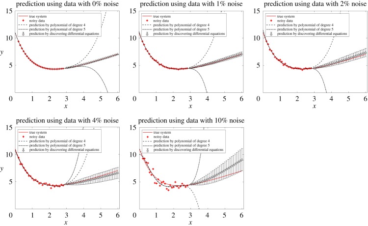
Given its values on the interval [0, 3], we try to predict its values on [3, 6]. We will compare polynomial regressions with the method of discovering differential equations. Different levels of noise are analysed. Although the method of discovering differential equations uses less data and introduces more error when calculating numerical derivatives, it has much better performance in prediction than polynomial regressions (figure 6).

Figure 6.

Comparison of polynomial regressions with the method of discovering differential equations in the prediction of (4.20). Different levels of noise are studied. In this example, 31 equally spaced data points with step size 0.1 are collected on [0, 3]. Polynomial regressions use all of the 31 data points, but for discovering differential equations, we calculate the derivatives of the middle 27 data points using central difference formula. Then the other four data points are discarded and only 27 data points are used in our algorithm. The prediction by discovering differential equations at each x reads as ‘mean ( ± s.d.)’. Although the method of discovering differential equations uses less data points and introduces more error when calculating numerical derivatives, it has much better performance in prediction than polynomial regressions. (Online version in colour.)

Root mean square prediction error by polynomial regression and the method of discovering differential equations, as well as the discovered differential equation are listed in table 6, with no noise, 1% noise, 2% noise, 4% noise, and 10% noise, respectively. At all levels of noise, the method of discovering differential equations performs better than polynomial regressions.

Table 6.

Root mean square prediction error by polynomial regression and the method of discovering differential equations, as well as the discovered differential equation, at each noise level. The predictions by our algorithm have much less error than the predictions by polynomial regressions.

noise (%)	root mean square prediction error by polynomial regression of degree 4	root mean square prediction error by discovering differential equations
0	7.3052	0.0001
1	14.4525	0.0479
2	21.6053	0.2083
4	19.7245	0.2369
10	73.0118	1.0310
noise (%)	discovered differential equation
0	dy/dx = 2.000( ± 0.005) + 1.000( ± 0.001)x − 1.000( ± 0.001)y
1	dy/dx = 1.997( ± 0.221) + 1.015( ± 0.051)x − 1.000( ± 0.027)y
2	dy/dx = 1.772( ± 0.430) + 1.076( ± 0.099)x − 0.972( ± 0.053)y
4	dy/dx = 2.625( ± 0.649) + 0.897( ± 0.152)x − 1.097( ± 0.081)y
10	dy/dx =  − 0.921( ± 0.774) + 1.426( ± 0.220)x − 0.622( ± 0.096)y

In the discovered differential equations of our algorithm, the weight of each term is of normal distribution, and the numbers in front of each term read as ‘mean ( ± s.d.)’ of the corresponding weights (table 6). In total, 10 000 Monte Carlo samples of the weights are performed to produce 10 000 curves of numerical solutions, or 10 000 predictive values at each x. Then the means and standard deviations are calculated for each x to quantify the uncertainty (figure 6).

Now consider a second example, the function from $\mathbb{R}$ to $\mathbb{R}$:

$$f(x)=1+x+2\sin (x),$$ 4.22

which satisfies

$$f^{\prime }=1+2\cos (x).$$ 4.23

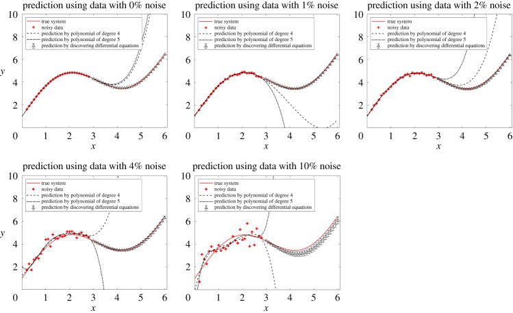
With all settings the same as the first example, we have our results in figure 7 and table 7. Again, the method of discovering differential equations has much better performance in prediction than polynomial regressions. These two examples show how our algorithm exploits the characteristics of the models in terms of differential equations and that our algorithm is applicable to models where polynomial regressions fail.

Figure 7.

Comparison of polynomial regressions with the method of discovering differential equations in the prediction of (4.22). All settings are the same as those in figure 6. The method of discovering differential equations has much better performance in prediction than polynomial regressions. (Online version in colour.)

Table 7.

Root mean square prediction error by polynomial regression and the method of discovering differential equations, as well as the discovered differential equation, at each noise level. The predictions by our algorithm have much less error than the predictions by polynomial regressions.

noise (%)	root mean square prediction error by polynomial regression of degree 4	root mean square prediction error by discovering differential equations
0	4.5316	0.0000
1	3.3486	0.0277
2	3.8464	0.0583
4	33.1033	0.0561
10	99.8210	0.3243
noise (%)	discovered differential equation
0	dy/dx = 1.000( ± 0.000) + 2.000( ± 0.000)cos(x)
1	dy/dx = 0.997( ± 0.008) + 2.027( ± 0.013)cos(x)
2	dy/dx = 0.984( ± 0.015) + 2.039( ± 0.023)cos(x)
4	dy/dx = 0.954( ± 0.040) + 1.964( ± 0.061)cos(x)
10	dy/dx = 0.908( ± 0.100) + 2.208( ± 0.155)cos(x)

(f). Choice of the threshold in threshold sparse Bayesian regression

In this section, we will investigate how the threshold impacts the accuracy of the result and how to choose the threshold. Consider the same dynamical system in example 4a:

$$\begin{array}{rl}\frac{\mathrm{d}{x}_1}{\mathrm{d}t}& =-0.5x_1+2x_2\\ \mathrm{and}\frac{\mathrm{d}{x}_2}{\mathrm{d}t}& =-2x_1-0.5x_2.\end{array}\}$$ 4.24

We try to discover the first differential equation in the system (4.24) using our algorithm, at different levels of threshold.

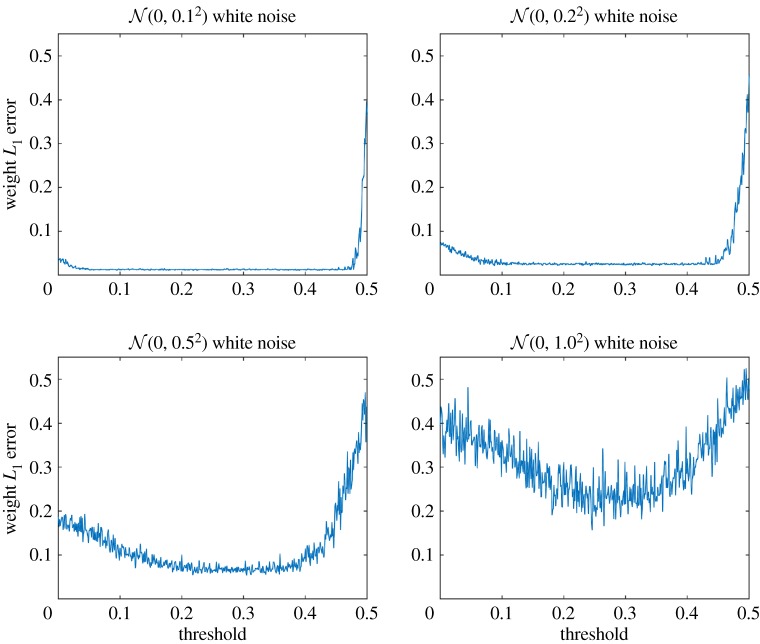
The initial value of the dynamical system is set as (x₁, x₂) = (2, 0). One hundred simulations at each level of threshold per level of white noise added on dx₁/dt are performed. Each simulation uses 200 data points. As the noise is random, different solutions are obtained in different simulations and yield different results. For each result, we calculate the L₁ error between the discovered weight-vector and the true weight-vector. Then, the L₁ errors are averaged among the same level of threshold. See figure 8 for the weight L₁ error by threshold.

Figure 8.

Weight L₁ error by threshold at each level of white noise. One hundred simulations at each level of threshold per level of white noise added on dx₁/dt are performed. Each simulation uses 200 data points. (Online version in colour.)

As shown in figure 8, weight L₁ error is large when the threshold approaches 0 or 0.5. Weight L₁ error is large at 0 because the algorithm is unable to clean up possible disturbances present in the weight-vector. Note that one of the true weights in the first differential equation in the system (4.24) is −0.5. When the threshold is around 0.5, this term may be falsely eliminated, which causes a huge error jump. When the threshold is between 0.15 and 0.4, our algorithm generates the best results. This example indicates that the best choices of threshold should be moderately greater than 0 but not too large.

5. Conclusion

We have introduced a new data-driven approach, the threshold sparse Bayesian regression algorithm, to find physical laws by discovering differential equations from noisy data. The proposed method is a different approach than the regression-like method called symbolic regression in [1]. Symbolic regression distills physical laws from data directly, without involving differential equations. Similar approaches as the proposed method were studied in [5–22,37]. In this work, a hierarchical Bayesian framework has been constructed to provide error bars that quantify the uncertainties of the discovered physical laws. The key idea is to select candidate terms for the underlying equations using dimensional analysis, and to approximate the weights of the terms with error bars using our new algorithm, the threshold sparse Bayesian regression algorithm, which employs Bayesian inference to tune the hyperparameters automatically.

Our approach is effective, robust and able to quantify uncertainties by providing an error bar for each discovered candidate equation. The effectiveness of our algorithm is demonstrated through a collection of classical ordinary differential equations and partial differential equations. Within this framework, we have provided six numerical examples in §4 to examine the performance of the proposed method. Example 4a has compared the proposed method with other sparse regression methods, the sequential threshold least-squares algorithm and the lasso algorithm. It demonstrates that the proposed method has better performance and robustness than the other methods. Example 4b has applied the general discovery pattern introduced earlier in this paper and tested the constructed error bars. The numerical results demonstrate that the proposed pattern is practical. Examples 4c,d have combined dimensional analysis with the proposed method to discover shallow water equations and Navier–Stokes equations, and have demonstrated the practical usage of the proposed algorithm. Example 4e has illustrated more accurate and robust predictions of the dynamics using the proposed algorithm, as compared to the predictions of polynomial regressions. Example 4f has discussed how to choose the threshold in the proposed algorithm.

Ethics

This work did not involve any active collection of human data, but only computer simulations.

Data accessibility

All data used in this manuscript are publicly available on http://www.math.purdue.edu/∼lin491/data/LE

Author's contributions

S.Z. conceived the mathematical models, implemented the methods, designed the numerical experiments, interpreted the results and wrote the paper. G.L. supported this study and reviewed the final manuscript. All the authors gave their final approval for publication.

Competing interests

We declare we have no competing interests.

Funding

We gratefully acknowledge the support from National Science Foundation (DMS-1555072, DMS-1736364 and DMS-1821233).

References

- 1.Schmidt M, Lipson H. 2009. Distilling free-form natural laws from experimental data. Science 324, 81–85. ( 10.1126/science.1165893) [DOI] [PubMed] [Google Scholar]
- 2.Anderson PW. 1972. More is different. Science 177, 393–396. ( 10.1126/science.177.4047.393) [DOI] [PubMed] [Google Scholar]
- 3.Hanc J, Tuleja S, Hancova M. 2004. Symmetries and conservation laws: consequences of Noether's theorem. Am. J. Phys. 72, 428–435. ( 10.1119/1.1591764) [DOI] [Google Scholar]
- 4.Holton GJ, Brush SG. 2001. Physics, the human adventure: from Copernicus to Einstein and beyond. New Brunswick, NJ: Rutgers University Press. [Google Scholar]
- 5.Brunton SL, Proctor JL, Kutz JN. 2016. Discovering governing equations from data by sparse identification of nonlinear dynamical systems. Proc. Natl Acad. Sci. USA 113, 3932–3937. ( 10.1073/pnas.1517384113) [DOI] [PMC free article] [PubMed] [Google Scholar]
- 6.Schaeffer H. 2017. Learning partial differential equations via data discovery and sparse optimization. Proc. R. Soc. A 473, 20160446 ( 10.1098/rspa.2016.0446) [DOI] [PMC free article] [PubMed] [Google Scholar]
- 7.Schaeffer H, McCalla SG. 2017. Sparse model selection via integral terms. Phys. Rev. E 96, 023302 ( 10.1103/PhysRevE.96.023302) [DOI] [PubMed] [Google Scholar]
- 8.Schaeffer H, Tran G, Ward R. 2017 Extracting sparse high-dimensional dynamics from limited data. (http://arxiv.org/abs/1707.08528. )
- 9.Schaeffer H, Tran G, Ward R, Zhang L. 2018 Extracting structured dynamical systems using sparse optimization with very few samples. (http://arxiv.org/abs/1805.04158. )
- 10.Rudy SH, Brunton SL, Proctor JL, Kutz JN. 2017. Data-driven discovery of partial differential equations. Sci. Adv. 3, e1602614 ( 10.1126/sciadv.1602614) [DOI] [PMC free article] [PubMed] [Google Scholar]
- 11.Tran G, Ward R. 2017. Exact recovery of chaotic systems from highly corrupted data. Multiscale Model. Simul. 15, 1108–1129. ( 10.1137/16M1086637) [DOI] [Google Scholar]
- 12.Mangan NM, Kutz JN, Brunton SL, Proctor JL. 2017. Model selection for dynamical systems via sparse regression and information criteria. Proc. R. Soc. A 473, 20170009 ( 10.1098/rspa.2017.0009) [DOI] [PMC free article] [PubMed] [Google Scholar]
- 13.Kaiser E, Kutz JN, Brunton SL. 2017 Sparse identification of nonlinear dynamics for model predictive control in the low-data limit. (http://arxiv.org/abs/1711.05501. )
- 14.Loiseau J-C, Brunton SL. 2018. Constrained sparse Galerkin regression. J. Fluid Mech. 838, 42–67. ( 10.1017/jfm.2017.823) [DOI] [Google Scholar]
- 15.Quade M, Abel M, Kutz JN, Brunton SL. 2018 doi: 10.1063/1.5027470. Sparse identification of nonlinear dynamics for rapid model recovery. (http://arxiv.org/abs/1803.00894) [DOI] [PubMed]
- 16.Zhang L, Schaeffer H. 2018 On the convergence of the sindy algorithm. (http://arxiv.org/abs/1805.06445)
- 17.Mangan NM, Brunton SL, Proctor JL, Kutz JN. 2016. Inferring biological networks by sparse identification of nonlinear dynamics. IEEE Trans. Mol. Biol. Multi-Scale Commun. 2, 52–63. ( 10.1109/TMBMC.2016.2633265) [DOI] [Google Scholar]
- 18.Daniels BC, Nemenman I. 2015. Automated adaptive inference of phenomenological dynamical models. Nat. Commun. 6, 8133 ( 10.1038/ncomms9133) [DOI] [PMC free article] [PubMed] [Google Scholar]
- 19.Daniels BC, Nemenman I. 2015. Efficient inference of parsimonious phenomenological models of cellular dynamics using s-systems and alternating regression. PLoS ONE 10, e0119821 ( 10.1371/journal.pone.0119821) [DOI] [PMC free article] [PubMed] [Google Scholar]
- 20.Dam M, Brøns M, Juul Rasmussen J, Naulin V, Hesthaven JS. 2017. Sparse identification of a predator-prey system from simulation data of a convection model. Phys. Plasmas 24, 022310 ( 10.1063/1.4977057) [DOI] [Google Scholar]
- 21.Boninsegna L, Nüske F, Clementi C. 2017 Sparse learning of stochastic dynamic equations. (http://arxiv.org/abs/1712.02432. )
- 22.Sorokina M, Sygletos S, Turitsyn S. 2016. Sparse identification for nonlinear optical communication systems: Sino method. Opt. Express 24, 30433 ( 10.1364/OE.24.030433) [DOI] [PubMed] [Google Scholar]
- 23.Tibshirani R. 1996. Regression shrinkage and selection via the lasso. J. R. Stat. Soc. B (Methodological) 58, 267–288. [Google Scholar]
- 24.Tipping ME. 2001. Sparse Bayesian learning and the relevance vector machine. J. Mach. Learn. Res. 1, 211–244. ( 10.1162/15324430152748236) [DOI] [Google Scholar]
- 25.Tipping ME. 2004. Bayesian inference: an introduction to principles and practice in machine learning. Lecture Notes in Computer Science, vol. 3176, pp. 41–62. Berlin, Germany: Springer. [Google Scholar]
- 26.Ji S, Xue Y, Carin L. 2008. Bayesian compressive sensing. IEEE Trans. Signal Process. 56, 2346–2356. ( 10.1109/TSP.2007.914345) [DOI] [Google Scholar]
- 27.Ji S, Dunson D, Carin L. 2009. Multitask compressive sensing. IEEE Trans. Signal Process. 57, 92–106. ( 10.1109/tsp.2008.2005866) [DOI] [PMC free article] [PubMed] [Google Scholar]
- 28.Candes EJ, Romberg JK, Tao T. 2006. Stable signal recovery from incomplete and inaccurate measurements. Commun. Pure Appl. Math. 59, 1207–1223. ( 10.1002/cpa.20124) [DOI] [Google Scholar]
- 29.Candes E, Romberg J. 2007. Sparsity and incoherence in compressive sampling. Inverse. Probl. 23, 969–985. ( 10.1088/0266-5611/23/3/008) [DOI] [Google Scholar]
- 30.Baraniuk RG. 2007. Compressive sensing [lecture notes]. IEEE Signal. Process. Mag. 24, 118–121. ( 10.1109/msp.2007.4286571) [DOI] [Google Scholar]
- 31.Elad M, Aharon M. 2006. Image denoising via sparse and redundant representations over learned dictionaries. IEEE Trans. Image. Process. 15, 3736–3745. ( 10.1109/tip.2006.881969) [DOI] [PubMed] [Google Scholar]
- 32.Mairal J, Bach F, Ponce J, Sapiro G. 2009. Online dictionary learning for sparse coding. In Proc. of the 26th Annual International Conference on Machine Learning, Montreal, Canada, 14–18 June, pp. 689–696. New York, NY: ACM.
- 33.Qu Q, Sun J, Wright J. 2014. Finding a sparse vector in a subspace: linear sparsity using alternating directions. IEEE Trans. Information Theory 62, 5855–5880. ( 10.1109/TIT.2016.2601599) [DOI] [Google Scholar]
- 34.Cengel YA, Cimbala JM, Fluid mechanics fundamentals and applications, 185201 International Edition. New York, NY: McGraw Hill Publications. [Google Scholar]
- 35.Berger JO. 2013. Statistical decision theory and Bayesian analysis. Berlin, Germany: Springer Science & Business Media. [Google Scholar]
- 36.Tipping ME, Faul AC. 2003. Fast marginal likelihood maximisation for sparse Bayesian models. In Proc. of the Ninth Int. Workshop on Artificial Intelligence and Statistics, AISTAT 2003, Key West, FL: 3–6 January. New Jersey: Society for Artificial Intelligence and Statistics.
- 37.Bongard J, Lipson H. 2007. Automated reverse engineering of nonlinear dynamical systems. Proc. Natl Acad. Sci. USA 104, 9943–9948. ( 10.1073/pnas.0609476104) [DOI] [PMC free article] [PubMed] [Google Scholar]
Associated Data
This section collects any data citations, data availability statements, or supplementary materials included in this article.
Data Availability Statement