Radio-pathomic Maps of Epithelium and Lumen Density Predict the Location of High-Grade Prostate Cancer

Abstract

Purpose:

This study aims to combine multiparametric magnetic resonance imaging (MRI) and digitized pathology with machine learning to generate predictive maps of histologic features for prostate cancer localization.

Methods and Materials:

Thirty-nine patients underwent MRI prior to prostatectomy. After surgery, tissue was sliced according to MRI orientation using patient-specific 3-dimensionally printed slicing jigs. Whole-mount sections were annotated by our pathologist and digitally contoured to differentiate the lumen and epithelium. Slides were co-registered to the T2-weighted MRI scan. A learning curve was generated to determine the number of patients required for a stable machine-learning model. Patients were randomly stratified into 2 training sets and 1 test set. Two partial least-squares regression models were trained, each capable of predicting lumen and epithelium density. Predicted density values were calculated for each patient in the test dataset, mapped into the MRI space, and compared between regions confirmed as high-grade prostate cancer.

Results:

The learning-curve analysis showed that a stable fit was achieved with data from 10 patients. Maps indicated that regions of increased epithelium and decreased lumen density, generated from each independent model, corresponded with pathologist-annotated regions of high-grade cancer.

Conclusions:

We present a radio-pathomic approach to mapping prostate cancer. We find that the maps are useful for highlighting high-grade tumors. This technique may be relevant for dose-painting strategies in prostate radiation therapy. © 2018 The Author(s). Published by Elsevier Inc. This is an open access article under the CC BY-NC-ND license (http://creativecommons.org/licenses/by-nc-nd/4.0/).

Summary

This study aims to combine whole-mount prostate pathology with multiparametric magnetic resonance imaging from 39 patients to generate predictive maps of epithelium and lumen density in magnetic resonance imaging space. We show that the new image contrasts generated stratify high-grade tumors from low-grade tumors and healthy tissue. Future studies will explore targeted radiation therapy and clinical disease staging using the radio-pathomic mapping technique.

Introduction

Prostate cancer will be diagnosed in 1 in 7 men, although not all cases are clinically significant (1). Gleason grade 3 (G3) cancers often never progress to metastatic cancer, while Gleason grade 4 (G4) and grade 5 (G5) cancers are more likely to progress and cause death (2). Differentiation of indolent from aggressive disease is therefore a major focus of ongoing radiologic studies.

Multiparametric (MP) magnetic resonance imaging (MRI) including diffusion and perfusion imaging has recently shown promise in improving the diagnostic accuracy in high-grade prostate cancer (3, 4). Ongoing standardization efforts have also improved the consistency of radiologist reports (5, 6). Studies have shown that MP-MRI is useful for biopsy guidance (7) and potentially selective radiation therapy boost strategies (8). Noninvasive imaging is therefore becoming standard for staging and localizing prostate cancer.

Radiomics describes the field of study in which images are treated as mineable databases to solve classification problems (9, 10). Image features, which can be a statistical expression of pixel neighborhood or tumor morphometry, as well as clinical variables (9, 11, 12), are used as inputs to classification algorithms. Models can then be used to detect and characterize a clinically relevant outcome (12–15).

“Rad-path” correlation is the integration of radiology and pathology, in which diagnostic information from tissue is aligned with medical imaging. Whole-mount tissue alignment has allowed the measurement of tissue heterogeneity across large regions that include many voxels and various degrees of cancer aggressiveness (16–18).

This study presents a technique, radio-pathomic mapping, that combines whole-mount prostate rad-path with machine learning to generate predictive maps of pathologic features based on noninvasive imaging alone. Two machine-learning models were generated from separate training datasets and subsequently applied to a naive test dataset. We hypothesized that radio-pathomic maps of epithelium and lumen density would highlight regions of high-grade prostate cancer, which has direct implications for the radiation oncology community.

Methods and Materials

Patient population

We prospectively recruited 39 patients undergoing MPMRI prior to prostatectomy for this institutional review board-approved study. Written consent was obtained from all patients, who ranged in age from 45 to 72 years (mean, 60 years). The average prostate-specific antigen score measured prior to surgery was 8.2 ng/mL, with a range of 2.8 to 27.5 ng/mL. Eligible patients were identified and recruited consecutively. The distribution of tumor burden in the cohort is shown in Table E1 (available online at www.redjournal.org).

Imaging

MP-MRI was acquired on a 3-T MRI scanner (General Electric, Waukesha, WI) using an endorectal coil. MP-MRI included field-of-view optimized and constrained undistorted single shot (FOCUS) diffusion weighted imaging with 10 b values (0, 10, 25, 50, 80, 100, 200, 500, 1000, and 2000), dynamic contrast-enhanced imaging, and T2-weighted imaging (19). A summary of imaging parameters is shown in Table E2 (available online at www.redjournal.org).

MRI preprocessing

To correct for intersubject intensity variation, T2-weighted images were intensity normalized using previously published techniques (12). Apparent diffusion coefficient (ADC) maps were calculated from different combinations of b values. The image with b Z 0 was aligned with the T2 image using FMRIB’s Linear Image Registration Tool (Functional Magnetic Resonance Imaging of the Brain Library, Oxford, UK), and all resulting diffusion maps were transformed into the T2 space using the calculated transformation matrix (20). Alignment was verified and manually corrected if misregistration occurred by use of the tkregister tool from FreeSurfer (surfer.nmr.mgh.harvard.edu). Contrast uptake was calculated from the dynamic contrast-enhanced imaging.

Surgery

Robotic prostatectomy was performed using the da Vinci robotic system (Intuitive Surgical, Sunnyvale, CA). All surgical procedures were performed by a single fellowship-trained surgeon (KJ) using a robotic surgical technique (21, 22). Surgical specimens were extracted en bloc and fixed in formalin.

Tissue sectioning

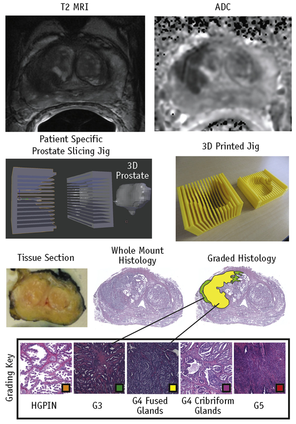
Prostate samples were inked and sectioned using patient-specific tissue-slicing molds (16, 23). Prostate masks were manually segmented from the patient’s T2-weighted scan using AFNI (Analysis of Functional NeuroImages, afni.nimh. nih.gov) (24). Surface models were wrapped around the masked prostate using 3DSlicer (slicer.org). The molds were then designed in Blender (blender.org) and 3-dimensionally printed using a fifth-generation Makerbot (Makerbot Industries, Brooklyn, NY) (Fig. 1). Tissue sections were paraffin embedded and whole-mount hematoxylin-eosin stained. Slides were digitally scanned using a microscope equipped with an automated stage (Nikon Metrology, Brighton, MI).

Fig. 1.

Summary of tissue processing. Magnetic resonance images of a prostate are shown at the top. An example of a patient-specific 3-dimensionally (3D) printed prostate slicing jig for aligning slices with the axial magnetic resonance imaging (MRI) orientation is shown in the middle. The resulting tissue section and histology are shown at the bottom. Digitized slides were scanned at 40✕ and annotated with color-coded regions of interest (Hematoxylin and Eosin staining, original magnification 40✕). Abbreviations: ADC = apparent diffusion coefficient; G3 = Gleason grade 3 lesion; G4 = Gleason grade 4 lesion; G5 = Gleason grade 5 lesion; HGPIN = high-grade intraepithelial neoplasia.

Pathologic annotation and tissue segmentation

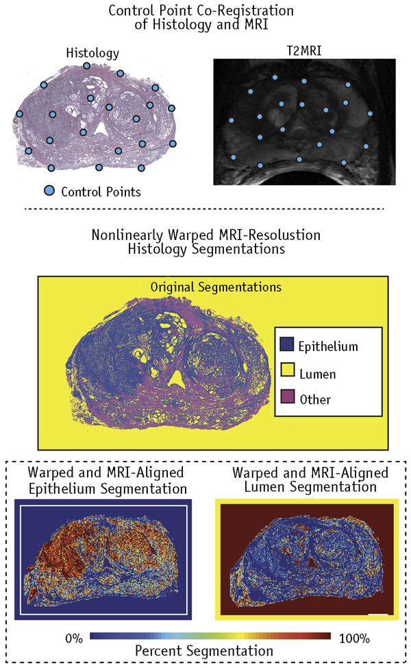
Digitized histology was annotated by a fellowship-trained urologic pathologist (KAI) using the Gleason grading system updated to distinguish cribriform from noncribriform glands within G4 tumors (25). Cribriform cancer was distinguished from fused gland cancer because of the notable difference in outcome between the 2 types of G4 tumors (26). For the purposes of this analysis, both G4 tumor types and G5 tumors were grouped into a high-grade classification. Examples of scored samples are shown in Figure 1. Regions of solid color indicating disease severity were manually annotated on the high-resolution histologic images using a Microsoft Surface Pro 4 (Microsoft, Seattle, WA). Automated segmentation of the lumen and epithelium(27) was performed using custom code developed in MATLAB (The MathWorks, Natick, MA). The algorithm used raw self explanatory values and binary morphologic operations to create tissue masks for the lumen, epithelium, and other tissue. An example of the automated prostate segmentation is shown in Figure 2. This study included 210 whole-mount slides from the 39 patients.

Fig. 2.

Control point co-registration of histology to T2 magnetic resonance image. The automated segmentation of the lumen and epithelium was nonlinearly warped and down-sampled to the magnetic resonance imaging (MRI) resolution for a one-to-one comparison.

Tissue segmentation validation

To determine whether our custom software performed similarly to a human, 18 samples of different Gleason grades including normal, G3, G4, and atrophy from 11 patients were manually annotated and confirmed by a pathologist (KAI) with urologic pathology fellowship training. The lumen and epithelium densities were then compared with the densities calculated by the automated segmentation software using a Pearson correlation.

Comparison of histologic segmentation values between Gleason grades

The mean histologic segmentation values for the lumen and epithelium were computed across each annotated tumor region identified by our pathologist. Statistical comparisons were performed between lesion grades using a t test.

Histologic co-registration

Digitized samples were co-registered to the T2-weighted image using software and techniques previously published (23). A control point co-registration was applied using manually placed analogous points in each modality. Points were placed along the boundaries of the organ and on clearly identifiable landmarks within the organ. Between 20 and 50 control points were placed on each slide. The whole-mount slide and the control points were down-sampled to MRI resolution. A nonlinear spatial transform was calculated from the control points using MATLAB’s “fitgeotrans” function, and the transformation matrix was saved. The transform was then applied using the “imwarp” function. A local weighted-means transform was used for the histology to account for the nonuniform distortions caused by the endorectal coil compressing the organ, bringing the histology into the MRI space (Fig. 2). This nonlinear spatial transform was likewise applied to the digitized pathologic annotation and segmentations (Fig. 2) (23, 28). A nearest-neighbor transform was used for the pathologist’s annotations to retain the integer values.

Co-registration validation

To validate the control point co-registration, the nonlinear control pointederived transforms were compared with a known spatial transform, which altered the size, rotation, and skew of 5 whole-mount histologic slides containing pathologist-annotated regions. Analogous control points were placed on both the original slide and the slide with the known transform. The imwarp function was then applied to the original slides and the expert annotations. A Dice coefficient was calculated to quantify the similarity between the known and calculated transformed annotations.

Machine-learning model optimization

The MP-MRI lesion values were used as the input variables to a machine-learning algorithm (described later) trained with the aligned lumen and epithelium densities derived from pathology. A learning curve was generated to determine the ideal number of patients required for a stable model. Models were iteratively trained, increasing the number of patients from 1 to 29, with 10 iterations performed at each step. Patients were randomly selected at each iteration, and the models were trained lesion-wise. Lesions included G3 or higher and benign atrophy. Data points were corrected for patient number and slice number. A plot of root-mean-square error versus number of lesions included in the training set was created, and a curve of the form shown in equation 1 was fit to the data, in which a, b, and g are constants and N is the number of data points used to train the algorithm (29). To determine the optimal lesion number, the limit of the learning curve as N approached infinity was determined. The curve was then evaluated to determine the point at which 99% of the calculated limit was achieved, resulting in the optimal number of training data points included.

$$Error=\alpha \ast N^{\beta }+\gamma$$ (1)

Group assignment

On the basis of the learning-curve analysis outlined earlier, it was determined that 10 patients were sufficient for a stable training dataset (as is discussed in the “Results” section). Patients were assigned to 3 class-balanced groups: 2 training sets of 10 patients and 1 test group of 19 patients. Tumor burden was balanced across the 3 cohorts. The total number of lesions was calculated on a per-patient basis; patients were then randomly permuted, with tracking of the total tumor burden of each cohort. Patients with G5 tumors were shuffled and assigned such that the distribution was constant across all cohorts. This process was repeated recursively for G4 and G3 tumors.

Input feature set and analysis

Six MP-MRI contrasts were used as the input set: intensity-normalized T2, delta T1, B=0 diffusion weighted image, and ADC calculated with 3 b-value combinations (0–1000, 1000–2000, and 500–2000), each sensitive to different tissue diffusion characteristics (23). Median MP-MRI values were calculated within each pathologist-annotated region of interest, and the feature set was then z normalized. To determine the predictive power of each MP-MRI feature, we performed a recursive greedy analysis for each training cohort. The correlation between each feature and epithelium and lumen density was also measured. To additionally determine the level of collinearity, a correlation analysis was performed on each input feature set for cohorts 1 and 2.

Machine-learning approach

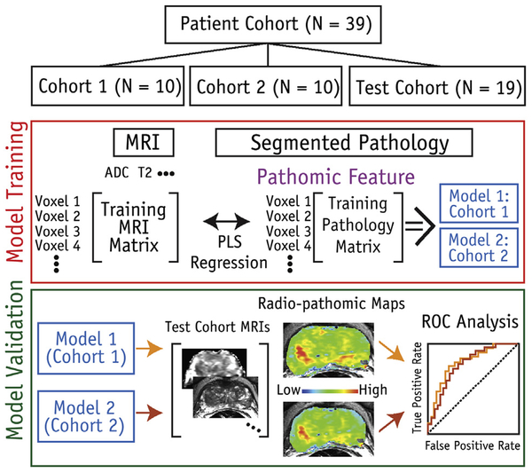
The median MP-MRI values and corresponding pathologically derived lumen and epithelium densities were used to train partial least-squares regression models for each training cohort of 10 patients. Each model was generated using 1 latent variable. Separate fits were calculated for the lumen and epithelium. The resulting models from both cohorts were then applied to the test cohort as outlined later. A schematic of the machine-learning protocol is shown in Figure 3.

Fig. 3.

Diagram of machine-learning protocol used in study. Patients were stratified into 1 of 3 cohorts (2 independent training cohorts and 1 test cohort). Magnetic resonance imaging (MRI) values were used as input features to predict epithelium and lumen density. Two independent models were produced using the 2 training sets. Both derived models were then applied to the same test cohort. Abbreviations: ADC = apparent diffusion coefficient; PLS = partial least squares; ROC = receiver operating characteristic.

Radio-pathomic mapping

The resulting partial least-squares models were applied to the MP-MRI scans from each of the 19 patients in the test cohort. Predicted values of epithelium and lumen density were calculated voxel-wise for each model. An image was then generated from the predicted values in the space defined by the T2 image (Fig. 3). No spatial filters were applied to the resulting maps prior to display.

Comparison of predicted values between Gleason grades

The average predicted lumen and epithelium values from the radio-pathomic maps were calculated from the pathologist-annotated regions of different Gleason grades. These values were then compared statistically using a t test for G4 or higher versus G3 or lower tumors. Analogous lumen and epithelium density values were statistically compared likewise from the actual histologic segmentations.

Receiver operating characteristic analysis

To quantify the performance of the radio-pathomic models, a receiver operating characteristic (ROC) analysis was performed lesion-wise on the test dataset, evaluating each model’s ability to differentiate G4+ from G3- tumors. The ROC curves were statistically tested between models to determine whether the performance varied statistically.

Results

Segmentation accuracy

The segmentation accuracy results are shown in Figure E1 (available online at www.redjournal.org). The lumen and epithelium both showed high correlation between manual and computational segmentation (R = 0.99 and R = 0.72, respectively; P < .001).

Co-registration accuracy

The Dice coefficient analysis revealed 94.5% overlap, indicating that the control point warping technique effectively transforms the pathologist’s expert annotations and histologic segmentations into the MRI space (Fig. E2; available online at www.redjournal.org).

Input feature set and analysis

The MP-MRI features ranked by predictive power are shown in Table E3 (available online at www.redjournal. org), in which the contributions of each feature varied slightly between cohorts and the histologic feature of interest. Each feature was significantly correlated with both the lumen and epithelium for both models (P < .001). We found that ADC calculated with b values of 0 to 1000 was highly predictive in all 4 conditions; delta T1 was also highly predictive in 3 of 4 conditions. The cross correlation of the 6 input features is shown in Figure E3 (available online at www.redjournal.org). As expected, the ADC features showed a high degree of correlation. An interesting finding was that delta T1 provided the most diverse source of information comparatively.

Model cross validation

The results plotting root-mean-square error versus number of lesions are shown in Figure E4 (available online at www.redjournal.org). The lumen curve reached 99% of the calculated limit at 320 lesions, which equates to about 10 patients. Epithelium values stabilized sooner. Radio-pathomic maps of epithelium density resulting from models trained with 2, 4, 6, 8, and 10 patients are shown in Figure E5 (available online at www.redjournal.org). The contrast improved as patients were added to the training dataset, and the maps stabilized at 10 patients, analogous to the learning curve.

Radio-pathomic maps

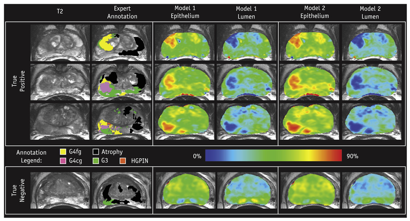
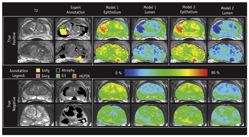
Predicted lumen and epithelium density values were generated for each of the 19 patients in the test cohort and mapped voxel-wise. Figure 4 shows radio-pathomic maps of lumen and epithelium density from 4 representative patients, where regions of increased epithelium density and decreased lumen density corresponded with pathologist-annotated high-grade tumors for both models. Figure 5 shows 4 additional sets of radio-pathomic maps compared with the aligned pathologist annotations.

Fig. 4.

Examples of the resulting radio-pathomic maps of lumen and epithelium density generated with each model compared with the expert pathologist annotation overlaid on the T2 magnetic resonance image. The high-grade lesions are highlighted as increased epithelium density and decreased lumen density, analogous to the actual histology (0%−90% scale). The 3 patients on the top had high-grade tumors (true positives), while the patient on the bottom had a region of Gleason grade 3 (G3), not highlighted by the radio-pathomic maps (true negative). Abbreviations: G4cg = Grade 4 cribriform gland; G4fg = Grade 4 fused gland; HGPIN = high-grade intraepithelial neoplasia.

Fig. 5.

Additional examples of the resulting radio-pathomic maps of lumen and epithelium density generated with each model compared with the expert pathologist annotation overlaid on the T2 magnetic resonance image (0%−90% scale). The 2 patients on the top had high-grade tumors (true positives), while the 2 patients on the bottom had true-negative findings. Abbreviation: HGPIN = high-grade intraepithelial neoplasia.

Comparison of predicted values between Gleason grades

The t test comparison of radio-pathomic map values between G4+ and G3- tumors in the test cohort was significant for lumen density in models 1 and 2 (P < .001) and epithelium density in models 1 and 2 (P < .01). The results are shown in Figure E6 (available online at www.redjournal.org). and compared with the actual histologic segmentations within analogous regions (both significantly different with P < .001).

ROC analysis

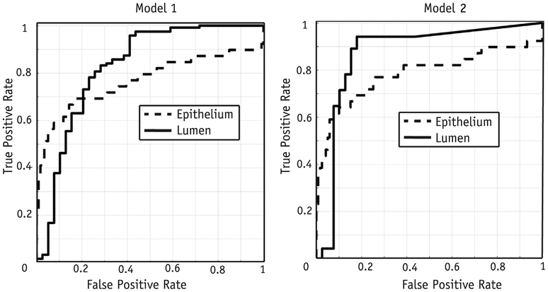
Results of the ROC analysis using radio-pathomic map values to differentiate high-grade cancer (G4+) are shown in Figure 6, in which model 1 had an epithelium area under the curve (AUC) of 0.76 ± 0.11 and lumen AUC of 0.82 ± 0.09. Model 2 had an epithelium AUC of 0.78 ± 0.10 and lumen AUC of 0.86 ± 0.08. The ROC curves compared between models 1 and 2 for both the lumen and epithelium were not statistically different (P = .32 and P = .77, respectively). Lumen density maps outperformed epithelium density maps, mirroring the results seen in the aforementioned t test.

Fig. 6.

Receiver operating characteristic analysis of the performance of models 1 and 2 differentiating high-grade cancer in the test cohort. The model 1 area-under-the-curve values for the lumen and epithelium were 0.82 ± 0.09 and 0.76 ± 0.11, respectively. The model 2 performance evaluated in the test cohort showed area-under-the-curve values for the lumen and epithelium of 0.86 ± 0.08 and 0.78 ± 0.10, respectively.

Discussion

We present a technique, termed “radio-pathomic mapping,” that generates predictive maps of prostate cancer pathologic features in MRI space. The steps necessary for generating these maps were extensively validated by subanalyses that (1) validated the automatic segmentation of prostate histology, (2) determined the ideal number of data points included in the training datasets, and (3) verified nonlinear alignment transforms against known transforms. We determined that rad-path datasets from 10 patients were sufficient to train a stable model and split our sample of 39 patients into 2 training cohorts and 1 test cohort. Separate models were derived from each training cohort and applied to the test cohort to calculate predicted epithelium and lumen density voxel-wise values using MP-MRI alone. Predicted densities were then extracted from pathologist defined regions of interest brought into the MRI space and compared statistically. We found that the maps were visually interpretable and statistically separated G4+ from G3- prostate cancer.

The treatment and staging of prostate cancer could stand to benefit from improved noninvasive imaging, especially in the field of image guided radiation therapy. The current standard of care involves irradiating the whole gland with a single prescription dose. Active investigations are ongoing that focus on the integration of MP-MRI into radiation treatment planning both in the prostate (30) and in other organs (31). Several limitations prevent direct implementation, such as the subjectivity of MP-MRI interpretation, the subjectivity of tumor boundaries, and the limited direct correlation with histopathologic data. Radio-pathomic mapping may provide additional information in MRI space for targeted radiation therapy.

The presence of G4 cancer is a critical barrier for driving prostate cancer treatment (32). This study shows that radio-pathomic maps of epithelium and lumen density effectively discriminate G4+ tumors. Examples of patients with both G4+ and G3 tumors are shown in Figures 4 and 5, in which high-grade tumors are readily seen on both the epithelium and lumen density maps derived from each model. Combined with clinical imaging, radiologists may be able to filter out false positives and use these maps to increase their confidence in clinical decision making. Validating this hypothesis will require a full reader study.

There are several potential sources of error intrinsic to radio-pathomic mapping. The histologic slides were cut at 10 μm, sampling only a small portion of the full 4-mm MRI slice. We used custom patient-specific prostate slicing jigs to optimize the orientation of tissue sectioning and included on average 5 slices per patient. This is a potential avenue for future research, in which perturbations in MRI orientation and co-registrations could be intentionally induced to determine the downstream consequences on the radio-pathomic algorithm.

There are known sources of interobserver variability in prostate pathology grading that may also contribute error to our ground truth. One recent study compared annotations from 23 genitourinary pathologists and found a consensus (80% agreement) in 78% of cases (33). A similar study comparing 2 pathologists’ observations over a wider range of disease found moderate agreement between pathologists (34). It is therefore possible that both our models and ROC results would vary given a different pathologist’s annotations. In its current form, our technique correctly identifies prostate cancer annotated by our pathologist using data collected on our MRI system. While we believe this technique will generalize beyond our institution, a multi-institutional study should be performed varying the MRI scanner and the pathologist annotating the ground truth.

The Prostate Imaging Reporting and Data System (PI-RADS) system used for standardized interpretation of prostate MRI scans weights different imaging characteristics differently depending on where in the prostate a lesion is located. This study combined lesions from both zones into 1 training and test dataset. Future studies should be performed to determine the spatial dependence of the radio-pathomic methodology.

In conclusion, we present a radio-pathomic approach for generating predictive maps of prostate cancer histologic features. Our technique highlights and stratifies G4+ tumors and generates 2 new interpretable image contrasts þ of epithelium and lumen density. These maps may have important relevance for personalized radiation dose-painting strategies and detection of clinically relevant prostate cancer.

References

- 1.Siegel RL, Miller KD, Jemal A. Cancer statistics, 2016. CA Cancer J Clin 2016;66:7–30. [DOI] [PubMed] [Google Scholar]
- 2.Klotz L, Vesprini D, Sethukavalan P, et al. Long-term follow-up of a large active surveillance cohort of patients with prostate cancer. J Clin Oncol 2015;33:272–277. [DOI] [PubMed] [Google Scholar]
- 3.Hambrock T, Somford DM, Huisman HJ, et al. Relationship between apparent diffusion coefficients at 3.0-T MR imaging and Gleason grade in peripheral zone prostate cancer. Radiology 2011;259:453–461. [DOI] [PubMed] [Google Scholar]
- 4.Vos EK, Kobus T, Litjens GJ, et al. Multiparametric magnetic resonance imaging for discriminating low-grade from high-grade prostate cancer. Invest Radiol 2015;50:490–497. [DOI] [PubMed] [Google Scholar]
- 5.Tewes S, Mokov N, Hartung D, et al. Standardized reporting of prostate MRI: Comparison of the Prostate Imaging Reporting and Data System (PI-RADS) version 1 and version 2. PLoS One 2016;11: e0162879. [DOI] [PMC free article] [PubMed] [Google Scholar]
- 6.Vargas HA, Hotker AM, Goldman DA, et al. Updated prostate imaging reporting and data system (PIRADS v2) recommendations for the detection of clinically significant prostate cancer using multiparametric MRI: Critical evaluation using whole-mount pathology as standard of reference. Eur Radiol 2016;26:1606–1612. [DOI] [PMC free article] [PubMed] [Google Scholar]
- 7.Marks L, Young S, Natarajan S. MRI-ultrasound fusion for guidance of targeted prostate biopsy. Curr Opin Urol 2013;23:43–50. [DOI] [PMC free article] [PubMed] [Google Scholar]
- 8.Chang JH, Lim Joon D, Nguyen BT, et al. MRI scans significantly change target coverage decisions in radical radiotherapy for prostate cancer. J Med Imaging Radiat Oncol 2014;58:237–243. [DOI] [PubMed] [Google Scholar]
- 9.Aerts HJ, Velazquez ER, Leijenaar RT, et al. Decoding tumour phenotype by noninvasive imaging using a quantitative radiomics approach. Nat Commun 2014;5:4006. [DOI] [PMC free article] [PubMed] [Google Scholar]
- 10.Gillies RJ, Kinahan PE, Hricak H. Radiomics: Images are more than pictures, they are data. Radiology 2016;278:563–577. [DOI] [PMC free article] [PubMed] [Google Scholar]
- 11.Litjens GJ, Elliott R, Shih NN, et al. Computer-extracted features can distinguish noncancerous confounding disease from prostatic adeno-carcinoma at multiparametric MR imaging. Radiology 2016;278:135–145. [DOI] [PMC free article] [PubMed] [Google Scholar]
- 12.McGarry SD, Hurrell SL, Kaczmarowski AL, et al. Magnetic resonance imaging-based radiomic profiles predict patient prognosis in newly diagnosed glioblastoma before therapy. Tomography 2016;2: 223–228. [DOI] [PMC free article] [PubMed] [Google Scholar]
- 13.Artan Y, Haider MA, Langer DL, et al. Prostate cancer localization with multispectral MRI using cost-sensitive support vector machines and conditional random fields. IEEE Trans Image Process 2010;19: 2444–2455. [DOI] [PubMed] [Google Scholar]
- 14.Fehr D, Veeraraghavan H, Wibmer A, et al. Automatic classification of prostate cancer Gleason scores from multiparametric magnetic resonance images. Proc Natl Acad Sci U S A 2015;112:E6265–E6273. [DOI] [PMC free article] [PubMed] [Google Scholar]
- 15.Rampun A, Zheng L, Malcolm P, et al. Computer-aided detection of prostate cancer in T2-weighted MRI within the peripheral zone. Phys Med Biol 2016;61:4796–4825. [DOI] [PubMed] [Google Scholar]
- 16.Shah V, Pohida T, Turkbey B, et al. A method for correlating in vivo prostate magnetic resonance imaging and histopathology using individualized magnetic resonance-based molds. Rev Sci Instrum 2009;80: 104301. [DOI] [PMC free article] [PubMed] [Google Scholar]
- 17.Nguyen HS, Milbach N, Hurrell SL, et al. Progressing bevacizumab-induced diffusion restriction is associated with coagulative necrosis surrounded by viable tumor and decreased overall survival in patients with recurrent glioblastoma. AJNR Am J Neuroradiol 2016;37:2201–2208. [DOI] [PMC free article] [PubMed] [Google Scholar]
- 18.Langer DL, van der Kwast TH, Evans AJ, et al. Prostate tissue composition and MR measurements: Investigating the relationships between ADC, T2, K(trans), v(e), and corresponding histologic features. Radiology 2010;255:485–494. [DOI] [PubMed] [Google Scholar]
- 19.Tanimoto A, Nakashima J, Kohno H, et al. Prostate cancer screening: The clinical value of diffusion-weighted imaging and dynamic MR imaging in combination with T2-weighted imaging. J Magn Reson Imaging 2007;25:146–152. [DOI] [PubMed] [Google Scholar]
- 20.Jenkinson M, Bannister P, Brady M, et al. Improved optimization for the robust and accurate linear registration and motion correction of brain images. Neuroimage 2002;17:825–841. [DOI] [PubMed] [Google Scholar]
- 21.Sood A, Jeong W, Peabody JO, et al. Robot-assisted radical prostatectomy: Inching toward gold standard. Urol Clin North Am 2014;41: 473–484. [DOI] [PubMed] [Google Scholar]
- 22.Menon M, Hemal AK, Team VIP. Vattikuti Institute prostatectomy: A technique of robotic radical prostatectomy: Experience in more than 1000 cases. J Endourol 2004;18:611–619; discussion 619. [DOI] [PubMed] [Google Scholar]
- 23.Hurrell SL, McGarry SD, Kaczmarowski A, et al. Optimized b-value selection for the discrimination of prostate cancer grades, including the cribriform pattern, using diffusion weighted imaging. J Med Imaging (Bellingham) 2018;5:011004. [DOI] [PMC free article] [PubMed] [Google Scholar]
- 24.Cox RW. AFNI: Software for analysis and visualization of functional magnetic resonance neuroimages. Comput Biomed Res 1996;29:162–173. [DOI] [PubMed] [Google Scholar]
- 25.Epstein JI, Egevad L, Amin MB, et al. The 2014 International Society of Urological Pathology (ISUP) Consensus Conference on Gleason grading of prostatic carcinoma: Definition of grading patterns and proposal for a new grading system. Am J Surg Pathol 2016;40:244–252. [DOI] [PubMed] [Google Scholar]
- 26.Iczkowski KA, Torkko KC, Kotnis GR, et al. Digital quantification of five high-grade prostate cancer patterns, including the cribriform pattern, and their association with adverse outcome. Am J Clin Pathol 2011;136:98–107. [DOI] [PMC free article] [PubMed] [Google Scholar]
- 27.Kwak JT, Sankineni S, Xu S, et al. Correlation of magnetic resonance imaging with digital histopathology in prostate. Int J Comput Assist Radiol Surg 2016;11:657–666. [DOI] [PMC free article] [PubMed] [Google Scholar]
- 28.LaViolette PS, Mickevicius NJ, Cochran EJ, et al. Precise ex vivo histological validation of heightened cellularity and diffusion-restricted necrosis in regions of dark apparent diffusion Neuro Oncol 2014;16:1599–1606. [DOI] [PMC free article] [PubMed] [Google Scholar]
- 29.Hess KR, Wei C. Learning curves in classification with microarray data. Semin Oncol 2010;37:65–68. [DOI] [PMC free article] [PubMed] [Google Scholar]
- 30.Lips IM, van der Heide UA, Haustermans K, et al. Single blind randomized phase III trial to investigate the benefit of a focal lesion ablative microboost in prostate cancer (FLAME-trial): Study protocol for a randomized controlled trial. Trials 2011;12:255. [DOI] [PMC free article] [PubMed] [Google Scholar]
- 31.Hall WA, Bergom C, Thompson RF, et al. Precisioncoefficient in 7 cases of high-grade glioma. oncology and genomically guided radiation therapy: A report from the American Society for Radiation Oncology/American Association of Physicists in Medicine/National Cancer Institute Precision Medicine Conference. Int J Radiat Oncol Biol Phys 2018;101:274–284. [DOI] [PubMed] [Google Scholar]
- 32.Epstein JI, Zelefsky MJ, Sjoberg DD, et al. A contemporary prostate cancer grading system: A validated alternative to the Gleason score. Eur Urol 2016;69:428–435. [DOI] [PMC free article] [PubMed] [Google Scholar]
- 33.Kweldam CF, Nieboer D, Algaba F, et al. Gleason grade 4 prostate adenocarcinoma patterns: An interobserver agreement study among genitourinary pathologists. Histopathology 2016;69:441–449. [DOI] [PubMed] [Google Scholar]
- 34.Ozkan TA, Eruyar AT, Cebeci OO, et al. Interobserver variability in Gleason histological grading of prostate cancer. Scand J Urol 2016;50: 420–424. [DOI] [PubMed] [Google Scholar]
Associated Data
This section collects any data citations, data availability statements, or supplementary materials included in this article.