A Dynamic Bayesian Observer Model Reveals Origins of Bias in Visual Path Integration

SUMMARY

Path integration is a strategy by which animals track their position by integrating their self-motion velocity. To identify the computational origins of bias in visual path integration, we asked human subjects to navigate in a virtual environment using optic flow, and found that they generally traveled beyond the goal location. Such a behavior could stem from leaky integration of unbiased self-motion velocity estimates, or from a prior expectation favoring slower speeds that causes velocity underestimation. Testing both alternatives using a probabilistic framework that maximizes expected reward, we found that subjects’ biases were better explained by a slow-speed prior than imperfect integration. When subjects integrate paths over long periods, this framework intriguingly predicts a distance-dependent bias reversal due to build-up of uncertainty, which we also confirmed experimentally. These results suggest that visual path integration in noisy environments is limited largely by biases in processing optic flow rather than by leaky integration.

ETOC BLURB

Humans are typically biased while navigating by integrating their self-motion. Using virtual reality and probabilistic modeling, Lakshminarasimhan et al. demonstrate that systematic errors in visual path integration originate from the combined influence of a slow-velocity prior and growing position uncertainty.

INTRODUCTION

The world is inherently noisy and dynamic. To act successfully, we must continuously monitor our sensory inputs, gather evidence in favor of potential actions, and make subjectively good decisions in the face of uncertain evidence. Traditional binary decision tasks lack the temporal richness to shed light on continuous behaviors in demanding environments (Lee et al., 2014; Pitkow and Angelaki, 2017). Newer “continuous psychophysics” methods (Bonnen et al., 2015; Mulligan et al., 2013) can constrain models much more rapidly, and can be elaborated to simulate real-world challenges. Here we develop a naturalistic visuomotor virtual navigation task with controllable sensory uncertainty, and provide a unified framework to understand how dynamic perceptual information is combined over time. We then use this framework to understand the origins of bias in path integration – a natural computation that involves sensory perception, evidence accumulation, and spatial cognition.

Path integration is a navigation strategy used to maintain a sense of position solely by integrating self-motion information. Humans and animals are capable of path integrating (Alyan and Jander, 1994; Benhamou, 1997; Collett and Collett, 2000; Etienne, 1992; Golledge, 1999; Seguinot et al., 1998), albeit often with systematic errors (or biases). Biases have been observed in many species under a variety of experimental conditions involving visual (Bakker et al., 2001; Frenz and Lappe, 2005; Lappe and Frenz, 2009; Redlick et al., 2001) and/or body-based (Jürgens et al., 1999; Klatzky et al., 1990; Loomis et al., 1993) (e.g. vestibular, proprioceptive) self-motion cues, yet their origins are not fully understood.

Broadly speaking, path integration entails two stages – estimating one’s self-motion, and integrating that estimate over time. Most previous accounts of behavioral biases in path integration implicate the latter, arguing for suboptimal integration of movement velocity that produces errors that increase with time (Mittelstaedt and Glasauer, 1991; Mittelstaedt and Mittelstaedt, 2001; Vickerstaff and Di Paolo, 2005) or distance (Bergmann et al., 2011; Brossard et al., 2016; Lappe et al., 2007, 2011). However, past modeling approaches were dominated by attempts to fit empirical functions using only subjects’ final states at the end of the integration process, without considering the performance constraints imposed by noise in the sensory inputs. This has led to the view that bias in path integration is due to leaky integration – a severely suboptimal strategy that is inconsistent with studies in other domains demonstrating statistically optimal behavior in static and dynamic binary tasks (Bogacz and Bogacz, 2007; Brunton et al., 2013; Ernst et al., 2012; Fiser et al., 2010; Issen et al., 2015; Jogan and Stocker, 2013).

An alternative explanation is that the bias stems from errors in sensory estimates – e.g., from bias in velocity estimation or from incorrectly accumulating perceptual uncertainty over time. For example, human judgement of retinal speed is known to be biased and this is well explained by a Bayesian observer model with a slow-speed prior (Hürlimann et al., 2002; Sotiropoulos et al., 2014; Stocker and Simoncelli, 2006; Weiss et al., 2002). If a similar prior biases our judgement of self-motion velocity, this will naturally lead to path integration biases even if the integration itself is perfect. This alternative explanation has been invoked previously to explain bias in integrating passive angular rotations (Jürgens and Becker, 2006), and proposed to be important for path integration in general (Petzschner and Glasauer, 2011). However, this proposal has never been rigorously tested against explanations based on leaky integration. These two alternatives have very different implications for neural models of evidence accumulation under uncertainty, so it is important to distinguish them. Finally, to our knowledge, past studies of path integration considered integration of either angles or distance but not both. Therefore, it is unclear if those findings would generalize to navigation in the real world.

To more directly determine whether bias in path integration under naturalistic conditions stems mainly from a slow-speed prior or suboptimal integration, we tested human subjects on a task in which they navigated within a horizontal plane using sparse optic flow. We found that subjects underestimated both linear and angular displacements when navigating short distances. We analysed these data using a mathematical theory that includes components for sensory processing, integration dynamics, and decision-making. Our analysis revealed that the behavioral errors can be explained by a model in which subjects maximized their expected reward under the influence of a slow-speed prior, rather than by leaky integration of unbiased velocity estimates. This result was confirmed in a separate experiment in which we tested the predictions of both models by manipulating the reliability and the range of optic flow. In addition, when extended to longer distance scales, the model predicts a potential reversal in the pattern of bias from overshooting to undershooting due to build-up of uncertainty, and we also confirmed this prediction experimentally. These findings suggest that human subjects can maintain a dynamic probabilistic representation of their location while navigating, and their ability to path integrate is limited largely by brain structures that process self-motion rather than by circuits that integrate velocity estimates based on optic flow.

RESULTS

We asked human subjects to perform a visual navigation task in which they used a joystick to steer to a cued target location in a virtual environment devoid of allocentric reference cues (Fig 1A, Movies S1-S2, Methods). At the beginning of each trial, a circular target blinked briefly (~1s) at a random location on the ground plane, after which it disappeared and the joystick controller was activated. The joystick had two degrees of freedom that controlled forward and angular velocities, allowing the subject to steer freely in two dimensions (Fig 1B). Subjects were instructed to stop steering when they believed their position fell within the target, but did not receive any performance-related feedback. Target locations were varied randomly across trials and were uniformly distributed over the ground plane area within the subject’s field of view (Fig 1C – top). The subject’s movement trajectory was recorded throughout each trial (Fig 1C – bottom).

Figure 1. Task structure and behavioral response.

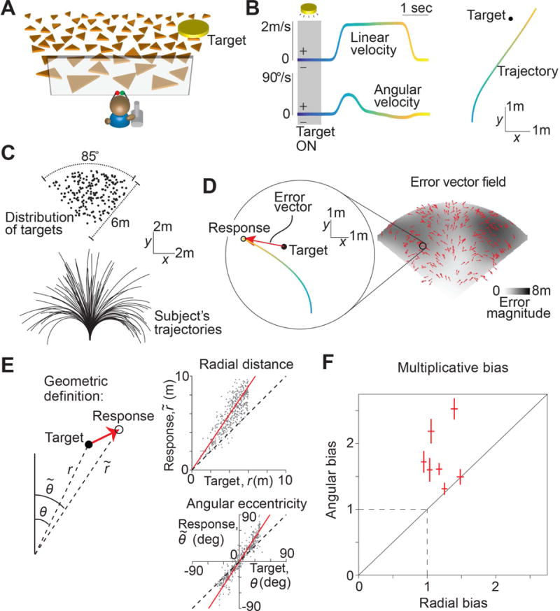
A. Subjects use a joystick to navigate to a cued target (yellow disc) using optic flow cues generated by ground plane elements (orange triangles). The ground plane elements appeared transiently at random orientations to ensure that they cannot serve as spatial or angular landmarks (Methods). B. Left: The time course of linear (top) and angular (bottom) speeds during one example trial. Time is also encoded by line color. Right: Aerial view of the subject’s spatial trajectory during the same trial. C. Top: Aerial view of the spatial distribution of target positions across trials. Bottom: Subject’s movement trajectories during a representative subset of trials. D. Left: Target location (solid black) and subject’s steering response (colored as in B) during a representative trial. Red arrow represents the error vector. Right: Vector field denoting the direction of errors across trials. The tail of each vector is fixed at the target location and vectors were normalized to a fixed length for better visibility. The grayscale background shows the spatial profile of the error magnitude. E. Top right: Comparison of the radial distance $\stackrel{\sim }{r}$ of the subject’s response (final position) against radial distance r of the target across all trials for one subject. Bottom right: Angular eccentricity of the response $\stackrel{\sim }{\theta }$ vs. target angle θ. Black dashed lines have unity slope and the red solid lines represent slopes of the regression fits. Left: Geometric meaning of the quantities in the scatter plots. F. Radial and angular biases were quantified as the slopes of the corresponding regressions and plotted for individual subjects. Error bars denote 95% confidence intervals of the respective slopes. Dashed lines indicate unbiased radial or angular position responses. Solid diagonal line has unit slope. See also Figures S1-S2 and Movies S1-S2.

Behavioral data

The subject’s ‘response location’ was given by their stopping position at the end of each trial. We quantified behavioral error on each trial by comparing the response location against the target location. Figure 1D (left) shows an aerial view of the target location and one subject’s trajectory during a representative trial. On this trial, the error vector points radially outward and away from straight ahead, implying that the subject overshot the target both in terms of the net distance moved as well as the net angle rotated. The vector field of errors across all trials revealed a qualitatively similar pattern of errors throughout the experiment (Fig 1D – right).

To quantify these errors, we separately compared the radial distance and angular eccentricity of the target to those of the subject’s response location in each trial. We found a systematic bias underlying the response errors in both quantities: this subject consistently traveled a greater distance and rotated through a greater angle than necessary (Fig 1E). We observed similar biases across subjects (Fig S1A), and these biases were well described by a simple linear model with multiplicative gain scaling, rather than an additive shift, of the subjects’ estimates of their net displacement and rotation (mean coefficient of determination, across subjects – distance: 0.70 ± 0.12, angle: 0.92 ± 0.11). Moreover, this multiplicative model was able to capture ~95% of the variance explained by more complicated nonlinear models (see legend of Fig S1A). Therefore, instead of quantifying bias in units of distance and angle, we used the slopes of the corresponding linear regressions (i.e., the gain) as a measure of bias in radial distance and angle for each subject. In this scheme, slopes greater than and less than unity correspond to overshooting and undershooting respectively, while unity (not zero) slope corresponds to unbiased performance. Both radial and angular biases were significantly greater than unity across subjects (Fig 1F, mean distance bias (± standard error), Γ_r = 1.19 ± 0.07, = 4.1 × 10⁻², t-test; mean angle bias, Γ_θ = 1.78 ± 0.16, p = 2.8 × 10⁻³).

We varied target locations across trials to preclude the use of strategies based only on movement duration. Nevertheless, subjects may have been encouraged to use such a strategy due to the inherent relationship between distance and time. To test this, we randomly interleaved trials in which we removed all ground plane elements, thereby eliminating optic flow. The correlation between target and response locations dropped substantially in these trials (Fig S1B), implying that subjects relied heavily on optic flow cues, rather than a mental clock, to perform the task.

We allowed subjects to freely control their velocity at all times and found modest variability in average velocity across trials. This trial-by-trial variability in velocity was uncorrelated with trial-by-trial variability in subjects’ radial and angular position biases (Fig S1C), suggesting that movement velocity within the range we observed does not influence subjects’ path integration errors during self-generated movement. Such a velocity-independent bias can arise if bias in velocity estimation is multiplicative, and we quantitatively model and test this phenomenon later. Velocities varied across time differently for different subjects as well: four of the seven subjects used a serial strategy, first rotating and then moving straight ahead to reach the target (Fig S2A, B), while the remaining subjects traveled along curvilinear trajectories. Subjects with both strategies had comparable radial and angular biases (Fig S2C), suggesting that they do not benefit from integrating the angular and linear components separately. This finding also shows that overshooting is not restricted to cases in which subjects make curvilinear trajectories.

Finally, we introduced angular landmarks in the environment by displaying a distant mountainous background (Fig S2D). This manipulation did not alter the radial bias, but eliminated angular bias almost completely (Γ_r = 1.29 ± 0.08, Γ_θ = 1.1 ± 0.04; Fig S2E). This suggests that biases measured in the absence of landmarks reflect errors in spatial perception rather than problems associated with motor control. To further validate this, we conducted an additional experiment in which we passively transported subjects over trajectories that passed through the targets at a constant velocity, thereby eliminating motor control (Methods, Fig S2F). Subjects simply pressed a button to indicate when they believed they had reached the target. Again we observed overshooting that scaled linearly with the radial distance of the target (Γ_r = 1.38 ± 0.1; Fig S2G). Note that a delay in pressing the button would produce an identical bias at all distances (i.e., additive bias) and thus cannot explain the above result.

Together, these data suggest that subjects overshoot when using optic flow to navigate modest distances regardless of the precise speed or curvature of the trajectory, and this bias is due to a systematic error in the subject’s perception, not action.

Dynamic Bayesian Observer model

Past studies have attributed biases in path integration to leaky integration (Lappe et al., 2007, 2011; Mittelstaedt and Glasauer, 1991; Mittelstaedt and Mittelstaedt, 2001; Vickerstaff and Di Paolo, 2005). According to those behavioral models, subjects forget part of their movement history, leading to sub-additive accumulation of self-motion information. Consequently, they underestimate their distance moved and end up traveling further than necessary, overshooting the target. We asked whether the overshooting could instead result from accurate integration of inaccurate, biased velocity estimates. Specifically, if subjects were to underestimate their linear and/or angular movement velocities, accurate integration might yet lead to overshooting. In fact, human subjects are known to underestimate retinal velocities, and those effects have been successfully attributed to a slow-speed prior using Bayesian theories (Hürlimann et al., 2002; Sotiropoulos et al., 2014; Stocker and Simoncelli, 2006; Weiss et al., 2002).

We hypothesized that such a slow-speed prior might also underlie the biases observed in our experiments. We tested this possibility against the alternative of leaky temporal integration using the framework of a dynamic Bayesian observer model. In this framework, we explicitly model the subject’s belief, i.e. the subjective posterior distribution, which is the posterior over position given its model assumptions. This is computed across two stages: combining noisy optic flow input with a prior belief to compute the posterior over self-motion velocity (inference step), and integrating the resulting posterior with a constant leak rate (integration step). Since the position estimate is uncertain, we used this framework to identify model parameters that maximized the expected reward, a quantity that takes both the mean and uncertainty in position into account. Although we will shortly show that the above behavioral results can be understood purely in terms of a bias in subjects’ mean position estimates, we will also show in a later section that uncertainty plays a pivotal role in influencing responses when navigating larger distances.

Since position is computed by integrating velocity, bias in position estimates can originate either from bias in velocity estimation or from imperfect integration. We modeled the distinction between these two hypotheses within the proposed framework by manipulating the shape of the prior to be exponential or uniform, and the nature of integration to be perfect or leaky (Fig 2). At one extreme, the combination of an exponential prior and perfect integrator would attribute path integration bias entirely to underestimation of self-motion velocity. At the other extreme, a uniform prior would yield unbiased velocity estimates which, if integrated with leak, could also lead to a bias as proposed by other studies. We will refer to the above two instantiations as the slow-speed prior and the leaky integrator models, respectively. We assumed a Gaussian velocity likelihood whose variance scales linearly with the magnitude of measurement, as it yields a convenient mathematical form for the mean and variance of velocity estimates (Methods – Equation 1). This choice of likelihood function does not conform to Weber’s law. However, since the same parameterization was used for both models, this assumption does not intrinsically favor one model over another. We show later that our main conclusions also hold for alternative parametrizations, and in particular also for log-normal likelihoods, which do follow Weber’s law. Furthermore, we assumed that the noise in optic flow measurements is temporally uncorrelated so that the mean and variance of the integrated position estimates change at the same rate in both models (Methods). Later, we relax this assumption to examine path integration bias for a more general class of integrated noise models.

Figure 2. Dynamic Bayesian observer model.

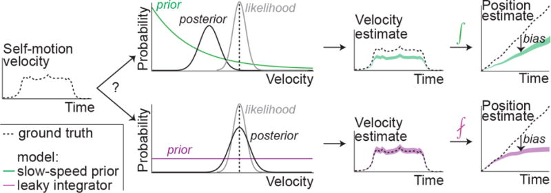
Subjects combine noisy sensory evidence from optic flow with prior expectations about self-motion speed to perform probabilistic inference over their movement velocity. The resulting noisy velocity estimates are integrated to generate beliefs about one’s position. Bias in position estimation might come about from two extreme scenarios. Slow-speed prior (green): A velocity prior that favors slower speeds coupled with perfect integration. Leaky integration (purple): A uniform prior over velocity coupled with leaky integration. For simplicity, this schematic shows the one-dimensional case. For general planar motion, both linear and angular velocity must be inferred and integrated to update position in two dimensions.

Although both the slow-speed and the leaky integration models can lead to overshooting, they attribute the bias to two very different sources – velocity underestimation or leaky dynamics. For uniform motion in one dimension, this difference can be readily detected by observing how the subject’s bias scales with distance: the bias due to a slow-speed prior will scale linearly, whereas leaky integration produces a sub-linear scaling ultimately leading to saturating estimates of position. However, when velocity changes over time, distinguishing the models requires analyzing the subject’s entire movement history rather than just comparing the pattern of bias in the stopping position. This framework allows us to incorporate measurements of the subject’s time-varying velocities to fit and distinguish the models.

Since the task was performed on a two-dimensional ground plane, subjects had to infer and integrate two components of their velocity (linear and angular). We assumed the two velocity components were integrated by separate integrators with possibly different time constants (Methods – Equation 2). Consequently, both models had four free parameters (see Methods): two likelihood widths to represent uncertainties in linear and angular velocity, and either two exponents to represent priors for those same components (for the slow-speed prior model) or two time constants to represent rates of leak in integrating them (for the leaky integrator model). Additionally, we fit a two-parameter null model that attributed subjects’ movements entirely to random variability, as well as a full model with six-parameters that featured both exponential priors and leaky integrators.

Model fitting and comparison

For each subject, we fit the models using the sequences of velocities along each trajectory. The models infer and integrate these velocity inputs and, depending on their parameters, generate specific trajectory estimates. Trajectories of different models correspond to the subject’s believed (rather than actual) positions during the trial. Our probabilistic framework assumes that subjects maintain estimates of both the mean and the uncertainty about their location, and steer to the target to achieve the greatest possible reward. We therefore fit the models to maximize the subject’s expected reward, defined as the overlap between the posterior distribution over their position and the target region at the end of each trial (Methods – Equation 3).

We found that the slow-speed prior model was about 1.35 times more likely per trial than the leaky integrator model for each individual subject. Multiplying this ratio over all trials, this means that speed misperception from a slow-speed prior is an overwhelmingly more likely explanation of subjects’ path integration biases than leaky integration (Fig S3A, mean (± standard error) log-likelihood ratio across subjects: 66.6 ± 18.2). Both models had substantially greater likelihoods than the null model, with larger improvements when biases were larger since the null model could not explain any bias (Fig S3B). Since the evidence supporting both the slow-speed prior and leaky integration models was correlated, we asked whether subjects’ behavior may have been influenced by both. To test this, we fit a model that incorporated both exponential prior and leaky integration. This full model was not much better at explaining subjects’ responses than the slow-speed prior model (Fig S3C). Moreover, for all subjects, the best-fit time constants of integration in the full model were much greater than the average trial duration (Fig S3D), implying that integration was nearly perfect in this model. Therefore, leaky integration could not explain any appreciable variability in the data in excess of what was already explained by the slow-speed prior.

We wanted to know why the slow-speed prior model performed better. A good behavioral model will believe that subjects should stop moving where they do stop. This means that the model’s beliefs about its position should be concentrated near the true target, even when the actual position has overshot. To evaluate this, we used the best-fit model parameters to reconstruct the subjects’ beliefs, given by the posterior distribution over their position throughout each trial as they steered towards the target. Belief trajectories implied by the two models during an example trial are shown in Figure 3A. Since the model has a cloud of uncertainty over position, the plots actually show this cloud of beliefs swept out over time. This is overlaid with the subject’s actual trajectory and the target position. On this trial, the beliefs implied by the slow-speed prior model (Fig 3A – left) terminated near the target, indicating that the subject strongly (and wrongly) believed he steered to the target location. On the other hand, the leaky integrator model believes it completely missed the target (Fig 3A – right), contradicting the basic premise that the subject is making a subjectively good decision.

Figure 3. Model comparison and validation.

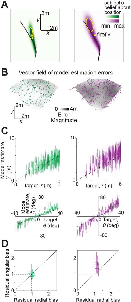
A. Posterior probability distribution over position implied by the best-fit slow-speed prior (left, green) and leaky integrator (right, purple) models, swept over time during an example trial for the subject with the largest bias. The distributions at different time points were rescaled to the same height, so these plots reflect this subject’s relative beliefs about his location across the duration of the trial. Target location (yellow dot) and the actual trajectory (black line) have been overlaid. Yellow ellipses depict an isoprobability contour (68% confidence interval) of the model posteriors over position at the end of the trial. B. Vector field of errors in the mean estimate of final position across trials, for the two models. Error vectors of both models were rescaled to minimize overlap. The spatial profiles of the error magnitude (distance between target and mean estimated final position) for the two models are shown by the grayscale background. C. Subject’s internal estimates of the radial distance $(\widehat{r},\mathit{left})$ and angle $(\widehat{\theta },\mathit{right})$, not to be confused with the subject’s actual response $\stackrel{\sim }{r}$ and $\stackrel{\sim }{\theta }$ in Fig 1E, are plotted against target distances and angles for the subject in (A,B). Internal estimates implied by the slow-speed prior and leaky integrator models are shown in green and purple respectively. Model estimates for each trial are shown as vertical bars centered on the mean, and ±1 standard deviation in length. D. Bias in model estimates (termed ‘residual bias’) of radial distance and angle for the two models, obtained by cross-validation (Methods). Error bars denote ±1 standard error of the mean obtained via bootstrapping. Dashed lines indicate unbiased radial or angular position estimates. Solid diagonal line has unit slope. See also Figure S3.

This difference between the models’ estimates of the final position was consistent across trials, as revealed by the much greater estimation error magnitudes for the leaky integrator model (Fig 3B – grey level). Moreover, unlike the slow-speed prior model, the vector field of errors in the estimates generated by the leaky integrator model was non-random (Fig 3B – arrows), betraying this model’s inability to fully account for the subject’s systematic errors. Note that the above model estimates are meant to reflect subjects’ internal beliefs about their position (which should be nearly unbiased) rather than their actual positions (which we know are biased). So the near-zero estimation error magnitude of the slow-speed prior model (Fig 3B) suggests that this model is almost entirely able to explain away the subject’s bias.

To assess the difference in the quality of fits of the two models, we compared the final position estimates generated by each of the two models against the target position (Fig 3C). This comparison is similar to the one used to evaluate subjects’ responses (Fig 1E), except that we now replace the subject’s actual position with the model estimates. We emphasize that we are modeling the subject’s internal estimates, not predicting their external response. Therefore, the quality of the model estimates should be assessed by comparing against the unit slope, not by comparing with Fig. 1E. For the example subject shown in Fig 3C, it can be readily seen that the estimates of the slow-speed prior model were in reasonably good agreement with target distances and angles. However, estimates generated by the leaky integrator model were still biased, and those biases were particularly large for nearby targets. Intuitively, this is because nearby targets only require short integrations, so the leak does not have time to take effect. Consequently, the leaky integrator model is objectively accurate at short times, and thus cannot account for the subjective biases in those trials, leading to a relatively poor fit. On the other hand, the slow-speed prior model attributes path integration bias to velocity underestimation, a bias which persists at all times and thus generalizes well across trials.

We quantified the goodness-of-fit of the models by computing residual biases in the model estimates of radial distance and angle using a four-fold cross-validation procedure (Methods). These residual biases were not significantly different from unity across subjects for the slow-speed prior model (mean ± sem residual radial bias=1.03 ± 0.04, p=0.27, t-test; residual angular bias=1.01 ± 0.1, p=0.36). On the other hand, residual biases of the leaky integrator model were significantly greater than unity (residual radial bias=1.09 ± 0.06, p=3.2×10⁻², residual angular bias=1.31 ± 0.14, p=3.4×10⁻³). Therefore, the slow-speed prior model provided a much better account of subjects’ biases (Fig 3D).

Recent studies on path integration have modeled leak using space constants instead of time constants, so that the integration dynamics are only active during movement. We formulated a variation of the model based on space constants (Methods) and found that it still performed worse in predicting subjects’ responses than the slow-speed prior model (Fig S3E). This is not surprising because spatial leak suffers from the same problem responsible for the relatively poor performance of the model with temporal leak. Finally, to verify consistency with the family of Bayesian models previously used in psychophysics, we considered other parameterizations of the slow-speed prior and leaky integrator models that incorporate a Gaussian prior (Hürlimann et al., 2002) or a log-normal likelihood (Jürgens and Becker, 2006; Stocker and Simoncelli, 2006), and we fit each alternative (Methods). On average, the slow-speed prior model continued to outperform the leaky integrator model in all cases (Fig S3F), indicating that our conclusions are robust to the specific choices of shapes of the prior and likelihood.

Test of model predictions

The likelihood comparison above clearly favors attributing the path integration bias to a slow-speed prior over leaky integration of velocity estimates. This makes new predictions, which we tested experimentally by manipulating parameters of the task. One manipulation involved changing the reliability of optic flow by varying the density of the ground plane elements between two possible values (sparse and dense). A hallmark of Bayesian inference is that, for unimodal non-uniform priors and symmetric likelihood functions, the bias increases for less reliable observations. Therefore, if subjects had a slow-speed prior, sparse optic flow would increase how much they underestimate their velocity, leading to a larger bias (Fig 4A). However, if the prior is uniform, the density of optic flow would merely affect subjects’ uncertainty about their speeds while the instantaneous optic flow estimates themselves would still be unbiased under both conditions. The leaky integrator model thus predicts that changing the texture density would leave position bias unaffected.

Figure 4. Test of model predictions.

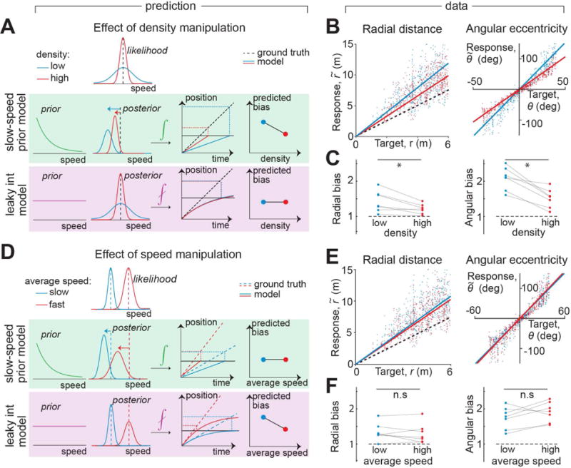
A. Reliability of optic flow was manipulated by altering the density of ground plane elements. Decreasing the density will increase subjects’ bias only if they have a slow-speed prior. B. Scatter plots showing the effect of density on radial and angular bias of one subject. Dashed line represents unity slope (unbiased performance) and solid lines represent slopes of regression fits. Trials are colored according to density – red: high density trials, blue: low density trials. C. Effect of density manipulation on radial (left) and angular (right) biases of individual subjects. Asterisks denote significant difference between means (see text). D. Subjects’ speed limit was manipulated by altering the gain of the joystick. The leaky integrator model predicts that subjects’ biases will be reduced in the high-speed condition. E. Scatter plots showing the effect of speed on distance and angle bias of one subject. Trials are colored according to speed – red: high speed trials, blue: low speed trials. F. Speed manipulation does not affect subjects’ biases in a systematic way. n.s. stands for not significant (see text). See also Figure S4.

The performance of an example subject is shown in Figure 4B. Sparsifying optic flow had a detrimental effect on behavior as indicated by a steeper relationship between true and perceived distance moved as well as angle rotated. As before, we quantified the bias as the slope of this regression and found similar effects across subjects (Fig 4C, Fig S4A). Consistent with the prediction of the slow-speed prior model, decreasing the density lead to a significantly greater bias both in distance moved (mean ± sem radial bias, Γ_r – high density: 1.27 ± 0.1; low density: 1.46 ± 0.1; p =2.5× 10⁻², paired t-test) and in angle rotated (mean angular bias, Γ_θ – high density: 1.58 ± 0.1; low density: 2.13 ± 0.1; p= 9.1×10⁻⁴).

In a second manipulation, we imposed two different speed limits (slow and fast) on different trials, which we implemented by randomly switching the gain by which the joystick controlled velocity. To avoid inducing different effects on biases in distance and angle, both linear and angular velocities were scaled by the same gain factor (Methods). Since the leaky integrator model incorporates a uniform prior, subjects’ estimates of speeds will always be unbiased in this model. However, a fundamental feature of this model is that the integration error accumulates over time, so lowering the speed limit should lead to a larger positional bias due to increased travel time (Fig 4D). On the other hand, for a Gaussian likelihood whose variance scales linearly with speed, an exponential slow-speed prior predicts that the velocity would be underestimated by the same multiplicative factor at all velocities. Therefore, the slow-speed prior model predicts that subjects will accurately perceive the relative change in their speeds and thus be biased to the same extent under both conditions. Note that this latter prediction strictly holds only for model parametrizations that produce a multiplicative bias in velocity estimates, and may not be applicable to alternative formulations of the model. However, the prediction of the leaky-integrator model’s speed dependence does not depend on the form of the velocity likelihood, and can therefore be unambiguously tested.

We analysed subjects’ biases and found that their performance was, on average, unaffected by the speed manipulation (Fig 4E-F, Fig S4B) both for distance (Γ_r – high speed: 1.33 ± 0.1; low speed: 1.38 ± 0.1; p=0.59, paired t-test) as well as angle (Γ_θ: high speed, 1.92 ± 0.1; low speed, 1.72 ± 0.1; p=0.15). This result is consistent with our preliminary observation of a velocity-independent distance bias (Fig S1C). This once again argues against the leaky-integrator model and favors, in particular, a slow-speed prior model that can induce multiplicative biases in velocity estimates.

Distance-dependent bias reversal

Since subjects compute their position by integrating noisy velocity estimates, their position estimates are uncertain. When traveling modest distances, such as those tested in the above experiments, the integrated uncertainty in position is relatively small. Although we took this uncertainty into account, we could qualitatively explain overshooting solely in terms of a bias in the subject’s mean position estimates resulting from integrating biased velocity estimates. In this section, we show that when path integrating over larger distances, the influence of position uncertainty can produce a reversal in the pattern of bias — from overshooting to undershooting — and we provide experimental evidence for this phenomenon.

Recall that the proposed framework assumes that subjects incorporate their knowledge of position uncertainty by tracking the expected reward of stopping at a given location. When this expected reward reaches its maximum, they stop moving. At any given moment during the trial, the expected reward is given by the overlap of the probability distribution over their position with the target. Let us examine how it should change as a function of their position, by considering uniform motion in one dimension for clarity. Subjects integrate both the mean (signal) and random fluctuations (“noise”) in their velocity estimates. If integration is leak-free, then their uncertainty in position would gradually keep building up over time (Methods – Equation 4). The rate at which position uncertainty builds up depends on the nature of sensory noise (independent or temporally correlated) as well as ability to represent and integrate large uncertainties. In principle, drift-diffusion models can be used to model noisy integration (Simen et al., 2011; Thurley, 2016). However, constructing such mechanistic models would entail making uninformed assumptions about the noise process. Here, rather than positing a particular mechanism, we choose a phenomenological model for position uncertainty, assuming that the standard deviation σ of the position distribution grows as a power-law function of time t, as σ (t) ∝ t^λ. For uniform motion, this can also be expressed as a distance-dependent scaling of the width with the same power-law exponent so that σ (r) ∝ r^λ for distance r (Fig 5A). A scaling exponent of λ = 0.5 (Wiener process) would result from integrating velocity estimates with independent Gaussian noise. Other types of noise may yield smaller (sub-diffusion) or larger (super-diffusion) exponents, depending on whether variance in the position estimate (σ²) scales faster or slower than the mean.

Figure 5. Model explains bias reversal with distance.

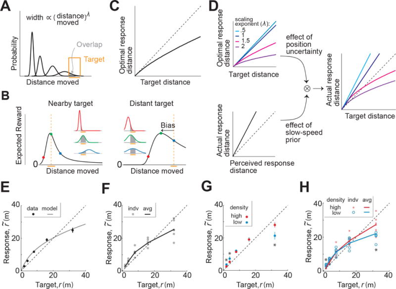
A. The width of the subjects’ probability distribution over their position (black) is modeled as a power law with exponent λ. The overlap (grey shade) of the probability distribution with the target (orange) corresponds to the subjects’ expected reward. B. Evolution of subjects’ expected reward when steering to a nearby (left) and distant (right) target for λ = 1.5 and proportionality constant equal to one. Insets show probability distributions over position at three different locations indicated by solid circles of the corresponding color on the reward curve. The peaks of the reward curves correspond to the optimal response distance. Orange bars denote the width of the target and dashed vertical lines the target center. C. The optimal response distance as a function of target distance, for the above case. D. The effect of position uncertainty (top) and the effect of slow-speed prior (bottom) combine to determine the model prediction for path integration bias, shown for various values of the power-law exponent (right). The interaction scales the optimal response distance by the slope Γ of the relation between actual and perceived distance moved. E. Mean net distance moved by one subject in response to targets at five different distances. Grey solid line corresponds to the best-fit model. F. Grey circles denote mean responses of individual subjects. Black line corresponds to the subject-averaged response. G. Mean response of one subject under conditions of low-density (blue) and high-density (red) optic flow. Asterisks denote a significant difference between mean responses under the two conditions (2m: p=0.029, 4m: p=0.007, 32m: p=4.1×10⁻⁴, paired t-test). H. Mean responses of individual subjects under the two conditions. Asterisks denote a significant difference between mean responses (across subjects) under the two conditions (2m: p=0.035, 32m: p=0.013, paired t-test). Solid lines correspond to subject-averaged response. (C-H) Black dashed lines have unit slope; (E, G) Error bars denote standard error of mean across trials. See also Figure S5.

We analysed how the expected reward should qualitatively depend on distance for a range of exponents. Intuitively, one would expect it to be greatest when the probability distribution over position is centered on the target. However, this is not always true. Figure 5B shows how the expected reward evolves with distance for near and far targets for one example case (λ = 1.5). When steering to nearby targets, the built up uncertainty is relatively small so the expected reward is indeed greatest when the mean of the distribution over distance moved roughly matches the target distance. For faraway targets however, the expected reward actually peaks before reaching the target. This happens because, if the subject moves beyond that optimal distance, the probability distribution over their position becomes so wide that its overlap with the target begins to decrease. Therefore, when steering towards sufficiently distant targets, an ideal observer should stop short of the target (Fig 5C).

The precise extent of undershooting depends on the noise process, with larger exponents producing greater undershooting due to a faster build-up in uncertainty (Fig 5D – top left). Furthermore, for exponents larger than one, the tendency to undershoot grows stronger with distance. Note that the degree of undershooting does not depend on the uncertainty in estimating the target position, but rather on the change in uncertainty over distance. Any uncertainty about the target would reduce the magnitude of expected reward but not the optimal distance at which maximum reward is achieved. Thus, potentially, large biases in path integration can stem solely from a subject hedging their bets against increasingly uncertain position estimates — even when those estimates are unbiased. We have already demonstrated that velocity, and consequently the distance moved, is likely underestimated due to a slow-speed prior (Fig 5D – bottom left). The two factors will have opposing effects on bias, with potentially different spatial dependences: whereas the slow-speed prior causes overshooting through a perceptual bias that scales linearly with distance, growing uncertainty does not alter the perceptual bias but generates an increasing tendency for responses to undershoot. This undershooting can increase linearly or supra-linearly depending on whether uncertainty scales slower (λ < 1) or faster (λ > 1) than Weber’s law. The combined effect of the two factors is shown in Figure 5D (right). For sub-Weber-law scaling in uncertainty, bias will increase linearly with distance, consistently producing either overshooting or undershooting depending on the relative strength of the two effects. For scaling exponents larger than one, the different spatial scaling from the slow-speed prior and from growing positional uncertainty — leads to a rather surprising prediction: when position uncertainty grows faster than the mean, bias in the subjects’ responses should gradually reverse from overshooting to undershooting when navigating to increasingly distant targets.

The above prediction also holds for motion in two dimensions. In this case, both linear and angular components of motion are subject to the effects of growing uncertainty, and may eventually lead to undershooting both in radial as well as angular responses. To test whether there is such a bias reversal, we conducted an additional experiment in which we asked subjects to steer to targets that were much further away. Target locations were discretized and their distances were varied on a logarithmic scale (Methods). Since the limited viewing angle in our set up restricted the angular eccentricity of the targets, we did not test for bias reversal in the angular domain. Similar to our original experiment, subjects continued to exhibit a significant angular bias (Γ_θ = 2.32 ± 0.6, p = 1.6 × 10⁻⁴, t-test, Fig S5A), turning much more than required.

On the other hand, the pattern of radial bias was strikingly consistent with our prediction. Figure 5E shows how the radial distance of an example subject scaled with target distance in this task. The subject exhibited overshooting in trials with nearby targets ([2, 4, 8, 16] m), as was observed in the original task, but this pattern of bias was replaced by significant undershooting for the farthest targets (32 m). Note that when steering to distant targets, the effect of the slow-speed prior would still persist but its effect is outweighed by that of increasing positional uncertainty. To quantify the relative strength of the two effects, we simultaneously fit a multiplicative constant Γ and exponent λ to the subject’s data (Methods – Equation 5). The multiplicative constant captures the linear effect of velocity underestimation that causes overshooting, while the exponent reveals the rate of scaling of uncertainty with distance that causes undershooting to faraway targets. Both parameters must be greater than unity in order to produce a reversal from overshooting to undershooting. This was indeed the case for this subject (Fig 5E – grey curve; Γ = 2.2, λ = 2.4). A similar pattern of bias reversal was observed across subjects (Fig S5B; Γ = 1.5 ± 0.2, p=3.6×10⁻⁵, t-test; λ = 1.8 ± 0.4, p=8×10⁻⁵) and can be noticed in the subject-averaged responses (Fig 5F). The supra-Weber-law scaling in subjects’ uncertainty can also be explicitly seen in the manner by which standard deviations in response scaled with the mean distance moved (Fig S5C).

The undershooting observed for distant targets could simply have been due to motor fatigue. To test whether the bias was influenced by sensory uncertainty, we re-analysed our data by dividing the trials into two groups based on the density of optic flow cues. If sensory uncertainty contributes to undershooting, decreasing the reliability of sensory cues should cause greater undershooting. The behavior of an example subject shown in Figure 5G confirms this assertion. When steering to the farthest target, this subject covered significantly less distance when the density of optic flow was reduced. Note that for nearby targets, the effect is reversed because the influence of the slow-speed prior is stronger than that of position uncertainty. These effects of density manipulation were observed across subjects (Fig 5H; Fig S5D), suggesting that subjects’ bias is likely not due to fatigue, but rather governed by sensory uncertainty.

The bias-reversal reported here should not be confused with an experience-based regression effect in which subjects’ responses are biased towards the mean stimulus (Jazayeri and Shadlen, 2010; Petzschner and Glasauer, 2011). Specifically, due to noise in the measurement of the target location, subjects’ perceptual estimates of that location may be biased towards the mean of the distribution of targets across trials; in turn, this could manifest in path integration behavior that is similarly biased. However, the pattern of bias shown in Figure 5 was present from the beginning of the experiment (Fig S5E), suggesting that this bias is not likely due to effects of adaptation. Furthermore, to ensure that manipulating ground-plane density does not influence judgement of target location, we conducted a separate experiment in which we manipulated ground-plane density only after the target was turned off so that it selectively affects reliability of optic flow. Once again, we observed that bias-reversal was sensitive to this manipulation (Fig S5F, G) implying that it is induced by the process of path integration, rather than a bias in target perception. While regression to the mean may still play a role in this task, our results suggest that prior expectations about self-motion velocity, and uncertainty in position due to accumulated uncertainty about optic flow, have a dominant influence.

DISCUSSION

We have presented a unified framework that combines Bayesian inference, evidence integration, and the principle of utility maximization to explain human behavior in a naturalistic navigation task. This framework yields a parsimonious account of bias in visually-guided path integration in which bias stems from prior expectations and sensory noise associated with self-motion. Our claim is based on four primary findings. First, when navigating modest distances using optic flow, humans overshoot the goal location, implying that they underestimated both their net translation and rotation. Second, analysis of subjects’ movement trajectories using a dynamic observer model revealed that their bias was more likely to originate from a slow-speed prior rather than forgetful integration of self-motion. Third, experimental outcomes of manipulating the reliability of self-motion cues and speed confirmed the predictions of the slow-speed prior model. Finally, when navigating long distances, the model predicts a possible reversal in the direction of bias due to the growing influence of uncertainty on the expected reward, a phenomenon that was confirmed experimentally.

In order to study visual path integration, we used virtual reality so that vestibular and proprioceptive inputs were no longer relevant for the task. Specifically, subjects used a joystick to steer to a cued target location based solely on optic flow. To perform accurately on this task, participants had to determine the location of the target, remember that location, and integrate their own movements until they reached that location. Each of those steps is a potential source of behavioral errors.

There are several reasons why systematic errors seen in our data cannot be attributed to biased perception of the initial target location. First, we used stereoscopic stimuli to generate an immersive virtual environment with depth cues that facilitate judgement of target distances, at least for short distances. Second, judging target angles is more straightforward and does not require depth cues, yet subjects exhibited a large angular bias in the task. Notably, introducing angular landmarks in the virtual environment abolished this angular bias. The landmarks themselves were uninformative about target angles, but helped obviate the need to integrate angular velocity by providing a direct estimate of the subject’s orientation in the virtual environment. Thus the large angular biases seen in the absence of landmarks must be related to the perception of optic flow cues. Finally, and perhaps most importantly, manipulating the density of the ground plane significantly altered subjects’ biases at all distance scales. This effect persisted even when we confined the above manipulation to the period of movement, leaving target distance estimation relatively intact. Therefore, the behavioral bias seen in our task likely reflects error in estimating one’s own position, rather than difficulties associated with estimating the target location.

Relation to past experiments

Past studies on visual path integration employed visually simulated motion along a straight line or along predetermined curvilinear trajectories. In contrast, our experimental task allowed subjects to actively steer using two degrees of freedom allowing for precise control of their self-motion velocity at all times, as would be the case during natural foraging. This design was motivated by the need to engage neural mechanisms and computations that likely underlie path integration in the real world. Yet, our results regarding biases are qualitatively similar to those of previous studies, even though those studies tested motion along a one dimensional hallway. Specifically, studies that tested visual path integration over short distances found that subjects overshoot the target (Frenz and Lappe, 2005; McManus et al., 2017) while studies that used long-range targets found the opposite (Brossard et al., 2016; Lappe et al., 2007; Redlick et al., 2001). A noteworthy departure from past studies was observed in the manner by which variability of our subjects’ responses scaled with distance. Like sensory perception, odometric ability has been shown to follow Weber’s law in humans (Durgin et al., 2009; Petzschner and Glasauer, 2011) and invertebrates (Cheng et al., 1999, 2006). In contrast, we observed supra-Weber-law scaling. Given that the overall magnitude of response variability was also larger in our study, we suspect that the use of sparse optic flow in our experiments – needed to probe the internal model of subjects’ self-motion velocity – underlies the above discrepancy. If this is the case, then it suggests that Weber’s law might break down in the regime of high uncertainty.

Relation to past models

To explain our subjects’ behavior, we tested two different instantiations of a dynamic Bayesian observer model and found that bias in path integration appears to stem mainly from a slow-speed prior that causes subjects to underestimate their velocity. Unlike a prior over retinal speed (Hürlimann et al., 2002; Sotiropoulos et al., 2014; Stocker and Simoncelli, 2006; Weiss et al., 2002), the prior in our Bayesian model corresponds to subjects’ prior expectation of their self-motion velocity. Nonetheless, the latter might be inherited from low-level visual sensory priors that govern human perception of local image velocities. Alternatively, the prior over self-motion velocity could reflect the statistics of sensory inputs experienced during natural self-motion, which is known to be biased towards slower velocities (Carriot et al., 2014). In this case, one would expect the prior to be shared across all modalities. Our data qualitatively agrees with this view for the prior over angular velocities, since angular bias persisted when estimates were based on efference copy alone, although the variability was prohibitively large to allow for a proper quantitative assessment (Fig S1B). Regardless of its specific origins, this work demonstrates that sensory priors can have tangible consequences for complex dynamic behaviors such as path integration, well beyond the realm of traditional binary decision-making tasks. Although we focused on visual self-motion, this model is also applicable to other modalities. Availability of additional modalities should diminish the effect of the prior leading to reduced bias. Such a reduction has in fact been observed when path integrating using multimodal cues (Bakker et al., 1999; Becker et al., 2002; Sun et al., 2004).

While the slow-speed prior can explain why subjects would travel beyond the goal, it cannot account for undershooting reported in previous studies that used distant goals (Brossard et al., 2016; Lappe et al., 2007; Redlick et al., 2001). However, analysis of our model revealed that when path integrating over longer distances, the effect of growing uncertainty can eventually override the effect of perceptual bias induced by prior expectations and cause undershooting in subjects’ responses. This is a spatial analog of a model that explains early abandonment on a waiting task as a rational response to increasing uncertainty about the next reward (McGuire and Kable, 2013). We tested this prediction and found that the pattern of bias changed from overshooting to undershooting, when navigating to increasingly distant targets. This phenomenon of bias-reversal is also discernable in the results of previous visual (Brossard et al., 2016; Lappe et al., 2007; Redlick et al., 2001) and non-visual (Bergmann et al., 2011; Lappe and Frenz, 2009) path integration studies. Traditional leaky integration models cannot explain why subjects would undershoot. To account for undershooting, such models have had to be modified to update distance-to-target rather than distance moved (Frenz and Lappe, 2005). However, such a change of variable neither explains why subjects overshoot to relatively nearby goals, nor why the degree of undershooting is sensitive to the reliability of optic flow. Here we show that a distance-dependent reversal in the response bias naturally emerges when performing probabilistic inference over position under the influence of a slow-speed prior, to maximize expected reward. Although velocity estimates are more reliable at smaller speeds, moving slowly would entail integrating over longer times and consequently, subjects would not benefit from such a strategy (Fig 4F). In fact, longer integration times would result in an even greater accumulated uncertainty due to the supra-Weber-law scaling effect (Fig S5C). Perhaps this explains why subjects tended to travel close to the speed-limit in our task (Fig S1C).

Recent models based on iterative Bayesian estimation suggest that subjects may exploit trial-history to update an explicit prior over net distances and angles turned (Petzschner and Glasauer, 2011; Prsa et al., 2015). While such models can explain responses that exhibit a regression towards the mean of previously experienced stimuli, they cannot account for the unidirectional response bias observed in many studies, including our own (Fig 1E). Moreover, such models have limited potential for explaining systematic biases seen in the first few trials of the experiment when the subjects have not yet accurately learned the environmental statistics.

Other models attribute bias in path integration primarily to either a path-dependent (Bergmann et al., 2011; Brossard et al., 2016; Lappe et al., 2007, 2011) or temporal (Mittelstaedt and Glasauer, 1991; Mittelstaedt and Mittelstaedt, 2001; Vickerstaff and Di Paolo, 2005) decay in integrating self-motion. However, leaky integration cannot explain the effect of reliability of optic flow cues reported here. Moreover, it is worth noting that, in addition to the leak factor, a recent model of “leaky-integration” incorporated a gain factor that rescaled subjects’ displacement in each step. The best-fit gain factors were generally less than unity (Bergmann et al., 2011; Brossard et al., 2016; Lappe et al., 2007, 2011) which essentially amounts to velocity underestimation. Coupled with small leak rates (~0.01–0.02m^-1) found in those studies, it is clear that the performance of that model for short-range targets is in fact dominated by velocity underestimation.

Although the precise neural circuit underlying path integration has not been worked out, there is physiological evidence for near-perfect integration of visual motion cues by neurons in macaques (Huk and Shadlen, 2005; Kiani et al., 2008) suggesting that our model is neurally plausible. Our work is also supported by recent studies showing lossless evidence accumulation of temporally disjoint sensory inputs in rats (Brunton et al., 2013; Raposo et al., 2014), humans (Brunton et al., 2013; Kiani et al., 2013), and monkeys (Huk and Shadlen, 2005; Kiani et al., 2008) performing binary-decision tasks. Subjects may benefit from imperfect integration when the statistical structure of sensory inputs is unpredictable (Carland et al., 2016; Glaze et al., 2015) or when signal strength fluctuates wildly (Ossmy et al., 2013; Veliz-Cuba et al., 2016). However, when sensory dynamics are known a priori or are predictable from physical laws, it makes sense that behavior is limited by sensory inputs, rather than leaky integration. One limitation of this work is that it is based solely on the principle of probabilistic perceptual inference and ignores the costs incurred in performing actions. Since navigation is effortful, future extensions should test whether the subjects also optimize their actions at finer timescales to minimize the total cost during goal-oriented navigation.

Toward understanding the neural basis

Disentangling the neural representation of sensory inputs from internal beliefs is notoriously difficult. Binary-decision tasks and other paradigms measuring discrete responses are ill-suited for this purpose, as behavioral readouts are often sparse in time and may conflate beliefs states and actions. The task and the modeling approach used in this study offer an ideal setting to overcome such limitations to investigate ‘dynamic belief state representations’ (Lee et al., 2014) in a widely studied neural circuit. Specifically, theoretical models suggest that grid cells may be involved in path integration (Burak and Fiete, 2009; Giocomo et al., 2011), yet experimental evidence remains indirect (Chen et al., 2015; Gil et al., 2018) and controversial (Bjerknes et al., 2018). By properly modeling the beliefs of animals trained to path integrate, one can distinguish the spatiotemporal dynamics of their belief states from actual states (e.g. Fig 3A – left), and then look for the neural correlates of those states in the grid cell network.

Beyond characterizing neural representations, the approach outlined here would also allow one to directly test the optimality of the underlying neural computations. For instance, brain areas encoding self-motion velocity have recently been identified in rodents (Kropff et al., 2015; Whitlock et al., 2012; Wilber et al., 2017) and primates (Avila et al., 2017). By simultaneously recording the activity of areas representing velocity and internal estimates of position, one can test whether brain-wide neural circuits can optimally integrate dynamic, non-stationary sensory inputs, which would help unravel how the brain works in the real world.

STAR METHODS

Contact for Reagent and Resource Sharing

Further information and requests for resources and reagents should be directed to and will be fulfilled by the Lead Contact, Kaushik Lakshminarasimhan (jklakshm@bcm.edu).

Experimental Model and Subject Details

Nineteen human subjects (Nine Male, Ten Female; all adults in the age group 18-32) participated in the experiments. With the exception of subjects s4 and s5 (Figures 1, 3, and 4), all subjects were unaware of the purpose of the study. Experiments were first performed in the above two subjects before testing others. All experimental procedures were approved by the Institutional Review Board at Baylor College of Medicine and all subjects signed an approved consent form.

Method Details

Behavioral Task

Subjects used an analog joystick with two degrees of freedom and a circular displacement boundary to control their linear and angular speeds in a virtual environment. This virtual world comprised a ground plane whose textural elements had limited lifetime (~250ms) to avoid serving as landmarks. The ground plane was circular with a radius of 70m (near and far clipping planes at 5cm and 4000cm respectively), with the subject positioned at its center at the beginning of each trial. Each texture element was an isosceles triangle (base × height: 8.5 × 18.5 cm) that was randomly repositioned and reoriented at the end of its lifetime, making it impossible to use as a landmark. The stimulus was rendered as a red-green anaglyph and projected onto a large rectangular screen (width × height: 149 × 127 cm) positioned 67.5cm in front of the subject’s eyes. Subjects wore goggles fitted with Kodak Wratten filters (red #29 and green #61) to view the stimulus. The binocular crosstalk for the green and red channels was 1.7% and 2.3% respectively. Subjects pressed a button on the joystick to initiate each trial, and the task was to steer to a random target location that was cued briefly at the beginning of the trial (Fig 1A). The target, a circle of radius 20cm whose luminance was matched to the texture elements, blinked at 5Hz and appeared at a random location between θ = ±42.5° of visual angle at a distance of r = 0.7 – 6m relative to where the subject was stationed at the beginning of the trial. After one second, the target disappeared, which was a cue for the subject to start steering, and the joystick controller was activated.

Of the nineteen subjects, seven subjects performed a total of 2000 trials equally spread across eight sessions. Prior to the first session, all subjects were asked to perform around ten practice trials in which they steered to a visible target to familiarize themselves with joystick movements and the task structure. In four of the sessions (two of which contained angular landmarks in the form of a panoramic mountainous background), the maximum linear and angular speeds were fixed to ν_max = 2ms⁻¹ and ω_max = 90°/s respectively, with the floor density also held constant at ρ = 2.5 elements/m². In the remaining four sessions, trials with two different speed limits (ν_max = 2ms⁻¹ and ω_max = 90°/s; ν_max = 4ms⁻¹ and ω_max = 180°/s) and two floor densities (ρ = 0.1 elements/m² and ρ = 2.5 elements/m²) were randomly interleaved. Six of the seven subjects participated in two additional experimental sessions (250 trials each). The first of these additional experiments was similar to the original experiment except that half the trials contained no optic flow cues, so subjects had to steer in complete darkness. In the second additional experiment, as before, subjects pressed a button on the joystick to initiate each trial. Targets appeared briefly at random locations sampled from a distribution identical to the original experiment. However, rather than actively steering to the target, they were passively transported along trajectories that took them through the target at one of two possible linear speeds (ν = 2ms⁻¹ or 4ms⁻¹). Since trajectories necessarily passed through the target and the velocity was held constant throughout the trial, the angular velocity on each trial was constrained by the location of the target. Subjects were instructed to press the button when they believed they had reached the target. Therefore, in this experiment, subjects used the joystick only to initiate trials and register their responses.

Furthermore, six subjects (five of whom did not participate in any of the above studies) were tested on an extended version of the original task wherein the targets were presented at distances of up to 32m. Due to the longer range of distances used in this version, the target radius was increased from 20cm to 75cm to ensure clear visibility. As before, subjects had to steer to a target location that was cued briefly for a period of 1 second at the beginning of the trial. However in this experiment, target locations were discretized to five possible distances (r = [2, 4, 8, 16, 32] m) and five possible angular eccentricities (θ = [0°, ±15°, ±30°]) resulting in a total of 25 unique target locations. Subjects performed ten randomized repetitions of each location yielding a total of 250 trials. Trials with two different floor densities (ρ = 0.1 elements/m² and ρ = 2.5 elements/m²) were randomly interleaved. Finally, seven more subjects (none of whom participated in any of the above studies) performed a slight variation of this extended task in which we manipulated the density only after the target was turned off. This ensured that the manipulation selectively affected the reliability of optic flow, but not the perception of target positions.

Stimulus and Data acquisition

All stimuli were generated and rendered using C++ Open Graphics Library (OpenGL) by continuously repositioning the camera based on joystick inputs to update the visual scene at 60 Hz. The camera was positioned at a height of 1m above the ground plane. Spike2 software (Cambridge Electronic Design Ltd.) was used to record and store the subject’s linear and angular velocities, target locations, and all event markers for offline analysis at a sampling rate of $833\frac{1}{3}\text{Hz}$.

Dynamic Bayesian observer model

To account for the pattern of behavioral results, we considered an observer model comprised of a Bayesian estimator that used noisy measurements m_ν and m_ω to decode linear and angular self-motion velocities ν and 0, which were then temporally integrated to dynamically update the subject’s position. We parameterized the model by making the following three assumptions: First, we chose an exponential function to describe the priors over both linear and angular velocities: $p(\nu )=e^{a_{\nu }\left|\nu \right|}$ and $p(\omega )=e^{a_{\omega }\left|\omega \right|}$. Second, likelihood functions p(m_ν|ν) and p(m_ω|ω) were assumed to be Gaussian, centered around the respective measurements m_ν and m_ω, with variances proportional to the magnitude of the measurement: Var(m_ν) = b_ν |m_ν| and Var(m_ω) = b_ω|m_ω|. Under these conditions, it can be shown that the means and variances of the maximum a posteriori estimates $\widehat{\nu }$ and $\widehat{\omega }$ are given by (Stocker and Simoncelli, 2006):

$$\mathrm{E}[\widehat{\nu }|m_{\nu }]={\beta }_{\nu }{m}_{\nu };\mathrm{E}[\widehat{\omega }|m_{\omega }]={\beta }_{\omega }{m}_{\omega }$$ (1.1)

$$\text{Var}[\widehat{\nu }|m_{\nu }]\approx {\beta }_{\nu }^2\text{Var}(m_{\nu });\text{Var}[\widehat{\omega }|m_{\omega }]\approx {\beta }_{\omega }^2\text{Var}(m_{\omega })$$ (1.2)

where β_ν = 1 + a_νb_ν and β_ω = 1 + a_ωb_ω have a straight-forward interpretation in the form of multiplicative biases in the subjects’ estimates of their linear and angular speeds respectively. Note that a flat prior corresponds to an exponent of zero yielding an unbiased estimate, while negative/positive values of the exponents would result in under/overestimation of the speeds. The final assumption pertains to the nature of the integrator that computes position from speed. We assume that the integration process is governed by two independent leak time constants τ_d and τ_φ that specify the timescales of integration of estimated linear and angular speeds to compute distance d and heading φ respectively:

$$\dot{d}=-d(t)/{\tau }_d+\widehat{\nu }(t);\dot{\phi }=-\phi (t)/{\tau }_{\phi }+\widehat{\omega }(t)$$ (2.1)

The mean distance and heading at each time point can be determined by convolving the mean velocity estimates with an exponential kernel: $\mathrm{E}[\widehat{d}(t)]=e^{-t/{\tau }_d}\circ \mathrm{E}[\widehat{\nu }(t)]$ and $\mathrm{E}[\widehat{\phi }(t)]=e^{-t/{\tau }_{\phi }}\circ \mathrm{E}[\widehat{\omega }(t)]$ where the expectations are taken over the corresponding posterior probability distributions. Likewise, if noise in the velocity measurements is temporally uncorrelated, the variance of the distance and heading estimates can be expressed in terms of the variances of the velocity estimates as: $\text{Var}[\widehat{d}(t)]=e^{-t/{\tau }_d}\circ \text{Var}[\widehat{\nu }(t)]$ and $\text{Var}[\widehat{\phi }(t)]=e^{-t/{\tau }_{\phi }}\circ \text{Var}[\widehat{\omega }(t)]$. Thus, in this case, both mean and variance of the integrated estimates will share the same temporal dynamics. Note that the mean estimates $\mathrm{E}[\widehat{d}(t)]$ and $\mathrm{E}[\widehat{\phi }(t)]$ will be accurate in the limit of large time constants (perfect integration), but are misestimated if the time constants are comparable to travel time, T. Since the timecourse of distance and heading together determine position, it follows that the subjects’ mean estimates of their linear and angular coordinates $(\widehat{r}\text{and}\widehat{\theta })$ will also be different from their actual values (r and θ) when τ ≈ T.

We also analysed a variation of the leaky integration model in which the leak was implemented using space constants π_d and π_φ according to:

$$\dot{d}=-\widehat{\nu }(t)d(t)/{\pi }_d+\widehat{\nu }(t);\dot{\phi }=-\widehat{\omega }(t)\phi (t)/{\pi }_{\phi }+\widehat{\omega }(t)$$ (2.2)

Note that unlike the temporal leak model in Equation 2.1, this model only integrates when velocity is non-zero. Therefore, position is only updated during movement resulting in estimates that are robust in time. This version of the leaky-integrator model was used for Fig S3E.

Model fitting

In order to determine the key factor underlying subjects’ biases, we fit two different variants of the model: (i) A ‘slow-speed prior model’ (ℳ₁) in which the integration was assumed to be perfect (τ_d = τ_φ = ∞) and (ii) a ‘leaky integration model’ (ℳ₂) where the prior was held flat (a_ν = a_ω = 0). These models represent the two extreme scenarios in which bias in path integration is attributed exclusively to speed misperception and forgetful evidence accumulation, respectively. The models both had four parameters each: width parameters (b_ν and b_ω) of the two likelihood functions to represent how fast the respective widths scale with the magnitude of linear and angular velocity measurements, in addition to either two exponents (a_ν and a_ω) to represent priors in ℳ₁ or two time constants (τ_d and τ_φ) to represent the degree of leak in ℳ₂. Since subjects’ position estimates are probabilistic, we fit model parameters ψ by taking both mean and uncertainty of position into account; this was done by maximizing the expected reward, which is essentially the probability that the subjects believed themselves to be within the target at the end of each trial:

$${\mathcal{L}}_{\mathcal{M}}=\underset{\psi }{\arg max}{\displaystyle {\prod }_{i=1}^N{\displaystyle {\int }_{-\mathrm{\infty }}^{\mathrm{\infty }}P}\left({\mathbf{x}}^{(i)}|{\dot{x}}_{1,\dots ,T}^{(i)}\right){\mathrm{𝟙}}_Q(\mathbf{x})d\mathbf{x}}$$ (3)

where x is a vector that denotes position on the horizontal plane, $P({\mathbf{x}}^{(i)}|{\dot{x}}_{1,\dots ,T}^{(i)})$ is the probability distribution over the subject’s stopping position on the i^th trial conditioned on the path taken in that trial, T is the duration of that trial, 𝟙_Q(x) is the indicator function which is equal to 1 for all values of x that fall within the target Q and zero everywhere else, ℒ_ℳ denotes the likelihood of model ℳ with the best-fit parameters, and model parameters ψ ∋ {a_ν, a_ω, b_ν, b_ω} and {b_ν, b_ω, τ_d, τ_φ} for ℳ₁ and ℳ₂ respectively. We fit two more models in addition to the above: a ‘null’ model ℳ₀ that had only two free parameters – ψ ∋ {b_ν, b_ω} – essentially attributing the biases in subjects’ position estimates entirely to random variability in their self-motion speed estimates, and a ‘full’ model ℳ₁₂ in which all six model parameters were free such that ψ ∋ {a_ν, a_ω, b_ν, b_ω, τ_d, τ_φ}.

In addition to the above parametrization, we fit both the slow-speed and leaky-integrator models using three alternative parametrizations constructed by changing either the form of the prior, the form of the likelihood function, or both: (i) Gaussian prior and Gaussian likelihood, (ii) Exponential prior and log-normal likelihood, and (iii) Gaussian prior and log-normal likelihood. Each of the above parametrizations also had four free parameters (Fig S3F). Maximum a posteriori estimates $\widehat{\nu }$ and $\widehat{\omega }$ were computed numerically.

Modeling position uncertainty

Since position is estimated by integrating velocity, uncertainty in velocity estimates will accumulate over time, leading to growing uncertainty in position estimates. If integration is leaky, noise will only accumulate over the time constant of integration, causing position uncertainty to eventually asymptote to a fixed value. However, if the integration is perfect, noise will accumulate perpetually leading to uncertainty that grows with time. Let r(T) denote the subject’s one-dimensional position estimate at time T. If ν(t) denotes subject’s instantaneous velocity estimate, we have:

$$r(T)={\displaystyle {\int }_0^T\nu (t)dt}+{\displaystyle {\int }_0^T\eta (t)dt}$$ (4)

where η(t) represents a noise in the velocity estimate and the integral of this noise corresponds to a random walk. If noise has zero mean, the subject’s mean position estimate 〈r(T)〉 is not affected. However, the noise variance of position estimate σ = 〈(δr)²〉 will grow with time. For integration of temporally uncorrelated noise, the variance of position uncertainty is proportional to time T. We postulate that uncertainty in position, δr, will be proportional to T^λ for some exponent λ. Large exponents may occur due to temporal correlations, or computational constraints within the system. For the case of uniform motion, ν(t) = ν, the mean position estimate is $\langle r(T)\rangle =\langle {\displaystyle {\int }_0^T\nu dt}\rangle =\nu T$. Since mean position then scales linearly with time, position uncertainty can be expressed in terms of position as σ (r) = kr^λ for some proportionality constant k.

Fitting distance-dependent bias reversal

To simultaneously quantify the effects of position bias (due to velocity underestimation) and position uncertainty leading to a distance-dependent bias-reversal, we modeled the subject’s radial distance response as:

$${\widehat{r}}_i=\Gamma \underset{r_i}{\arg max}{\displaystyle \underset{-\mathrm{\infty }}{\overset{\mathrm{\infty }}{\int }}P(r_i|k,\gamma ){\mathrm{𝟙}}_Q(r)dr}$$ (5)

where ${\widehat{r}}_i$ is the model estimated radial distance on the i^th trial, $P(r_i|k,\lambda )~\mathcal{N}(r_i,k{r}_i^{\lambda })$ is the modeled probability distribution over the subject’s position, 𝟙_Q (r) is the indicator function which is equal to 1 for all values of within the target Q and zero otherwise, and Γ is a multiplicative constant that captures multiplicative bias in the subject’s mean position estimate. If the mean position is underestimated, the multiplicative bias should be greater than unity because the subject would respond by overshooting. The integral on the right-hand side represents the subject’s belief that he/she is on target, and captures the effect of position uncertainty, whereas the multiplicative constant captures the bias in mean position induced by prior expectations of self-motion velocity. For each subject, we fit the model parameters Γ, λ, and k by minimizing the squared-error between the radial distance of the model and the subject’s actual response across trials according to $\underset{\Gamma ,\lambda ,k}{\arg min}{\displaystyle {\sum }_{i=1}^N{({\widehat{r}}_i-r_i)}^2}$ where N is the total number of trials.

Quantification and Statistical Analysis

Customized MATLAB code was written to analyse data and to fit models. Depending on the quantity estimated, we report statistical dispersions either using 95% confidence interval, standard deviation, or standard error in the mean. The specific dispersion measure is identified in the portion of the text accompanying the estimates. For error bars in figures, we provide this information in the caption of the corresponding figure. We report exact p-values for all statistical tests, and describe the outcome as significant if p < 0.05. Model parameters were optimized using MATLAB’s fmincon function by constraining time constants and likelihood widths to be non-negative.

Estimation of Bias

Behavioral error on each trial was quantified by computing the difference between the subject’s response position and the corresponding target position to yield an error vector $\overrightarrow{e}$. Error magnitudes were computed as the Euclidean norm of the error vectors, and were convolved with a two-dimensional isotropic Gaussian kernel g(x, y) with width 50cm to yield smoothed error magnitudes e_s (x₀, y₀) = Σ_x,y g (x − x₀, y − y₀)e(x, y) for visualization in Figure 1D. To visualize spatial distribution of errors for the two models (Fig 3C), we replaced subject’s response position by the position estimates generated by the models. We regressed each subject’s response positions $(\stackrel{\sim }{r},\stackrel{\sim }{\theta })$ against target positions (r, θ) separately for the radial $(\stackrel{\sim }{r}\text{vs}r)$ and angular $(\stackrel{\sim }{\theta }\text{vs}\theta )$ co-ordinates, and the radial and angular multiplicative biases (Γ_r and Γ_θ) were quantified as the slope of the respective regressions (Fig 1E). Quantifying the biases in this polar representation of the positions allowed us to qualitatively relate them to perceptual biases in linear and angular speeds — quantities that the subjects controlled using the joystick. For each subject, we estimated the 95% confidence interval in the biases by bootstrapping (Fig 1F). We used a one-sample t-test to determine whether the mean multiplicative bias across subjects was significantly greater than unity (n=7).

Model comparison and validation

For each subject, we estimated the likelihoods of all four models – the slow-speed prior model (ℒ₁), leaky integration model (ℒ₂), the null model (ℒ₀) and the full model (ℒ₁₂) – by fitting the corresponding model parameters to the subject’s response trajectories from all trials as explained in the ‘Model fitting’ section. We compared relative goodness of models by estimating the ratio of their likelihoods. For each subject, we estimate confidence intervals for these likelihood ratios by bootstrapping (Fig 3A). Additionally, for each trial, we generated the subjects’ believed trajectories implied by the best-fit parameters for both models (Fig 3B). We then computed the “residual bias” for both models by regressing the final position estimates corresponding to the resulting trajectories against the target positions both for linear and angular co-ordinates. Prior to doing the regression, we used a four-fold cross-validation procedure in which we fit both models to 75% of the trials at a time (training set) and generated model estimates for the remaining trials (test set) using the learned model parameters, to avoid overfitting. We repeated this procedure four times so that each trial was allocated to the test set exactly once. We then quantified the residual bias by performing linear regression on the pooled model estimates from all four non-overlapping test datasets (Fig 3E). For each model, we used a one-sample t-test to determine whether its residual bias across subjects was greater than unity (n=7).

Test of model predictions

Fitting and comparison of the two models described above was done using behavioral data collected during the sessions when the ground plane density (ρ) and speed limits (ν_max and ω_max) were held fixed. The models make distinct predictions for how bias would be affected by the latter quantities, so we manipulated both of those quantities in a separate experiment (as explained in the ‘Behavioral task’ section) and tested the model predictions. For each subject, we performed linear regression and quantified bias as the regression slope. For estimating the effect of density manipulation, we collapsed trials across both speeds (Fig 4B, C). Similarly, the effect of speed manipulation was analysed by combining trials from the two densities (Fig 4E, F). We used paired t-tests to determine whether manipulating density (and speed) significantly altered bias across subjects (n=7).

Quantifying bias-reversal

To quantify reversal of bias with distance (Fig 5F), we used each subject’s final response distance to fit the phenomenological model in Equation 5. We then used one-sided t-tests to test whether the distribution of the best-fit multiplicative constants (Γ) and power-law exponents (λ) across subjects were, respectively, greater than and less than one. Additionally, we used paired t-tests to test whether decreasing the density of optic flow significantly increased (decreased) the mean response distance of the subjects for the closest (farthest) target condition (Fig 5H - legend).

Data and Software availability

The datasets generated in this study and code to analyse them are available from the corresponding author on request.

Key Resources Table

REAGENT or RESOURCE	SOURCE	IDENTIFIER
Equipment, Software and Algorithms
M20U9T-N82 USB joystick	CTI Electronics	http://www.ctielectronics.com/
Kodak Wratten 2 optical filters – #29 and #61	Kodak	https://www.kodak.com/
Power 1401 MkII data acquisition system and Spike2 software	Cambridge Electronic Design Ltd.	http://ced.co.uk/
Open Graphics Library (OpenGL)	Khronos Group	https://www.opengl.org/
Custom-built analysis code	MATLAB	https://www.mathworks.com/

Supplementary Material

1

Movie S1. Stereoscopic video of the stimulus. Related to Figure 1. A video of the stimulus, as it appeared on the display screen, during a random subset of five consecutive trials of the task. The stimulus was rendered as a red-green anaglyph, and the subject wore goggles to view it. Note that the target (circular disc) appears transiently (1s). Both the orientation and location of the ground plane elements (triangles) were updated frequently (4 Hz), so that the subject cannot use the spatial configuration of the triangles to navigate. Movements were generated by the subject using a joystick controller (not shown). On each trial, the subject attempted to navigate and stop at the target location. After stopping, a new trial was initiated by pressing a button on the joystick, which triggered the appearance of a new target (at a random location) corresponding to that trial. No feedback was provided. Note that this video was created for the purpose of illustration, and does not correspond to any of the subjects that participated in our experiments.

Movie S2. Monocular video of the stimulus. Related to Figure 1. A monocular version of the stimulus (during five consecutive trials) generated by merging the red and green channels. The trials shown in this video do not correspond to the ones shown in Movie S1. Note that the monocular version is shown only for the purpose of illustration, and was not used in the experiments.

Highlights.

• Humans navigated in a virtual environment by integrating sparse optic flow

• They consistently overshot goal location – travelled too far and turned too much

• Behavior better explained by a slow-velocity prior than leaky evidence integration

• Growing uncertainty leads to a distance-dependent reversal in the direction of bias

References

- Alyan S, Jander R. Short range homing in the house mouse (Mus Musculus) - stages in the learning of directions. Anim Behav. 1994;48:285–298. [Google Scholar]
- Avila E, Lakshminarasimhan KJ, DeAngelis GC, Angelaki DE. Speed tuning in the macaque posterior parietal cortex. Doi Org. 2017:204966. doi: 10.1101/204966. [DOI] [Google Scholar]
- Bakker NH, Werkhoven P, Passenier PO. The Effects of Proprioceptive and Visual Feedback on Geographical Orientation in Virtual Environments. Presence. 1999;8:1–18. [Google Scholar]
- Bakker NH, Werkhoven PJ, Passenier PO. Calibrating Visual Path Integration in VEs. Presence Teleoperators Virtual Environ. 2001;10:216–224. [Google Scholar]
- Becker W, Nasios G, Raab S, Jürgens R. Fusion of vestibular and podokinesthetic information during self-turning towards instructed targets. Exp Brain Res. 2002;144:458–474. doi: 10.1007/s00221-002-1053-5. [DOI] [PubMed] [Google Scholar]
- Benhamou S. Path integration by swimming rats. Anim Behav. 1997;54:321–327. doi: 10.1006/anbe.1996.0464. [DOI] [PubMed] [Google Scholar]
- Bergmann J, Krauss E, Münch A, Jungmann R, Oberfeld D, Hecht H. Locomotor and verbal distance judgments in action and vista space. Exp Brain Res. 2011;210:13–23. doi: 10.1007/s00221-011-2597-z. [DOI] [PubMed] [Google Scholar]
- Bjerknes TL, Dagslott NC, Moser EI, Moser MB. Path integration in place cells of developing rats. Proc Natl Acad Sci. 2018;115:E1637–E1646. doi: 10.1073/pnas.1719054115. [DOI] [PMC free article] [PubMed] [Google Scholar]
- Bogacz R, Bogacz R. Optimal decision-making theories: linking neurobiology with behaviour. Trends Cogn Sci. 2007 doi: 10.1016/j.tics.2006.12.006. [DOI] [PubMed] [Google Scholar]
- Bonnen K, Burge J, Yates J, Pillow J, Cormack LK. Continuous psychophysics: Target-tracking to measure visual sensitivity. J Vis. 2015;15:14. doi: 10.1167/15.3.14. [DOI] [PMC free article] [PubMed] [Google Scholar]
- Brossard M, Lepecq JC, Mestre D. Oscillatory Optical Flows Improve the Perception of Travelled Distance in Static Observers. J Vis. 2016;16:768. [Google Scholar]
- Brunton BW, Botvinick MM, Brody CD. Rats and humans can optimally accumulate evidence for decision-making. Science. 2013;340:95–98. doi: 10.1126/science.1233912. [DOI] [PubMed] [Google Scholar]
- Burak Y, Fiete IR. Accurate path integration in continuous attractor network models of grid cells. PLoS Comput Biol. 2009;5 doi: 10.1371/journal.pcbi.1000291. [DOI] [PMC free article] [PubMed] [Google Scholar]
- Carland MA, Marcos E, Thura D, Cisek P, Bogacz R, Brown E, Moehlis J, Holmes P, Cohen J, Britten K, et al. Evidence against perfect integration of sensory information during perceptual decision making. J Neurophysiol. 2016;115:915–930. doi: 10.1152/jn.00264.2015. [DOI] [PubMed] [Google Scholar]
- Carriot J, Jamali M, Chacron MJ, Cullen KE. Statistics of the vestibular input experienced during natural self-motion: implications for neural processing. J Neurosci. 2014;34:8347–8357. doi: 10.1523/JNEUROSCI.0692-14.2014. [DOI] [PMC free article] [PubMed] [Google Scholar]
- Chen X, He Q, Kelly JW, Fiete IR, McNamara TP. Bias in Human Path Integration is Predicted by Properties of Grid Cells. Curr Biol. 2015;25:1771–1776. doi: 10.1016/j.cub.2015.05.031. [DOI] [PubMed] [Google Scholar]
- Cheng K, Srinivasan MV, Zhang SW. Error is proportional to distance measured by honeybees: Weber’s law in the odometer. Anim Cogn. 1999;2:11–16. [Google Scholar]
- Cheng K, Narendra A, Wehner R. Behavioral ecology of odometric memories in desert ants: Acquisition, retention, and integration. Behav Ecol. 2006;17:227–235. [Google Scholar]
- Collett TS, Collett M. Path integration in insects. Curr Opin Neurobiol. 2000;10:757–762. doi: 10.1016/s0959-4388(00)00150-1. [DOI] [PubMed] [Google Scholar]
- Durgin FH, Akagi M, Gallistel CR, Haiken W. The precision of locomotor odometry in humans. Exp Brain Res. 2009;193:429–436. doi: 10.1007/s00221-008-1640-1. [DOI] [PubMed] [Google Scholar]
- Ernst UA, Mandon S, Schinkel-Bielefeld N, Neitzel SD, Kreiter AK, Pawelzik KR. Optimality of human contour integration. PLoS Comput Biol. 2012;8 doi: 10.1371/journal.pcbi.1002520. [DOI] [PMC free article] [PubMed] [Google Scholar]
- Etienne AS. Navigation of a Small Mammal by Dead Reckoning and Local Cues. Curr Dir Psychol Sci. 1992;1:48–52. [Google Scholar]
- Fiser J, Berkes P, Orbán G, Lengyel M. Statistically optimal perception and learning: from behavior to neural representations. Trends Cogn Sci. 2010;14:119–130. doi: 10.1016/j.tics.2010.01.003. [DOI] [PMC free article] [PubMed] [Google Scholar]
- Frenz H, Lappe M. Absolute travel distance from optic flow. Vision Res. 2005;45:1679–1692. doi: 10.1016/j.visres.2004.12.019. [DOI] [PubMed] [Google Scholar]
- Gil M, Ancau M, Schlesiger MI, Neitz A, Allen K, De Marco RJ, Monyer H. Impaired path integration in mice with disrupted grid cell firing. Nat Neurosci. 2018;21:81–93. doi: 10.1038/s41593-017-0039-3. [DOI] [PubMed] [Google Scholar]
- Giocomo LM, Moser MB, Moser EI. Computational models of grid cells. Neuron. 2011;71:589–603. doi: 10.1016/j.neuron.2011.07.023. [DOI] [PubMed] [Google Scholar]
- Glaze CM, Kable JW, Gold JI. Normative evidence accumulation in unpredictable environments. Elife. 2015;4 doi: 10.7554/eLife.08825. [DOI] [PMC free article] [PubMed] [Google Scholar]
- Golledge RG. Human navigation by path integration. Wayfinding Behav Cogn Mapp Other Satial Process. 1999:125–151. [Google Scholar]
- Huk AC, Shadlen MN. Neural Activity in Macaque Parietal Cortex Reflects Temporal Integration of Visual Motion Signals during Perceptual Decision Making. J Neurosci. 2005;25:10420–10436. doi: 10.1523/JNEUROSCI.4684-04.2005. [DOI] [PMC free article] [PubMed] [Google Scholar]
- Hürlimann F, Kiper DC, Carandini M. Testing the Bayesian model of perceived speed. Vision Res. 2002;42:2253–2257. doi: 10.1016/s0042-6989(02)00119-0. [DOI] [PubMed] [Google Scholar]
- Issen L, Huxlin KR, Knill DC. Near-optimal spatial integration of optic flow information for direction of heading judgments. J Vis. 2015;15:1–16. doi: 10.1167/15.6.14. [DOI] [PMC free article] [PubMed] [Google Scholar]
- Jazayeri M, Shadlen MN. Temporal context calibrates interval timing. Nat Neurosci. 2010;13:1020–1026. doi: 10.1038/nn.2590. [DOI] [PMC free article] [PubMed] [Google Scholar]
- Jogan M, Stocker A. Optimal integration of visual speed across different spatiotemporal frequency channels. Adv Neural Inf Process Syst. 2013;26:3201–3209. [Google Scholar]
- Jürgens R, Becker W. Perception of angular displacement without landmarks: Evidence for Bayesian fusion of vestibular, optokinetic, podokinesthetic, and cognitive information. Exp Brain Res. 2006;174:528–543. doi: 10.1007/s00221-006-0486-7. [DOI] [PubMed] [Google Scholar]
- Jürgens R, Boß T, Becker W. Estimation of self-turning in the dark: Comparison between active and passive rotation. Exp Brain Res. 1999;128:491–504. doi: 10.1007/s002210050872. [DOI] [PubMed] [Google Scholar]
- Kiani R, Hanks TD, Shadlen MN. Bounded integration in parietal cortex underlies decisions even when viewing duration is dictated by the environment. J Neurosci. 2008;28:3017–3029. doi: 10.1523/JNEUROSCI.4761-07.2008. [DOI] [PMC free article] [PubMed] [Google Scholar]
- Kiani R, Churchland AK, Shadlen MN. Integration of direction cues is invariant to the temporal gap between them. J Neurosci. 2013;33:16483–16489. doi: 10.1523/JNEUROSCI.2094-13.2013. [DOI] [PMC free article] [PubMed] [Google Scholar]
- Klatzky RL, Loomis JM, Golledge RG, Cicinelli JG, Doherty S, Pellegrino JW. Acquisition of route and survey knowledge in the absence of vision. J Mot Behav. 1990;22:19–43. doi: 10.1080/00222895.1990.10735500. [DOI] [PubMed] [Google Scholar]
- Kropff E, Carmichael JE, Moser MB, Moser EI. Speed cells in the medial entorhinal cortex. Nature. 2015 doi: 10.1038/nature14622. [DOI] [PubMed] [Google Scholar]
- Lappe M, Frenz H. Visual estimation of travel distance during walking. Exp Brain Res. 2009;199:369–375. doi: 10.1007/s00221-009-1890-6. [DOI] [PubMed] [Google Scholar]
- Lappe M, Jenkin M, Harris LR. Travel distance estimation from visual motion by leaky path integration. Exp Brain Res. 2007;180:35–48. doi: 10.1007/s00221-006-0835-6. [DOI] [PubMed] [Google Scholar]
- Lappe M, Stiels M, Frenz H, Loomis JM. Keeping track of the distance from home by leaky integration along veering paths. Exp Brain Res. 2011;212:81–89. doi: 10.1007/s00221-011-2696-x. [DOI] [PubMed] [Google Scholar]
- Lee DD, Ortega PA, Stocker AA. Dynamic belief state representations. Curr Opin Neurobiol. 2014 doi: 10.1016/j.conb.2014.01.018. [DOI] [PubMed] [Google Scholar]
- Loomis JM, Klatzky RL, Golledge RG, Cicinelli JG, Pellegrino JW, Fry PA. Nonvisual navigation by blind and sighted: assessment of path integration ability. J Exp Psychol Gen. 1993;122:73–91. doi: 10.1037//0096-3445.122.1.73. [DOI] [PubMed] [Google Scholar]
- McGuire JT, Kable JW. Rational temporal predictions can underlie apparent failures to delay gratification. Psychol Rev. 2013;120:395–410. doi: 10.1037/a0031910. [DOI] [PMC free article] [PubMed] [Google Scholar]
- McManus M, D’Amour S, Harris LR. Using optic flow in the far peripheral field. J Vis. 2017;17:3. doi: 10.1167/17.8.3. [DOI] [PubMed] [Google Scholar]
- Mittelstaedt ML, Glasauer S. Idiothetic Navigation in Gerbils and Humans. Zool Jahrbucher-Abteilung Fur Allg Zool Und Physiol Der Tiere. 1991;95:427–435. [Google Scholar]
- Mittelstaedt ML, Mittelstaedt H. Idiothetic navigation in humans: estimation of path length. Exp Brain Res. 2001;139:318–332. doi: 10.1007/s002210100735. [DOI] [PubMed] [Google Scholar]
- Mulligan JB, Stevenson SB, Cormack LK. Reflexive and voluntary control of smooth eye movements. Spie. 2013;8651:1–22. [Google Scholar]
- Ossmy O, Moran R, Pfeffer T, Tsetsos K, Usher M, Donner TH. The timescale of perceptual evidence integration can be adapted to the environment. Curr Biol. 2013;23:981–986. doi: 10.1016/j.cub.2013.04.039. [DOI] [PubMed] [Google Scholar]
- Petzschner FH, Glasauer S. Iterative Bayesian Estimation as an Explanation for Range and Regression Effects: A Study on Human Path Integration. J Neurosci. 2011;31:17220–17229. doi: 10.1523/JNEUROSCI.2028-11.2011. [DOI] [PMC free article] [PubMed] [Google Scholar]
- Pitkow X, Angelaki DE. Inference in the Brain: Statistics Flowing in Redundant Population Codes. Neuron. 2017;94:943–953. doi: 10.1016/j.neuron.2017.05.028. [DOI] [PMC free article] [PubMed] [Google Scholar]
- Prsa M, Jimenez-Rezende D, Blanke O. Inference of perceptual priors from path dynamics of passive self-motion. J Neurophysiol. 2015;113:1400–1413. doi: 10.1152/jn.00755.2014. [DOI] [PubMed] [Google Scholar]
- Raposo D, Kaufman MT, Churchland AK. A category-free neural population supports evolving demands during decision-making. Nat Neurosci. 2014;17:1784–1792. doi: 10.1038/nn.3865. [DOI] [PMC free article] [PubMed] [Google Scholar]
- Redlick FP, Jenkin M, Harris LR. Humans can use optic flow to estimate distance of travel. Vision Res. 2001;41:213–219. doi: 10.1016/s0042-6989(00)00243-1. [DOI] [PubMed] [Google Scholar]
- Seguinot V, Cattet J, Benhamou S. Path integration in dogs. Anim Behav. 1998;55:787–797. doi: 10.1006/anbe.1997.0662. [DOI] [PubMed] [Google Scholar]
- Simen P, Balci F, deSouza L, Cohen JD, Holmes P. A Model of Interval Timing by Neural Integration. J Neurosci. 2011;31:9238–9253. doi: 10.1523/JNEUROSCI.3121-10.2011. [DOI] [PMC free article] [PubMed] [Google Scholar]
- Sotiropoulos G, Seitz AR, Seriès P. Contrast dependency and prior expectations in human speed perception. Vision Res. 2014;97:16–23. doi: 10.1016/j.visres.2014.01.012. [DOI] [PMC free article] [PubMed] [Google Scholar]
- Stocker Aa, Simoncelli EP. Noise characteristics and prior expectations in human visual speed perception. Nat Neurosci. 2006;9:578–585. doi: 10.1038/nn1669. [DOI] [PubMed] [Google Scholar]
- Sun HJ, Campos JL, Chan GSW. Multisensory integration in the estimation of relative path length. Exp Brain Res. 2004;154:246–254. doi: 10.1007/s00221-003-1652-9. [DOI] [PubMed] [Google Scholar]
- Thurley K. Magnitude Estimation with Noisy Integrators Linked by an Adaptive Reference. Front Integr Neurosci. 2016;10 doi: 10.3389/fnint.2016.00006. [DOI] [PMC free article] [PubMed] [Google Scholar]
- Veliz-Cuba A, Kilpatrick ZP, Josić K. Stochastic Models of Evidence Accumulation in Changing Environments. SIAM Rev. 2016;58:264–289. [Google Scholar]
- Vickerstaff RJ, Di Paolo Ea. Evolving neural models of path integration. J Exp Biol. 2005;208:3349–3366. doi: 10.1242/jeb.01772. [DOI] [PubMed] [Google Scholar]
- Weiss Y, Simoncelli EP, Adelson EH. Motion illusions as optimal percepts. Nat Neurosci. 2002;5:598–604. doi: 10.1038/nn0602-858. [DOI] [PubMed] [Google Scholar]
- Whitlock JR, Pfuhl G, Dagslott N, Moser MB, Moser EI. Functional Split between Parietal and Entorhinal Cortices in the Rat. Neuron. 2012;73:789–802. doi: 10.1016/j.neuron.2011.12.028. [DOI] [PubMed] [Google Scholar]
- Wilber AA, Skelin I, Wu W, McNaughton BL. Laminar Organization of Encoding and Memory Reactivation in the Parietal Cortex. Neuron. 2017;95:1406–1419. doi: 10.1016/j.neuron.2017.08.033. [DOI] [PMC free article] [PubMed] [Google Scholar]
Associated Data
This section collects any data citations, data availability statements, or supplementary materials included in this article.
Supplementary Materials