Functional Linear Regression Models for Nonignorable Missing Scalar Responses

Abstract

As an important part of modern health care, medical imaging data, which can be regarded as densely sampled functional data, have been widely used for diagnosis, screening, treatment, and prognosis, such as finding breast cancer through mammograms. The aim of this paper is to propose a functional linear regression model for using functional (or imaging) predictors to predict clinical outcomes (e.g., disease status), while addressing missing clinical outcomes. We introduce an exponential tilting semiparametric model to account for the nonignorable missing data mechanism. We develop a set of estimating equations and its associated computational methods for both parameter estimation and the selection of the tuning parameters. We also propose a bootstrap resampling procedure for carrying out statistical inference. Under some regularity conditions, we systematically establish the asymptotic properties (e.g., consistency and convergence rate) of the estimates calculated from the proposed estimating equations. Simulation studies and a real data analysis are used to illustrate the finite sample performance of the proposed methods.

1. Introduction

Medical imaging data, such as Magnetic Resonance Imaging (MRI), have been widely used to extract useful biomarkers that could potentially aid detection, diagnosis, assessment of prognosis, and prediction of response to treatment, among many others, since imaging data may contain important information associated with the pathophysiology of various diseases, such as breast cancer. A critical clinical question is to translate medical images into clinically useful information that can facilitate better clinical decision making (Gillies et al., 2016). Addressing this clinical question requires the development of statistical models that use medical imaging data to predict clinical scalar responses. Standard functional linear model belongs to this type of statistical models (Ramsay, 2006). There is an extensive literature on the development of various estimation and prediction methods for functional linear models. See, for example, Cardot et al. (2003), Yao et al. (2005), Hall and Horowitz (2007), Crambes et al. (2009), Cai and Yuan (2012), Crambes and André (2013), and Hall and Giles (2015), among many others. The aim of this paper is to propose a new functional linear regression model to deal with an important scenario in clinical practice, when some clinical responses are missing.

Missing data is common in surveys, clinical trials, and longitudinal studies, and statistical methods for handling it often depend on the mechanism that generated the missing values. Three types of missing-data mechanism including missing completely at random (MCAR), missing at random (MAR), and missing not at random (MNAR), have been extensively studied in the literature (Baker and Laird, 1988; Ibrahim et al., 1999; Wang and Chen, 2009; Zhou et al., 2008; Kang and Schafer, 2007; Rotnitzky et al., 2012; Little and Rubin, 2002; Shi et al., 2009; Ibrahim et al. 2005; Ibrahim and Molenberghs, 2009). Among these mechanisms, MNAR is not only more technically challenging, but also more sensitive to model misspecification. Under MNAR, it is well known that common practices such as a complete case analysis or ad-hoc imputation of missing data can lead to seriously biased results in both estimation and prediction (Molenberghs and Kenward, 2007; Ibrahim and Molenberghs, 2009). To deal with MNAR, Kim and Yu (2011) developed a novel exponential tilting semiparametric model for the missing data mechanism and proposed some nonparametric regression techniques to estimate the conditional expectation. Furthermore, Tang et al. (2014) developed general estimating equations by using the empirical likelihood, whereas Zhao and Shao (2014) studied the identifiability issue for generalized linear models with nonignorable missing responses and covariates. However, these methods are limited to joint modeling of scalar predictors and scalar responses under MNAR.

Little has been done on joint modeling of functional predictors and missing scalar variables. Recently, Preda et al. (2010) defined the missingness of functional data and proposed a method based on nonlinear iterative partial least squares (NIPALS). Ferraty et al. (2013) studied mean estimation for the functional predictors under MAR. Chiou et al. (2014) proposed a missing value imputation and an outlier detection approach for traffic monitoring data. All these methods are limited to functional linear models for MAR and one-dimensional functional predictors.

The aim of this paper is to propose a new functional linear regression framework by integrating the exponential tilting model for MNAR and the standard functional linear model. We call it as ETFLR hereafter. We derive estimating equations (EEs) for ETFLR by combining the nonparametric kernel approach and the Functional Principle Component Analysis (FPCA) approach. We further derive an explicit formula for the computational solution to EEs and a method for choosing the tuning parameters. Theoretically, we investigate the consistency and convergence rate of the proposed estimates under some regularity conditions. We also propose a bootstrap procedure for carrying out statistical inference. We use simulated and real data sets to demonstrate the advantage of the proposed approach over competing methods under MCAR and MAR. Finally, we will develop companion software for ETFLR and release it to the public through http://www.nitrc.org/ and http://odin.mdacc.tmc.edu/bigs2/.

The rest of the paper is organized as follows. Section 2 introduces the model setting for ETFLR and presents the estimation procedure. Section 3 establishes asymptotic properties of the proposed parameter estimates. Section 4 includes simulation studies to examine the finite sample performance of the proposed estimates. In Section 5, we apply ETFLR to investigate the predictability of brain images at baseline on learning ability scores at 18 months after baseline obtained from the Alzheimer’s Disease Neuroimaging Initiative (ADNI) data.

2. Functional Linear Regression for Missing Responses

2.1 Model Setup

Let (δ_i, Z_i, W_i, Y_i), i = 1, 2,⋯, n, be n independently and identically distributed realizations of the random vector (δ, Z, W, Y), where δ is an indicator, Z is a functional predictor (e.g., MRI data) belonging to a specific functional space ℍ endowed with an inner product〈·, ·〉, W is a p × 1 random vector, and Y is a random scalar and subject to missingness. Define δ_i = 1 if Y_i is observed and δ_i = 0 if Y_i is missing for i = 1,…, n. It is assumed that δ_i and δ_j are independent for any i ≠ j, and δ_i only depends on Z_i, W_i and Y_i. Denote O_i = (δ_i, δ_iY_i, Z_i, W_i) as the i–th observation. For notational simplicity, we focus on one-dimensional functional data throughout the paper. Without loss of generality, we assume

$$ℍ=\{f:[0,1]\to ℝ|f\text{is continuous and}\langle f,f\rangle \triangleq {\displaystyle {\int }_t{f}^2(t)dt<\infty \}.}$$

For identification, it is assumed that the Z_i’s are centered such that E(Z) = 0 (Crambles and André, 2013).

Our ETFLR consists of a functional linear model and an exponential tilting semiparametric model for the propensity score as follows:

$$Y=\langle \mathit{\theta },Z\rangle +{\mathit{\beta }}_1^{T}W+\epsilon ,\epsilon \sim N(0,{\sigma }^2),$$ (2.1)

$$\log \text{it}[\pi (Z,W,Y)]=G(Z,W)+\varphi Y,$$ (2.2)

where π(Z, W, Y) ≜ Pr(δ = 1|Z, W, Y) is called the propensity score, ϕ ∈ ℝ is an unknown parameter that determines the amount of departure from the ignorability of the response mechanism, θ(·)∈ ℍ is an unknown functional coefficient function, and β₁ ∈ ℝ^p is a p×1 vector of unknown coefficients. Moreover, $G\in \mathbb{G}$ is a nonparametric function, where $\mathbb{G}=\{\text{all continuous functions}ℍ\times {ℝ}^p\mapsto ℝ\}$. To include an intercept in (2.1), the first element of W_i is set to be 1.

The inclusion of G(Z, W) in the propensity score represents a major extension of the so-called exponential tilting (ET) model proposed by Kim and Yu (2011). Such assumption is quite reasonable, since patients with severe or weak disease symptoms are more likely to be missing and imaging data may be strongly correlated with clinical symptoms. If the domain of Z is limited to a set of d grid points, then Z is reduced to a d-dimensional vector and the logarithm of the propensity score in (2.2) reduces to the ET model. Therefore, ETFLR is a generalization of ET from a vector space to a functional space. Similar to ET, the nonparametric form G(Z, W) in the model is expected to be more robust to possible model misspecification compared with some parametric forms, such as G(Z;W) = 〈g,Z〉 +W^T β₂ with a functional coefficient function g(·)∈ ℍ and a vector β₂ ∈ ℝ^p.

For method development, we introduce some operators as follows:

$$\begin{array}{l}\mathrm{\Gamma }u=\mathrm{E}(\langle Z,u\rangle Z),{\widehat{\mathrm{\Gamma }}}_{n}u=\frac{1}{n}{\displaystyle \sum _{i=1}^n\langle Z_i,u\rangle Z,}\\ \mathrm{\Delta }u=\mathrm{E}[\langle Z,u\rangle (Y-{\mathit{\beta }}_1^{T}W)]\text{and}{\widehat{\mathrm{\Delta }}}_{n}u=\frac{1}{n}{\displaystyle \sum _{i=1}^n\langle Z_i,u\rangle (Y_i-{\mathit{\beta }}_1^T{W}_i)}\end{array}$$

for any u(·)∈ ℍ. Moreover, due to the Hilbert-Schmidt theorem, it is commonly assumed that Γ and ${\widehat{\mathrm{\Gamma }}}_n$ have the sequences of eigenvalues {λ_j}_j≥1 and ${\{{\widehat{\mathrm{\lambda }}}_j\}}_{j\ge 1}$, with corresponding sequences of eigenfunctions {v_j(·)}_j≥1 and ${\{{\widehat{v}}_j(\cdot )\}}_{j\ge 1}$ respectively. Such a condition has been widely used in the FPCA literature.

2.2 Estimation Method

2.2.1 Estimating Equations

First, we consider the case when all responses are fully observed. In this case, parameter estimation is equivalent to solving a least squares (LS) problem. For ETFLR, we minimize the following objective function given by

$$\begin{array}{l}\frac{1}{n}{\displaystyle \sum _{i=1}^n{(Y_i-\langle \mathit{\theta },Z_i\rangle -{\mathit{\beta }}_1^T{W}_i)}^2}\\ =\langle {\widehat{\mathrm{\Gamma }}}_n\mathit{\theta },\mathit{\theta }\rangle -2{\widehat{\mathrm{\Delta }}}_n\mathit{\theta }+\frac{1}{n}{\displaystyle \sum _{i=1}^n[{({\mathit{\beta }}_1^T{W}_i)}^2-2Y_i{\mathit{\beta }}_1^T{W}_i]+\mathit{constant}.}\end{array}$$ (2.3)

Using FPCA, we can estimate $\widehat{\mathit{\theta }}$ by minimizing (2.3) with respect to θ over the linear span of $\{{\widehat{v}}_1(\cdot ),\cdots ,{\widehat{v}}_{k_n}(\cdot )\}$, where k_n is a positive integer. Therefore, by setting $\mathit{\theta }={\displaystyle {\sum }_{j=1}^{k_n}{r}_j}{\widehat{v}}_j$, $\widehat{\mathit{\theta }}$ can be solved by minimizing

$$\langle {\widehat{\mathrm{\Gamma }}}_n\mathit{\theta },\mathit{\theta }\rangle -2{\widehat{\mathrm{\Delta }}}_n{\displaystyle \sum _{j=1}^{k_n}{r}_j{\widehat{v}}_j+\frac{1}{n}{\displaystyle \sum _{i=1}^n[{({\mathit{\beta }}_1^T{W}_i)}^2-2Y_i{\mathit{\beta }}_1^T{W}_i]}}$$

with respect to $r={(r_1,\cdots ,r_{k_n})}^T$. Furthermore, it follows from the Hilbert-Schmidt theorem that we have

$$\langle {\widehat{\mathrm{\Gamma }}}_n\mathit{\theta },\mathit{\theta }\rangle \approx {\displaystyle \sum _{j=1}^{k_n}{\widehat{\mathrm{\lambda }}}_j}{[\langle {\widehat{v}}_j,\mathit{\theta }\rangle ]}^2={\displaystyle \sum _j{\widehat{\mathrm{\lambda }}}_j{r}_j^2\triangleq {\mathit{r}}^T\widehat{\mathrm{\Lambda }}\mathit{r}.}$$

Finally, minimizing (2.3) is equivalent to solving the following estimating equation (EE) given by

$$\{\begin{array}{l}-\frac{1}{n}\sum _{i=1}^n\langle Z_{i,}{\widehat{v}}_j\rangle (Y_i-{\mathit{\beta }}_1^T{W}_i)+{\widehat{\mathrm{\lambda }}}_j{r}_j=0\text{for}j=1,\cdots ,k_n\\ -\frac{1}{n}{\displaystyle \sum _{i=1}^n(Y_i-{\mathit{\beta }}_1^T{W}_i)W_i+\frac{1}{n}{\displaystyle \sum _{j=1}^{k_n}{r}_j{\displaystyle \sum _{i=1}^n\langle Z_i,{\widehat{v}}_j\rangle W_i=0.}}}\end{array}$$ (2.4)

Second, we consider the case when some responses are missing not at random. We define γ =− ϕ and for j = 1,…, k_n,

$$\begin{array}{l}{\mathit{\psi }}_{1,j}(Y_i,Z_i,W_i,v_j,{\mathrm{\lambda }}_j;\mathit{r},{\mathit{\beta }}_1)=n^{-1}{\displaystyle \sum _{i=1}^n\langle Z_i,v_j\rangle (Y_i-{\mathit{\beta }}_1^T{W}_i})-{\mathrm{\lambda }}_j{r}_j,\\ \mathit{\psi }(Y_i,Z_i,W_i,{\{{\widehat{v}}_j\}}_{j\le k_n},{\{{\widehat{\mathrm{\lambda }}}_j\}}_{j\le k_n};\mathit{r},{\mathit{\beta }}_1)={({\mathit{\psi }}_1^T(\cdots ),{\mathit{\psi }}_2^T(\cdots ))}^T,\\ {\mathit{\psi }}_1(\cdots )={({\psi }_{1,1}(Y_i,Z_i,W_i,v_1,{\mathrm{\lambda }}_1;r,{\mathit{\beta }}_1),\cdots ,{\psi }_{1,k_n}(Y_i,Z_i,W_i,v_{k_n},{\mathrm{\lambda }}_{k_n};\mathit{r},{\mathit{\beta }}_1))}^T,\\ {\mathit{\psi }}_2(\cdots )=[Y_i-{\mathit{\beta }}_1^T{W}_i-{\displaystyle \sum _{j=1}^{k_n}{r}_j\langle Z_i,v_j}\rangle ]W_i.\end{array}$$

Then, (2.4) is equivalent to

$$n^{-1}{\displaystyle \sum _{i=1}^n\mathit{\psi }(Y_i,Z_i,W_i,{\{{\widehat{v}}_j\}}_j\le k_n,{\{{\widehat{\mathrm{\lambda }}}_j\}}_{j\le k_n};\mathit{r},}{\mathit{\beta }}_1)=0.$$ (2.5)

The law of large numbers ensures that the expectation of the left side of (2.5) converges to zero as k_n → ∞, but this EE depends on missing data. By following the reasoning in Tang, et.al. (2014), we have

$$\begin{array}{l}\mathrm{E}[\mathit{\psi }(Y_i,Z_i,W_i,\cdots )]\\ =\mathrm{Pr}\text{(}{\delta }_i=1)\mathrm{E}[\mathit{\psi }(Y_i,Z_i,W_i,\cdots )|{\delta }_i=1]+\mathrm{Pr}({\delta }_i=0)\mathrm{E}\{\mathit{\psi }(Y_i,Z_i,W_i,\cdots )|{\delta }_i=0\}\\ =\mathrm{E}\{{\delta }_i\mathit{\psi }(Y_i,Z_i,W_i,\cdots )+(1-{\delta }_i)\mathrm{E}[\mathit{\psi }(Y_i,Z_i,W_i,\cdots )|{\delta }_i=0,Z_i,W_i]\}\\ \mathrm{E}[\mathit{\psi }(Y_i,Z_i,W_i,\cdots )|{\delta }_i=0,Z_i,W_i]\\ =\frac{\mathrm{E}[(1-{\delta }_i)\mathit{\psi }(Y_i,Z_i,W_i,\cdots )|Z_i,W_i]}{\mathrm{E}[(1-{\delta }_i)|Z_i,W_i]}\\ =\frac{\text{E[Pr(}{\delta }_i=0|Y_i,Z_i,W_i)\mathit{\psi }(Y_i,Z_i,W_i,\cdots )|Z_i,W_i]}{\text{E[Pr(}{\delta }_i=0|Y_i,Z_i,W_i)|Z_i,W_i]}\\ =\frac{\mathrm{E}[\exp (\gamma Y_i)\mathrm{Pr}({\delta }_i=1|Y_i,Z_i,W_i)\mathit{\psi }(Y_i,Z_i,W_i,\cdots )|Z_i,W_i]}{\mathrm{E}[\exp (\gamma Y_i)\mathrm{Pr}({\delta }_i=1|Y_i,Z_i,W_i)|Z_i,W_i]}\\ =\frac{\mathrm{E}\{{\delta }_i\mathit{\psi }(Y_i,Z_i,W_i,\cdots )\exp (\gamma Y_i)|Z_i,W_i\}}{\mathrm{E}\{{\delta }_i\exp (\gamma Y_i)|Z_i,W_i\}}.\end{array}$$

Therefore, the original EE ψ(Y_i, Z_i, W_i,⋯) shares the same expectation with

$${\delta }_i\mathit{\psi }(Y_i,Z_i,W_i,\cdots )+(1-{\delta }_i)\frac{\mathrm{E}\{{\delta }_i\mathit{\psi }(Y_i,Z_i,W_i,\cdots )\exp (\gamma Y_i)|Z_i,W_i\}}{\mathrm{E}\{{\delta }_i\exp (\gamma Y_i)|Z_i,W_i\}}.$$

Finally, we propose to solve the following equation:

$$\begin{array}{l}\frac{1}{n}{\displaystyle \sum _{i=1}^n[{\delta }_i\mathit{\psi }(Y_i,Z_i,W_i,{\{{\widehat{v}}_j\}}_{j\le k_n},}{\{{\widehat{\mathrm{\lambda }}}_j\}}_{j\le k_n};\mathit{r},{\mathit{\beta }}_1)\\ +(1-{\delta }_i)m_{\mathit{\psi },i,\gamma }^0(Y_i,Z_i,W_i,{\{{\widehat{v}}_j\}}_{j\le k_n},{\{{\widehat{\mathrm{\lambda }}}_j\}}_{j\le k_n};\mathit{r},{\mathit{\beta }}_1)]=0,\end{array}$$ (2.6)

where for any f(·), i and $\gamma ,m_{f,i,\gamma }^0(\cdot )$ is defined by

$$m_{f,i,\gamma }^0(\cdot )=\frac{\mathrm{E}\{{\delta }_{i}f(\cdot )\exp (\gamma Y_i)|Z_i,W_i\}}{\mathrm{E}\{{\delta }_i\exp (\gamma Y_i)|Z_i,W_i\}}.$$ (2.7)

To calculate the estimating equation (2.6), we need to know both ϕ and k_n and then approximate the conditional expectations in $m_{\psi ,i,\gamma }^0$ In the following, we will discuss how to calculate them. We introduce a kernel function K(·) and define K_h(u) = K(u/h), where h is a bandwidth. We use

$${\widehat{m}}_{\mathit{\psi },i,\gamma }(\cdots )={\displaystyle \sum _{l=1}^n{w}_{l,0}(Z_i,W_i;\gamma )\mathit{\psi }(Y_l,Z_l,W_l,}{\{{\widehat{v}}_j\}}_{j\le k_n},{\{{\widehat{\mathrm{\lambda }}}_j\}}_{j\le k_n};\mathit{r},{\mathit{\beta }}_1)$$

as a nonparametric estimate of $m_{\mathit{\psi },i,\gamma }^0(\cdots )$, where

$$w_{l,0}(Z_i,W_i;\gamma )=\frac{{\delta }_l\exp (\gamma Y_l)K_h(D_l(Z_i,W_i))}{{\displaystyle {\sum }_{k=1}^n{\delta }_k\exp (\gamma Y_k)K_h(D_k(Z_i,W_i))}},$$

in which D_l(Z, W) is equal to the sum of $w_0\sqrt{{\displaystyle {\sum }_{j=1}^{k_n}{\langle Z-Z_l,{\widehat{v}}_j\rangle }^2}}$ and (1 − w₀)‖W − W_l‖. The notation ‖v‖ is used to denote the l₂ norm of a vector v or the L₂ norm of a function v(·).Moreover, w₀ is a scalar introduced to balance the functional and nonfunctional parts of D_l(·,·)

2.2.2 Computational Method

We develop a computational method for our proposed estimating equation as follows. Let D = diag{δ₁, δ₂, ··, δ_n}, W = [W₁ ··W_n]^T, Y = (Y₁,⋯, Y_n)^T, 1_n be an n×1 vector of ones, and Ξ = (w_i,j) with w_i,j = w_i,0(Z_j, W_j; γ). We then discretize the observed function Z_i to a fine grid of K equally spaced values t_k that span the interval [0, 1] (Ramsay and Silverman 2006). Denote the K equally-spaced discrete points by t = (t₀ = 0, t₁, ⋯ , t_K = 1), and then we approximate the inner product 〈Z, θ〉 by ${\displaystyle {\sum }_{k=1}^K\mathit{\theta }(t_k)Z(t_k)(t_k-t_{k-1})}$ We introduce an n × K matrix $\overline{Z}=({\overline{Z}}_{i,k})$,a K × k_n matrix ${\overline{V}}_{k_n}=({\widehat{V}}_1,\cdots ,{\widehat{V}}_{k_n})$ and $\mathit{\theta }={\overline{V}}_{k_n}\mathit{r}$ such that $Z^{\ast }=\overline{Z}{\overline{V}}_{k_n}$ is an n × k_n matrix, where ${\overline{Z}}_{i,k}=Z_i(t_k)(t_k-t_{k-1})$Then solving (2.6) is equivalent to minimizing

$${(\mathbf{Y}-Z^{\ast }\mathit{r}-\mathbf{W}\mathit{\beta })}^T\sum (\mathbf{Y}-Z^{\ast }\mathit{r}-\mathbf{W}\mathit{\beta })+{(Z^{\ast }\mathit{r})}^T(I_n-\sum )Z^{\ast }\mathit{r},$$ (2.8)

where Σ = {D + diag[Ξ(I_n−D)1_n}. If ϕ and k_n, w₀ and h are given, the solution to (2.8) has an explicit form given by

$$\left(\begin{array}{c}\widehat{\mathit{r}}\\ \widehat{\mathit{\beta }}\end{array}\right)={[{({\overline{Z}}^{\ast })}^T\sum ({\overline{Z}}^{\ast })+{({\stackrel{\sim }{Z}}^{\ast })}^T(I_n-\sum )({\stackrel{\sim }{Z}}^{\ast })]}^{-1}{({\overline{Z}}^{\ast })}^T\sum \mathbf{Y},$$ (2.9)

where ${\overline{Z}}^{\ast }=(\overline{Z},\mathbf{W})$ and ${\stackrel{\sim }{Z}}^{\ast }=(\overline{Z},0)$.

2.2.3 Selection of Smoothing and Tilting Parameters

When ϕ is given, similar to Crambes and Henchiri (2015), the smoothing tuning parameters can be achieved by using the generalized cross-validation (GCV) criterion given by

$$\text{GCV}(k_n)=\frac{1}{n}\frac{{\Vert \mathbf{Y}-{\sum }^{\ast }\mathbf{Y}\Vert }^2}{{[\text{trace}\left((I-{\sum }^{\ast })\circ D\right)/n]}^2},$$ (2.10)

where ${\sum }^{\ast }={\overline{Z}}^{\ast }{[{({\overline{Z}}^{\ast })}^T\sum ({\overline{Z}}^{\ast })+{({\stackrel{\sim }{Z}}^{\ast })}^T(I_n-\sum )({\stackrel{\sim }{Z}}^{\ast })]}^{-1}{({\overline{Z}}^{\ast })}^T\sum$ depends on k_n and ‘o’ denotes the element-wise product. To select h and w₀, we generate L random divisions and denote ${\mathcal{T}}_{\ell }$ as the test set of the $\ell -\text{th}$

random division for $\ell =1,\cdots ,L$. See the detailed algorithm in Section 4. Then, we use Repeated Random Sub-sampling Validation (RRSV) by minimizing

$$\text{RRSV}(h,w_0)=\frac{1}{L}{\displaystyle \sum _{\ell =1}^L\text{Loss}}({\mathbf{Y}}_{{\mathcal{T}}_{\ell },}{\widehat{\mathbf{Y}}}_{{\mathcal{T}}_{\ell }}),$$ (2.11)

where Loss(·,·) is the negative Pearson correlation between the true responses ${\mathbf{Y}}_{{\mathcal{T}}_{\ell }}$ and the predicted responses ${\widehat{\mathbf{Y}}}_{{\mathcal{T}}_{\ell }}$.

Following Kim and Yu (2011), we use an external validation sample, a follow-up subset of nonrespondents, chosen for further investigation to retrieve missing responses. We propose two approaches as follows. The first approach is the Missing Not At Random for Nonparametric (MNARN) method. In this approach, the validation sample is assumed to be randomly selected. Similar to Kim and Yu (2011), ϕ =−γ could be determined by the following estimating equation

$${\displaystyle \sum _{i=1}^n(1-{\delta }_i){\delta }_i^{\ast }[Y_i-m_{e,i,\gamma }^0(Y_i)]=0,}$$ (2.12)

where $m_{e,i,\gamma }^0(Y_i)$ is defined in (2.7) for the identity function e(y) = y and ${\delta }_i^{\ast }=1$ if the ith subject belongs to the follow-up sample and 0 otherwise. It is easy to show that the expectation of the left-hand side of (2.12) is equal to zero. Specifically, it follows from $m_{e,i,\gamma }^0(Y_i)=\mathrm{E}(Y_i|{\delta }_i=0,Z_i,W_i)$ that

$$\begin{array}{l}\mathrm{E}\{(1-{\delta }_i){\delta }_i^{\ast }[Y_i-m_{e,i,\gamma }^0(Y_i)]\}=\mathrm{E}{\delta }_i^{\ast }\mathrm{E}(1-{\delta }_i)(Y_i-m_{e,i,\gamma }^0(Y_i))\\ =\mathrm{E}{\delta }_i^{\ast }\mathrm{E}[(Y_i-E(Y_i|{\delta }_i=0,Z_i,W_i))|{\delta }_i=0]=0.\end{array}$$

Computationally, we approximate $m_{e,i,\gamma }^0(Y_i)$ by ${\widehat{m}}_{e,i,\gamma }(Y_i)={\displaystyle {\sum }_{l=1}^n{w}_{l,0}(Z_i,W_i;\gamma )Y_l}$

The second approach is the Missing Not At Random for Parametric (MNARP) method. In this approach, if G is specified to be a linear function of Z and W by $G(Z,W)=\langle Z,g\rangle +{\mathit{\beta }}_2^{T}W$ for g(·)∈ ℍ and β₂ ∈ ℝ^p, then we estimate ϕ by maximizing the likelihood function of the logistic model (2.2) given by

$$\begin{array}{l}\prod _{i=1}^n{\left[\frac{\exp ({\displaystyle {\sum }_{j=1}^{k_n^{\ast }}\langle Z_i,{\widehat{v}}_j\rangle s_j+W_i^T{\mathit{\beta }}_2+\varphi y_i)}}{1+\exp ({\displaystyle {\sum }_{j=1}^{k_n^{\ast }}\langle Z_i,{\widehat{v}}_j\rangle s_j+W_i^T{\mathit{\beta }}_2+\varphi y_i)}}\right]}^{{\delta }_i}\\ \times {\left[\frac{\exp ({\displaystyle {\sum }_{j=1}^{k_n^{\ast }}\langle Z_i,{\widehat{v}}_j\rangle s_j}+W_i^T{\mathit{\beta }}_2+\varphi y_i)}{1+\exp \left({\displaystyle {\sum }_{j=1}^{k_n^{\ast }}\langle Z_i,{\widehat{v}}_j\rangle s_j+W_i^T{\mathit{\beta }}_2+\varphi y_i}\right)}\right]}^{(1-{\delta }_i){\delta }_i^{\ast }}\end{array}$$ (2.13)

with respect to $(\varphi ,{\mathit{\beta }}_2,s_j:j=1,\dots ,k_n^{\ast })$. The tuning parameter $k_n^{\ast }$ denotes the number of eigenfunctions used for estimating ϕ. When the validation set is not large, we also add a penalty term, such as the LASSO, to the likelihood function. For a fixed $k_n^{\ast }$, this optimization procedure can be directly implemented by the ‘glmnet’ R package (Friedman et al., 2009). The optimal $k_n^{\ast }$ can be further determined by minimizing its corresponding cross-validation error.

3. Theoretical Results

To facilitate the theoretical development, some assumptions are needed. Prior to presenting assumptions, we list some notation. The true values of β₁,β₂, and θ(·) are denoted by β_1,0, β_2,0, and θ₀(·), respectively. Let a^⊗2= a^T a for any vector or matrix a and $\Vert \sum \Vert =\sqrt{\text{tr(}{\sum }^T\sum \text{)}}$ be the Frobenius norm of a matrix Σ. Let C be a generic constant.

We need the following assumptions:

• (A.1) $\mathit{\theta }(\cdot )\in L^2([0,1])=\{f:[0,1]\to ℝ|{\displaystyle {\int }_0^1{f}^2(t)dt<\infty \}.}$

• (A.2) The function Z ∈ ℍ, is centered: E(Z) = 0 and has the decomposition

  $$Z(\cdot )={\displaystyle \sum _{j=1}^{\infty }\sqrt{{\mathrm{\lambda }}_j}{\xi }_j{v}_j(\cdot )},$$

  where the ξ_j’s are independent real random variables with zero mean and unit variance. For all j, l ∈ ℕ, there exists a constant b such that E|ξ_j|^l ≤ l!b^l−2E(|ξ_j|²)/2.

• (A.3) λ_j− λ_j+1 ≥ Cj^−a−1 for j ≥ 1 and a > 1.

• (A.4) 〈θ₀, v_j〉 ≤ Cj^−b for j ≥ 1 and b > 1 + a/2.

• (A.5) For any C > 0, there exists a τ₀ > 0 such that

  $$\underset{s\in [0,1]}{\sup }\{\mathrm{E}{(Z(t))}^C\}<\infty \text{and}\underset{t_1,t_2\in [0,1]}{\sup }\mathrm{E}{|t_1-t_2|}^{-{\tau }_0}{|Z(t_1)-Z(t_2)|}^C<\infty .$$

• (A.6) max{E(‖W‖²), σ²} ≤ C < ∞, and ε is independent of Z and W.

• (A.7) k_n → ∞ and $k_n^{5a+3}{n}^{-1}\to 0$ as n→ ∞.

• (A.8) $\mathcal{J}\triangleq \mathrm{E}(W^{\otimes 2})-{\displaystyle {\sum }_{j=1}^{\infty }\mathrm{E}(W{\xi }_j)\mathrm{E}(W^T{\xi }_j)>0}$.

• (A.9) The true value ϕ = ϕ₀ is known.

Remark 1

Assumptions (A.1)–(A.9) have been widely used in the literature. Specifically, we can find assumptions similar to (A.1) and (A.2) in Crambles and André (2013), those similar to (A.3) and (A.4) in Hall and Horowitz (2007), those similar to (A.5) in Hall and Hosseini-Nasab (2006), those similar to (A.7) in Kong et al. (2015), and those similar to Condition (A.9) in Tang et al. (2014). Assumptions (A.6) and (A.8) are very weak since they require some mild conditions on E(‖W‖²) and $\mathrm{E}{[W-{\displaystyle {\sum }_{j=1}^{\infty }\mathrm{E}(W{\xi }_j){\xi }_j}]}^{\otimes 2}=\mathrm{E}W{W}^T-{\displaystyle {\sum }_{j=1}^{\infty }\mathrm{E}(W{\xi }_j)\mathrm{E}(W^T{\xi }_j)}$. In Assumption (A.7), k_n → ∞ and $k_n^{5a+3}{n}^{-1}\to 0$ ensure that both the bias and variance of $\widehat{\mathit{\theta }}$ asymptotically converge to 0. For the selection of k_n, a small k_n may incur substantial information loss and cause bias, whereas a large k_n can increase variance due to insufficient number of observations.

We first consider how to solve (2.6). Define $\stackrel{\sim }{M}(Y_i,W_i;{\mathit{\beta }}_1)=(Y_i-{\mathit{\beta }}_1^T{W}_i)W_i$, $M_j(Y_i,Z_i,W_i,v_j;{\mathit{\beta }}_1)=\langle Z_i,v_j\rangle (Y_i-{\mathit{\beta }}_1^T{W}_i)$ and

$$r_j={\displaystyle \sum _{i=1}^n[{\delta }_i{M}_j(Y_i,Z_i,W_i,{\widehat{v}}_j;{\mathit{\beta }}_1)+(1-{\delta }_i)m_{M_{j,i,\gamma }}^0(Y_i,Z_i,W_i,{\widehat{v}}_j;{\mathit{\beta }}_1)]/(n{\widehat{\mathrm{\lambda }}}_j)}$$

Solving (2.6) is equivalent to solving U(β₁) = 0, where U(β₁) is given by

$$\begin{array}{l}\frac{1}{n}{\displaystyle \sum _{i=1}^n{\displaystyle \sum _{j=1}^{K_n}{r}_j[{\delta }_i{W}_i\langle Z_i,{\widehat{v}}_j\rangle +(1-{\delta }_i)\frac{\mathrm{E}\{{\delta }_i\langle Z_i,v_j\rangle W_i\exp (\gamma Y_i)|Z_i,W_i\}}{\mathrm{E}\{{\delta }_i\exp (\gamma Y_i)|Z_i,W_i\}}}|v_j={\widehat{v}}_j]}\\ -\frac{1}{n}{\displaystyle \sum _{i=1}^n[{\delta }_i\stackrel{\sim }{M}(Y_i,W_i,{\mathit{\beta }}_1)+(1-{\delta }_i)m_{\stackrel{\sim }{M},i,\gamma }^0(Y_i,W_i;{\mathit{\beta }}_1)].}\end{array}$$

Then, we have the following theorem, whose proofs can be found in the supplementary document

Theorem 1

Suppose Assumptions (A.1)–(A.9) hold. Then, as n → ∞ there exists a unique solution ${\widehat{\mathit{\beta }}}_1$ of U(β₁) = 0, which converges to β_1,0 in probability, and $\widehat{\mathit{\theta }}={\displaystyle {\sum }_{j=1}^{k_n}{r}_j}({\widehat{\mathit{\beta }}}_1){\widehat{v}}_j$ satisfies $\Vert \widehat{\mathit{\theta }}-{\mathit{\theta }}_0\Vert L_2\to 0$ in probability, where

$$r_j({\mathit{\beta }}_1)\triangleq {(n{\widehat{\mathrm{\lambda }}}_j)}^{-1}{\displaystyle \sum _{i=1}^n[{\delta }_i{M}_j(Y_i,Z_i,W_i,{\widehat{v}}_j;{\mathit{\beta }}_1)+(1-{\delta }_i)m_{M_{j,i,\gamma }}^0(Y_i,Z_i,W_i,}{\widehat{v}}_j;{\mathit{\beta }}_1)].$$

Moreover, we have $\Vert {\widehat{\mathit{\beta }}}_1-{\mathit{\beta }}_{1,0}\Vert =O_p(k_n^{2a+1}{n}^{-1/2}+k_n^{1/2-b})$ and

$$\Vert \widehat{\mathit{\theta }}-{\mathit{\theta }}_0\Vert L_2=O_p(k_n^{5/2a+3/2}{n}^{-1/2}+k_n^{1+a/2-b}).$$

Remark 2

Denote $ℳ=\{(y_i,Z_i,W_i),i=n+1,\dots ,n+N_0\}$ as a test set with N₀ new observations. For i ≤ n + N₀, by using ${\widehat{y}}_i=\langle Z_i,\widehat{\mathit{\theta }}\rangle +{\widehat{\mathit{\beta }}}_1^{T}W$ as the predicted response of the ith observation, the squared prediction error can be bounded by

$$\begin{array}{l}\frac{1}{N_0}{\displaystyle \sum _{i=n+1}^{n+N_0}{|{\widehat{y}}_i-y_i|}^2=\frac{1}{N_0}{\displaystyle \sum _{i=n+1}^{n+N_0}{|(\langle \widehat{\mathit{\theta }},Z_i\rangle +{\widehat{\mathit{\beta }}}_1^T{W}_i)-(\langle {\mathit{\theta }}_0,Z_i\rangle +{\mathit{\beta }}_{1,0}^T{W}_i+{\epsilon }_i)|}^2}}\\ \le \frac{1}{N_0}{\displaystyle \sum _{i=n+1}^{N_0}[{\Vert Z_i\Vert }^2}{\Vert \widehat{\mathit{\theta }}-\mathit{\theta }\Vert }^2+W_i{W}_i^T{\Vert {\widehat{\mathit{\beta }}}_1-{\mathit{\beta }}_{1,0}\Vert }^2]+{\sigma }^2+O_p(1/\sqrt{N_0})\\ ={\sigma }^2+O_p(k_n^{a+2-2b}+k_n^{5a+3}/n+1/\sqrt{N_0}).\end{array}$$

In this case, we can obtain the optimal convergence rate $O_p(n^{(a+2-2b)/(4a+1+2b)}+1/\sqrt{N_0})$ by minimizing $k_n^{a+2-2b}+k_n^{5a+3}/n$, which leads to k_n = O(n^1/(4a+1+2b))and $\Vert \widehat{\mathit{\theta }}-{\mathit{\theta }}_0\Vert =O(n^{(a/2+1-b)/(4a+2b+1)})$. Although these convergence rates are slower than those in Tang, et.al. (2014) and Hall and Horowitz (2007), our ETFLR is much more complex due to the inclusion of G(Z, W) in model (2.2).

Second, we consider some approximations to the terms in (2.6) discussed in Subsection 2.2.2 and then solve Ũ(β₁) = 0, where Ũ(β₁) is given by

$$\begin{array}{l}\frac{1}{n}{\displaystyle \sum _{i=1}^n{\displaystyle \sum _{j=1}^{k_n}{\widehat{r}}_j[{\delta }_i{W}_i\langle Z_i,{\widehat{v}}_j\rangle +(1-{\delta }_i){\displaystyle \sum _{l=1}^n{w}_{l,0}(Z_i,W_i;\gamma ){\delta }_l\langle Z_l,{\widehat{v}}_j\rangle W_l}]}}\\ -\frac{1}{n}{\displaystyle \sum _{i=1}^n[{\delta }_i\stackrel{\sim }{M}(Y_i,W_i;{\mathit{\beta }}_1)+(1-{\delta }_i){\widehat{m}}_{\stackrel{\sim }{M},i,\gamma }(Y_i,W_i;{\mathit{\beta }}_1)]},\end{array}$$

in which ${\widehat{r}}_j$ is equal to

$${(n{\widehat{\mathrm{\lambda }}}_j)}^{-1}{\displaystyle \sum _{i=1}^n[{\delta }_i{M}_j(Y_i,Z_i,W_i,{\widehat{v}}_j;{\mathit{\beta }}_1)+(1-{\delta }_i){\widehat{m}}_{M_j,i,\gamma }(Y_i,Z_i,W_i,{\widehat{v}}_j;{\mathit{\beta }}_1)]}.$$

We need some additional assumptions.

• (B.1) There exists a constant C₁ such that max(‖Z‖, ‖W‖) ≤ C₁.

• (B.2) There exists a monotone and continuous function G₁ : ℝ → ℝ such that G₁(G(Z, W)) ≤ ‖Z‖ + ‖W‖ and the Lipschitz’s condition holds such that |G(Z₁, W₁)− G(Z₂, W₂)| < C(‖Z₁₋ Z₂‖ + ‖W₁₋ W₂‖).

• (B.3) K is a kernel of type I (Martinez, 2013) if the function K : ℝ → [0, ∞) satisfies ${\displaystyle {\int }_0^{\infty }K(u)du=1}$ and there exist constants c₁ and c₂ ∈ ℝ such that c₁1_u∈[0,1] ≤ K(u) ≤ c₂1_u∈[0,1] holds for 0 < c₁ < c₂ < ∞.

• (B.4) There exist a function ψ and a constant δ > 0 such that ∀τ ∈ (0, δ) and (z, x) ∈ H₀ ≜ {(z, x)|z ∈ H, x ∈ ℝ^p, max{‖z‖, ‖x‖} ≤ C₁}, we have ψ_z,x(τ ≥ ψ(τ) ≥ 0, where ${\psi }_{z,x}(\tau )\triangleq \mathrm{Pr}[(Z,W)\in \{(\stackrel{\sim }{z},\stackrel{\sim }{x})|\Vert \stackrel{\sim }{z}-z\Vert \le \tau ,\Vert \stackrel{\sim }{x}-x\Vert \le \tau \}]$.

• (B.5) $k_n^{a+1}[h+1/\sqrt{n\psi (h)}]\to 0$ as n → ∞.

• (B.6) The weight parameter w₀ ∈ (0, 1).

Remark 3

Assumption (B.2) holds if G(Z, W) is a bounded linear operator of (Z, W) such that ‖G‖ = |G(Z, W)|/(‖Z‖ + ‖W‖) ≤ C holds for a constant C. Assumption (B.3) is similar to Condition (C.2.19) of Martinez (2013). As sumption (B.4) is similar to and weaker than Condition (C.2.23) of Martinez (2013), and is equivalent to that the infimum ${\inf }_{(z,x)\in {ℍ}_0}{\psi }_{z,x}(\cdot )\triangleq \psi (\cdot )$ exists and is uniformly positive in its domain, where ψ_{z, x} is usually called the small ball probability. More details about the small ball probability and ψ_{x, z}(h) can be found in Li and Shao (2001) and Ferraty and Vieu (2006, 2011). Compared with $m_{\psi ,i,\gamma }^0$, the nonparametric kernel estimate ${\widehat{m}}_{\psi ,i,\gamma }$ brings in additional bias and variance associated with the tuning parameter h. Assumption B.5 ensures that such additional bias and variance are asymptotically negligible.

Theorem 2

Suppose that Assumptions (A.1)−(A.9) and (B.1)−(B.6) hold. Then, as n → ∞, there exists a unique solution ${\stackrel{\sim }{\mathit{\beta }}}_1$ of Ũ(β₁) = 0, which converges to β_1,0 in probability and $\stackrel{\sim }{\mathit{\theta }}={\displaystyle {\sum }_{j=1}^{k_n}{\widehat{r}}_j({\widehat{\mathit{\beta }}}_1){\widehat{v}}_j}$ satisfies $\Vert \stackrel{\sim }{\mathit{\theta }}-{\mathit{\theta }}_0{\Vert }_{L_2}\to 0$ in probability, where ${\widehat{r}}_j({\mathit{\beta }}_1)$ is equal to

$${\displaystyle \sum _{i=1}^n[{\delta }_i{M}_j(Y_i,Z_i,W_i,{\widehat{v}}_j;{\mathit{\beta }}_1)+(1-{\delta }_i){\widehat{m}}_{M_j,i,\gamma }(Y_i,Z_i,W_i,{\widehat{v}}_j;{\mathit{\beta }}_1)]/(n{\widehat{\mathrm{\lambda }}}_j).}$$

Moreover, we have $\Vert {\stackrel{\sim }{\mathit{\beta }}}_1-{\mathit{\beta }}_{1,0}\Vert =O_p(k_n^{1/2-b}+k_n^{2a+1}{n}^{-1/2}+k_n^{(a+1)/2}[h+1/\sqrt{n\psi (h)}])$ and $\Vert \stackrel{\sim }{\mathit{\theta }}-{\mathit{\theta }}_0\Vert =O_p(k_n^{1+a/2-b}+k_n^{5a/2+3/2}{n}^{-1/2}+k_n^{(a+1)}[h+1/\sqrt{n\psi (h)}])$.

Corollary 1

Assume that either (w₀, β_1,0) = (1, 0) or (w₀, θ₀) = (0, 0) holds, and ψ(h) is equal to ${\inf }_{(z,x)\in H_0}{\psi }_{z,x}(h)$, where ${\psi }_{z,x}(\tau )=\mathrm{Pr}[(Z,W)\in \{(\stackrel{\sim }{z},\stackrel{\sim }{x})|w_0\Vert \stackrel{\sim }{z}-z\Vert +(1-w_0)\Vert \stackrel{\sim }{x}-x\Vert \le \tau \}]$. Under Assumptions (A.1)− (A.9) and (B.1)−(B.5), the conclusions in Theorem 2 remain valid.

Finally, we present a theoretical result that justifies the computational method in Subsection 2.2.2.

Theorem 3

If the tuning parameters h, w₀, and k_n and the tilting parameter ϕ are fixed, and for any f₁ and f₂ ∈ H, 〈f₁, f₂〉 is defined as ${\displaystyle {\sum }_{k=1}^K{f}_1(t_k)f_2(t_k)(t_k-t_{k-1})}$, then the solution to (2.6) is equal to the minimizer that minimizes (2.8).

4. Simulation Studies

In this section, we conducted two sets of Monte Carlo simulations to evaluate the finite-sample performance of $\widehat{\mathit{\theta }}$ by using four different evaluation measures.

In the first set, we simulated datasets from ETFLR given by

$$\begin{array}{c}Y=0.5{\displaystyle {\int }_0^1|\sin (4\pi t)|Z(t)dt+{\beta }_{1}W+{\alpha }_1+\epsilon ,}\\ \text{logit}[\mathrm{Pr}(\delta =1)]=\varphi Y-{\displaystyle {\int }_0^1\sin (4\pi t)Z(t)dt-W+{\alpha }_2,}\end{array}$$

where W ∼ N(0, 1), ε~ N(0, σ²), Z = Z(t) is the standard Brownian motion, and Z, W, and ε are mutually independent. Moreover, we set α₁ = 0 and β₁ = 0.5, whereas σ, α₂ and ϕ were varied for comparison purposes. We used α₂ to determine the missingness rate and ϕ to measure how the model is different from MAR. Moreover, we set t = {0, 0.01, …, 0.99, 1} and K = 100, and approximated ${\displaystyle \int f(t)dt\approx {\displaystyle {\sum }_{k=0}^{100}f(0.01k)\times 0.01}}$. The values of α and ϕ are key factors for controlling the missingness rate in each scenario. Specifically, the missingness rates are 66%, 60%, 56%, and 52%, when (ϕ, α) takes the values (1,−1), (2,−1), (1,−0.5), and (2,−0.5), respectively. For each simulated dataset, we used GCV to select k_n ∈ {1, 2, ⋯, 20} and empirically fixed h = n^−1/3σ and w₀ = 1/2. Moreover, the Gaussian Kernel $K(t)=\exp (-0.5t^2)/\sqrt{2\pi }$ is utilized in (2.9).

We considered four competing estimates as follows:

1. MCAR. Use complete observations to estimate the parameters.

2. $\text{MNAR}({\widehat{k}}_n)$. Set ϕ as the true value ϕ₀.

3. $\text{MNAR}(\widehat{\varphi },{\widehat{k}}_n)$. Calculate $\widehat{\varphi }$ according to the first approach in subsection 2.2.3.

4. MAR. Set ϕ = 0.

We simulated S = 5, 000 data sets for each combination of (α, ϕ, n, N/n), in which n and N denote the total sample size and that of validation dataset, respectively. Each test set has the same size as the training set. Let ${\widehat{y}}_i^{(s)}$, ${\widehat{\mathit{\theta }}}^{(s)}$, ${\widehat{\beta }}^{(s)}$, and ${\widehat{\alpha }}_1$ represent the i-th predicted response, the estimated θ, β, and α₁ in the s-th simulation, respectively. We consider four evaluation criteria as follows:

• The prediction bias:

  $$\text{Bias}=S^{-1}{\displaystyle {\sum }_{s=1}^S|}{\displaystyle {\sum }_{i=1}^n({\widehat{y}}_i^{(s)}-y_i^{(s)})/n}|;$$
• The nonfunctional bias:

  $${\text{Bias}}_n=S^{-1}{\displaystyle {\sum }_{s=1}^S|}{n}^{-1}{\displaystyle {\sum }_{i=1}^n[({\widehat{\beta }}_1^{(s)}-0.5)W+{\widehat{\alpha }}_1^{(s)}]}|;$$
• Mean integrated squared error (MISE₁):

  $${\text{MISE}}_1=\text{Median}[{\{\sum _{j=1}^J{({\widehat{\mathit{\theta }}}^{(s)}(t_j)-\mathit{\theta }(t_j))}^2(t_j-t_{j-1})\}}_{s\le S}]\approx \text{Median}[{\displaystyle \int {(\widehat{\mathit{\theta }}(t)-\mathit{\theta }(t))}^{2}dt].}$$
• Median integrated squared error (MISE₂):

  $${\text{MISE}}_2=\text{Mean}[{\{\sum _{j=1}^J{({\widehat{\mathit{\theta }}}^{(s)}(t_j)-\mathit{\theta }(t_j))}^2(t_j-t_{j-1})\}}_{s\le S}]\approx \text{Mean}[{\displaystyle \int {(\widehat{\mathit{\theta }}(t)-\mathit{\theta }(t))}^{2}dt].}$$
• Mean squared error for nonfunctional:

  $$\text{MSE}=\text{Mean}{\{{({\widehat{\beta }}^{(s)}-0.5)}^2+{({\widehat{\alpha }}_1^{(s)}-0)}^2\}}_{s\le S}.$$

Table 1 summarizes the simulation results in all scenarios. In terms of Bias, Bias_n, and MSE, $\text{MNAR}({\widehat{k}}_n)$ outperforms all other methods and $\text{MNAR}(\widehat{\varphi },{\widehat{k}}_n)$ is the second best, indicating the advantage of incorporating the non-functional part estimation and response prediction for the MNAR methods. When either σ or ϕ becomes larger, MNARs are much better than their competing methods. As both n and N/n increase, the performance of $\text{MNAR}(\widehat{\varphi },{\widehat{k}}_n)$ is more similar to that of $\text{MNAR}({\widehat{k}}_n)$. In terms of MISE₁ and MISE₂, MNAR and MAR have similar performance, whereas MCAR is not very stable and has large MISE₁ particularly when n is small.

Table 1.

Simulation results based on 5000 replications for the first simulation setting.

test	(ϕ, α, σ2),	(n, N/n)	MNAR( ${\widehat{k}}_n$)	MCAR	MAR	MNAR( $\widehat{\varphi }\widehat{,}{\widehat{k}}_n$)
Bias	(1,−1,.25)	(300,1/30)	0.090	0.159	0.158	0.144
Biasn	(1,−1,.25)	(300,1/30)	0.129	0.188	0.192	0.179
MISE1	(1,−1,.25)	(300,1/30)	0.166	1.336	0.186	0.195
MISE2	(1,−1,.25)	(300,1/30)	0.065	0.070	0.065	0.066
MSE	(1,−1,.25)	(300,1/30)	0.011	0.017	0.018	0.017
Bias	(1,−1,.64)	(300,1/30)	0.137	0.376	0.378	0.242
Biasn	(1,−1,.64)	(300,1/30)	0.189	0.411	0.393	0.278
MISE1	(1,−1,.64)	(300,1/30)	0.223	3.340	0.199	0.205
MISE2	(1,−1,.64)	(300,1/30)	0.077	0.099	0.089	0.082
MSE	(1,−1,.64)	(300,1/30)	0.024	0.070	0.067	0.042
Bias	(2,−1,.25)	(300,1/30)	0.200	0.534	0.536	0.267
Biasn	(2,−1,.25)	(300,1/30)	0.262	0.608	0.563	0.324
MISE1	(2,−1,.25)	(300,1/30)	0.179	3.260	0.165	0.158
MISE2	(2,−1,.25)	(300,1/30)	0.074	0.101	0.077	0.074
MSE	(2,−1,.25)	(300,1/30)	0.033	0.132	0.117	0.047
Bias	(2,−1,.64)	(300,1/30)	0.138	0.260	0.264	0.187
Biasn	(2,−1,.64)	(300,1/30)	0.174	0.301	0.272	0.213
MISE1	(2,−1,.64)	(300,1/30)	0.097	1.349	0.104	0.099
MISE2	(2,−1,.64)	(300,1/30)	0.062	0.069	0.066	0.062
MSE	(2,−1,.64)	(300,1/30)	0.014	0.034	0.030	0.020
Bias	(1,−1,.64)	(600,1/10)	0.116	0.375	0.377	0.166
Biasn	(1,−1,.64)	(600,1/10)	0.160	0.406	0.397	0.204
MISE1	(1,−1,.64)	(600,1/10)	0.143	0.798	0.130	0.140
MISE2	(1,−1,.64)	(600,1/10)	0.072	0.089	0.077	0.075
MSE	(1,−1,.64)	(600,1/10)	0.065	0.070	0.069	0.065
Bias	(1,−1,.64)	(300,1/10)	0.137	0.376	0.378	0.200
Biasn	(1,−1,.64)	(300,1/10)	0.189	0.406	0.393	0.240
MISE1	(1,−1,.64)	(300,1/10)	0.223	1.443	0.199	0.202
MISE2	(1,−1,.64)	(300,1/10)	0.077	0.088	0.089	0.079
MSE	(1,−1,.64)	(300,1/10)	0.024	0.068	0.067	0.032
Bias	(1,−0.5,.64)	(300,1/30)	0.105	0.315	0.318	0.203
Biasn	(1,−0.5,.64)	(300,1/30)	0.153	0.352	0.340	0.237
MISE1	(1,−0.5,.64)	(300,1/30)	0.207	3.912	0.190	0.211
MISE2	(1,−0.5,.64)	(300,1/30)	0.072	0.089	0.077	0.075
MSE	(1,−0.5,.64)	(300,1/30)	0.016	0.052	0.050	0.031
Bias	(1,−0.5,.25)	(600,1/3)	0.059	0.134	0.134	0.078
Biasn	(1,−0.5,.25)	(600,1/3)	0.094	0.159	0.162	0.112
MISE1	(1,−0.5,.25)	(600,1/3)	0.095	0.131	0.103	0.096
MISE2	(1,−0.5,.25)	(600,1/3)	0.057	0.057	0.058	0.057
MSE	(1,−0.5,.25)	(600,1/3)	0.005	0.011	0.011	0.006
Bias	(2,−0.5,.25)	(300,1/30)	0.103	0.216	0.220	0.150
Biasn	(2,−0.5,.25)	(300,1/30)	0.140	0.257	0.239	0.180
MISE1	(2,−0.5,.25)	(300,1/30)	0.094	1.100	0.098	0.099
MISE2	(2,−0.5,.25)	(300,1/30)	0.059	0.067	0.061	0.060
MSE	(2,−0.5,.25)	(300,1/30)	0.010	0.025	0.023	0.015
Bias	(2,−0.5,.25)	(300,1/5)	0.103	0.217	0.219	0.131
Biasn	(2,−0.5,.25)	(300,1/5)	0.140	0.251	0.239	0.166
MISE1	(2,−0.5,.25)	(300,1/5)	0.094	0.335	0.098	0.094
MISE2	(2,−0.5,.25)	(300,1/5)	0.059	0.062	0.061	0.059
MSE	(2,−0.5,.25)	(300,1/5)	0.010	0.024	0.023	0.012
Bias	(2,−0.5,.25)	(600,1/2)	0.092	0.217	0.219	0.110
Biasn	(2,−0.5,.25)	(600,1/2)	0.131	0.252	0.248	0.149
MISE1	(2,−0.5,.25)	(600,1/2)	0.078	0.136	0.079	0.076
MISE2	(2,−0.5,.25)	(600,1/2)	0.055	0.056	0.056	0.055
MSE	(2,−0.5,.25)	(600,1/2)	0.007	0.023	0.022	0.009

In the second set, we generated simulation data sets from ETFLR given by

$$\begin{array}{c}Y=0.5\langle \mathit{\theta },Z\rangle +{\beta }_{1}W+{\alpha }_1+\epsilon ,\\ \log \text{it}[\mathrm{Pr}(\delta =1)]=\varphi Y-\langle g,Z\rangle +{\beta }_{2}W+{\alpha }_2,\end{array}$$

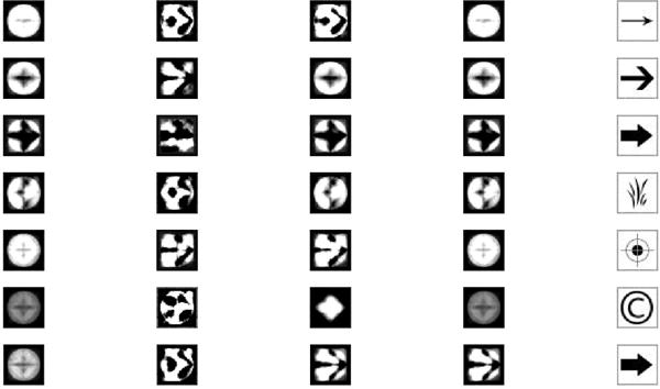
where ε ~ N(0, σ²). We fixed β₁ = β₂ = 0, α₁ = 0, and α₂ =−1. We consider an image pool consisting of 1457 two-dimensional images and randomly selected Z_i(·)′s from the pool. Figure 1 presents several randomly selected images.

Figure 1.

The image pool used in the second simulation setting.

We consider two scenarios for (θ, g). In both scenarios, we randomly selected an image from the image pool for each simulated data set. In the first scenario, we chose 7 images for θ from the image pool. For each θ image, we generated 1000 simulated data sets. In the second scenario, we generated 5,000 simulated data sets and randomly selected θ from the image pool in each simulated data set. We evaluated $\text{MNAR}({\widehat{k}}_n)$, MCAR, MAR and $\text{MNAR}(\widehat{\varphi },{\widehat{k}}_n)$ by using the prediction Bias and MISE₁, since they are close to Bias_n and MISE₂, respectively, in the second set.

Table 2 presents the simulation results for both scenarios. MNARs outperform MCAR and MAR, indicating that selecting the correct missing data mechanism can improve both prediction and estimation accuracy. Figure 2 presents some randomly selected estimated $\widehat{\mathit{\theta }}’\mathrm{s}$. These $\widehat{\mathit{\theta }}’\mathrm{s}$ can be quite different from θ since the basis functions constructed from FPCA may not accurately capture the variation of θ. However, for missing data problem, it remains largely unclear how to choose a set of efficient basis functions to accurately recover both the missing data and the functional signal. We will address this issue in our future research.

Table 2.

Simulation results based on 2-dimensional image covariates for the second simulation setting. Seven identification (ID) numbers were assigned to 7 randomly chosen images (see Figure 2) each producing 1000 replications of data sets. ID=’−’ indicates data set were generated with randomly chosen image coefficient in each replication.

test	ID	(ϕ, σ2),	(n, N/n)	MNAR( ${\widehat{k}}_n$)	MCAR	MAR	MNAR( $\widehat{\varphi },{\widehat{k}}_n$)
Bias	1	(1,.25)	(600,1/10)	0.060	0.077	0.071	0.059
MISE1	1	(1,.25)	(600,1/10)	0.636	0.901	0.704	0.634
Bias	2	(1,.25)	(1000,1/10)	0.063	0.081	0.076	0.062
MISE1	2	(1,.25)	(1000,1/10)	0.689	0.902	0.751	0.696
Bias	3	(1,.25)	(600,1/10)	0.064	0.082	0.076	0.063
MISE1	3	(1,.25)	(600,1/10)	0.731	0.958	0.770	0.737
Bias	4	(1,.25)	(600,1/10)	0.060	0.078	0.072	0.059
MISE1	4	(1,.25)	(600,1/10)	0.660	0.910	0.726	0.669
Bias	5	(1,.25)	(600,1/10)	0.060	0.078	0.072	0.059
MISE1	5	(1,.25)	(600,1/10)	0.642	0.899	0.701	0.649
Bias	6	(1,.25)	(600,1/10)	0.064	0.083	0.077	0.064
MISE1	6	(1,.25)	(600,1/10)	0.673	0.893	0.758	0.674
Bias	7	(1,.25)	(600,1/10)	0.064	0.082	0.076	0.064
MISE1	7	(1,.25)	(600,1/10)	0.733	0.934	0.767	0.741
Bias	–	(1,.25)	(600,1/5)	0.065	0.082	0.077	0.064
MISE1	–	(1,.25)	(600,1/5)	0.671	0.814	0.746	0.670
Bias	–	(1,.64)	(600,1/5)	0.114	0.200	0.192	0.113
MISE1	–	(1,.64)	(600,1/5)	0.707	1.141	0.960	0.708
Bias	–	(2,.25)	(600,1/5)	0.074	0.097	0.093	0.074
MISE1	–	(2,.25)	(600,1/5)	0.629	0.778	0.686	0.630
Bias	–	(1,.64)	(1000,1/3)	0.114	0.199	0.194	0.113
MISE1	–	(1,.64)	(1000,1/3)	0.676	0.885	0.867	0.676

Figure 2.

The selected 7 images in the second simulation setting—true value and their estimates. Images with IDs from 1 to 7 are shown in the 1st row to the 7th row, while the 5 columns represent the corresponding image estimates using the MNAR( ${\widehat{k}}_n$), MCAR, MAR, and MNAR( $\widehat{\varphi },{\widehat{k}}_n$)_, and the true image, respectively.

5. Application to the ADNI dataset

Alzheimer’s disease (AD) is the most common form of dementia and is an escalating national epidemic and a genetically complex, progressive, and fatal neurodegenetive disease. The ADNI study is a large scale multi-site study which has collected clinical, imaging, and laboratory data at multiple time points from cognitively normal controls (CN), individuals with significant memory concern (SMC), early mild cognitive impairment (EMCI), late mild cognitive impairment (LMCI), and subjects with AD. One of the goals of ADNI is to develop prediction methods to predict the longitudinal course of clinical outcomes (e.g., learning ability) based on imaging and biomarker data. More information about data acquisition can be found at the ADNI website (www.loni.usc.edu/ADNI).

To illustrate the empirical utility of our proposed methods in imaging classification, we use a subset of the ADNI data which consists of 682 subjects (208 CN controls, 153 AD patients, and 321 LMCI patients), after removing missing or low quality imaging data. Among them, there are 395 males with average age 75.38 years old and standard deviation 6.48 years old, and 287 females with average age 74.81 years old and standard deviation 6.81 years old. The T1-weighted images for all subjects at baseline were preprocessed by standard steps including AC (anterior commissure) and PC (posterior commissure) correction, N2 bias field correction, skull-stripping, intensity inhomogeneity correction, cerebellum removal, segmentation, and registration (Wang et al., 2011). Afterwards, we generated RAVENS-maps (Davatzikos et al., 2001) for the whole brain using the deformation field obtained during registration. We obtained the 256×256×256 RAVENS-maps and then down-sampled them to 128×128×128 for real data analysis.

The development of ETFLR is motivated by using imaging and clinical variables at baseline to predict clinical outcomes after baseline. The covariates of interest at baseline include age, gender, education, marriage status (married, divorced, or widowed), APOE4 (risk from variations of the APOE gene), DX-bl (CN, SMC, EMCI, LMCI, and AD), as well as the RAVENS map. The learning ability of each subject was scored (the so-called Rey Auditory Verbal Learning Test Score) at the 6, 12, 18, 24, and 30 months after baseline. The missingness rates of the test scores at the 18th, 24th and 30th month are very high, e.g., the missingness rate at the 18th month is 53.1%. We are interested in examining the learning ability at the 18th month, at which all LMCI and AD patients were tested for learning ability. We have 682 individuals in total, among which 362 individuals have missing data. It is necessary to model the missing responses given the high missingness rate.

We applied ETFLR to this ADNI data set as follows. First, to determine the tilting parameter ϕ, we obtained a validation set by investigating the responses at months other than the 18th month for those observations with missing responses. We interpolated the responses at the 18th month by using those at other months by a linear regression, and then we calculated the p−value associated with month. The interpolations with p-values less than .05 were considered as the validation set, and their corresponding interpolated responses were approximately taken as the missing true responses. By using both MNARN and MNARP (which are named in Subsection 2.2.3), we calculated two estimates of ϕ. Second, given $\widehat{\varphi }$, the first k_n components (columns) of the functional covariate Z, together with the non-functional covariates W (age, gender, etc.), we calculated the estimates of all coefficients by optimizing the quadratic form (2.8). We used GCV to choose k_n as in (2.10).

Third, we used RRSV to choose the optimal (h, w₀) as in (2.11). Given a grid of (h, w₀) values, we used the average prediction on the test set to choose the optimal (h, w₀). The criterion used is the Pearson correlation between the true and predicted responses. Specifically, we divided the dataset into half the test set and half the training set 500 times randomly, ensuring that both the missingness rate and the proportion of the validation set between the training set and the test set are the same. At each division, for every given h and w₀, we calculated, Cor_tr and Cor_test for all approaches, where Cor_tr is the correlation between the predicted responses and the true responses on the training dataset, and Cor_test is the correlation between the predicted responses and the true responses on the test dataset. After 500 divisions, we calculated their averages in comparison with MCAR and MAR approaches. See Table 3 for such results. We found that both MNARP and MNARN outperform in almost all tuning parameters (h, w₀)s’, and the best (h, w₀) is achieved at (1.1³h_min, 0.5) for MNARN. We also examine whether the functional covariate leads to better prediction. Specifically, by setting θ₀ = 0, we repeated the same estimation procedure to calculate (Cor_test, Cor_tr) at (1.1³h_min, 0.5), leading to Cor_tr = 0.257(0.054) and Cor_test = 0.127(0.059). Comparing such results with those in Table 3 reveals that RAVEN images can substantially improve prediction accuracy.

Table 3.

ADNI data analysis results: prediction accuracy scores.

	(w0, h)	MCAR	MAR	MNARP	MNARN
Cortr	(0, 1.13hmin)	.3238(.0695)	.2984 (.0658)	.2994 (.0654)	.2970 (.0619)
Cortest	(0, 1.13hmin)	.1161 (.0605)	.1384 (.0609)	.1388 (.0623)	.1377 (.0629)
Cortr	(0, 1.14hmin)	.3244(.0707)	.2993 (.0761)	.3000 (.0665)	.2967 (.0621)
Cortest	(0, 1.14hmin)	.1160 (.0607)	.1380 (.0608)	.1389 (.0615)	.1387 (.0624)
Cortr	(0, 1.15hmin)	.3243(.0701)	.2997 (.0672)	.3013 (.0674)	.2984 (.0633)
Cortest	(0, 1.15hmin)	.1150 (.0616)	.1373 (.0603)	.1384 (.0616)	.1377 (.0619)
Cortr	(0, 1.16hmin)	.3264(.0710)	.3010 (.0656)	.3031 (.0671)	.3014 (.0639)
Cortest	(0, 1.16hmin)	.1153 (.0613)	.1369 (.0592)	.1371 (.0604)	.1360 (.0611)
Cortr	(0, 1.17hmin)	.3269(.0706)	.3021 (.0665)	.3039 (.0678)	.3012 (.0635)
Cortest	(0, 1.17hmin)	.1146 (.0601)	.1368 (.0586)	.1373 (.0588)	.1368 (.0600)
Cortr	(1, 1.10hmin)	.3266(.0724)	.3023 (.0645)	.2949 (.0617)	.2900 (.0611)
Cortest	(1, 1.10hmin)	.1146 (.0620)	.1394 (.0586)	.1435 (.0593)	1419 (.0598)
Cortr	(1, 1.11hmin)	.3255 (.0695)	.3055 (.0672)	.2972 (.0627)	.2911 (.0633)
Cortest	(1, 1.11hmin)	.1152 (.0625)	.1404 (.0580)	.1459 (.0593)	.1447 (.0594)
Cortr	(1, 1.12hmin)	.3265(.0720)	.3069 (.0713)	.3009 (.0675)	.2944 (.0648)
Cortest	(1, 1.12hmin)	.1148 (.0609)	.1405 (.0577)	.1439 (.0587)	.1443 (.0589)
Cortr	(1, 1.13hmin)	.3266(.0731)	.3063 (.0720)	.3020 (.0695)	.2947 (.0647)
Cortest	(1, 1.13hmin)	.1139 (.0614)	.1393 (.0589)	.1438 (.0593)	.1447 (.0593)
Cortr	(1, 1.14hmin)	.3260(.0718)	.3064 (.0722)	.3032 (.0720)	.2972 (.0662)
Cortest	(1, 1.14hmin)	.1145 (.0613)	.1395 (.0588)	.1436 (.0598)	.1443 (.0594)
Cortr	(1, 1.15hmin)	.3268(.0726)	.3060 (.0685)	.3030 (.0691)	.2990 (.0668)
Cortest	(1, 1.15hmin)	.1147 (.0621)	.1398 (.0593)	.1433 (.0597)	.1445 (.0597)
Cortr	(1, 1.16hmin)	.3230(.0693)	.2997 (.0668)	.2998 (.0681)	.2957 (.0618)
Cortest	(1, 1.16hmin)	.1155 (.0609)	.1398 (.0609)	.1430 (.0612)	.1443 (.0616)
Cortr	(1, 1.17hmin)	.3277(.0720)	.3055 (.0689)	.3024 (.0688)	.2991 (.0677)
Cortest	(1, 1.17hmin)	.1139 (.0615)	.1363 (.0594)	.1404 (.0603)	.1405 (.0604)
Cortr	(1, 1.18hmin)	.3273(.0729)	.3052 (.0688)	.3026 (.0704)	.2996 (.0677)
Cortest	(1, 1.18hmin)	.1135 (.0614)	.1364 (.0595)	.1398(.0597)	.1388 (.0600)
Cortr	(0.5, 1.10hmin)	.3236(.0692)	.2999 (.0614)	.2908 (.0568)	.2888 (.0555)
Cortest	(0.5, 1.10hmin)	.1152 (.0615)	.1409 (.0598)	.1444 (.0597)	1433(.0607)
Cortr	(0.5, 1.11hmin)	.3243(.0705)	.3011 (.0653)	.2947 (.0619)	.2912 (.0594)
Cortest	(0.5, 1.11hmin)	.1150 (.0610)	.1413 (.0591)	.1443 (.0604)	.1436(.0621)
Cortr	(0.5, 1.12hmin)	.3242(.0685)	.3055 (.0695)	.3000 (.0670)	.2947 (.0614)
Cortest	(0.5, 1.12hmin)	.1157 (.0602)	.1415 (.0599)	.1462 (.0597)	.1462(.0616)
Cortr	(0.5, 1.13hmin)	.3232(.0702)	.3007 (.0694)	.2997 (.0683)	.2935 (.0613)
Cortest	(0.5, 1.13hmin)	.1163 (.0608)	.1418 (.0602)	.1461(.0599)	.1470 (.0613)
Cortr	(0.5, 1.14hmin)	.3234(.0700)	.3004 (.0704)	.3015 (.0692)	.2961 (.0630)
Cortest	(0.5, 1.14hmin)	.1163 (.0609)	.1412 (.0614)	.1453 (.0605)	.1464 (.0610)
Cortr	(0.5, 1.15hmin)	.3238(.0689)	.3027 (.0692)	.3014 (.0696)	.2965 (.0631)
Cortest	(0.5, 1.15hmin)	.1161 (.0601)	.1412 (.0607)	.1447 (.0606)	.1462 (.0613)
Cortr	(0.5, 1.16hmin)	.3237(.0702)	.2997 (.0666)	.3001 (.0679)	.2958 (.0616)
Cortest	(0.5, 1.16hmin)	.1158 (.0608)	.1409 (.0603)	.1438 (.0603)	.1447 (.0620)
Cortr	(0.5, 1.17hmin)	.3239(.0698)	.2993 (.0648)	.2984 (.0651)	.2945 (.0596)
Cortest	(0.5, 1.17hmin)	.1163 (.0607)	.1411 (.0604)	.1442 (.0601)	.1449 (.0599)
Cortr	(0.5, 1.18hmin)	.3248(.0702)	.2993 (.0653)	.2994 (.0655)	.2958 (.0591)
Cortest	(0.5, 1.18hmin)	.1149 (.0606)	.1390 (.0605)	.1422 (.0606)	.1423 (.0605)
Cortr	(0.5, 1.19hmin)	.3236(.0693)	.3001 (.0665)	.2997 (.0665)	.2979 (.0618)
Cortest	(0.5, 1.19hmin)	.1158 (.0608)	.1394 (.0605)	.1416 (.0612)	.1416 (.0616)

After fixing h = 1.1³h_min and w₀ = 0.5, we calculated the estimates of the non-functional covariates in Table 4. The bootstrap resampling procedure was further utilized for inference. Specifically, we repeated the bootstrap resampling procedure 300 times. At each time, we calculated the parameter estimates and $\widehat{\varphi }$. Subsequently, we calculated the 90% confidence intervals for ϕ and all other parameters and their associated p–values by using the Fast Double Bootstrap (Davidson and James, 2007). Table 4 also presents the bootstrap confidence intervals and their corresponding p–values based on MNARN. Table 5 presents the coefficient estimates for the four significant nonfunctional covariates and those for the principle components associated with the RAVEN images. Figure 3 presents the selected slices of the first two principle component images. We repeated the RRSV procedure and calculated the prediction accuracy (standard deviation) based on the test set for MCAR, MAR, MNARP, and MNARN as 0.143(0.063),0.154(0.062), 0.167(0.059), and 0.170(0.057), respectively. The results indicate that MNARN outperforms all other three methods.

Table 4.

ADNI data analysis results: parameter estimates, 90% confidence intervals and p-values of regression coefficients.

Covariates	MCAR	MAR	MNARP	MNARN	P-value
Age	−0.0157	−0.0059	0.0023	0.0112	0.56
	[−0.020, 0.059]	[−0.028, 0.021]	[−0.027, 0.035]	[−0.029,0.044]	–
Gender	0.0750	−0.1296	0.1014	0.2824	0.18
	[−0.804, 0.602]	[−0.546, 0.559]	[−0.516, 0.795]	[−0.546,0.969]	–
Education	0.0717	0.0714	0.0980	0.1276	0.00
	[−0.007, 0.145]	[.0004, 0.140]	[0.010, 0.201]	[0.005,0.209]	***
Apoe4	−0.3857	−0.3567	−0.4180	−0.4563	0.02
	[−0.551,−0.019]	[−0.594,−0.070]	[−0.728,−0.106]	[−0.817,−0.108]	**
if.widowed (marriage)	0.3891	0.3874	0.2955	0.2287	0.32
	[−0.303, 1.076]	[−0.191, 1.035]	[−0.265, 0.989]	[−0.316,0.980]	–
if.divorced (marriage)	1.2330	1.2590	1.4663	1.6364	0.04
	[0.405, 2.225]	[0.321, 2.201]	[0.418, 2.556]	[0.452,2.768]	**
if.lmci (DX-bl)	1.6478	1.7373	2.7110	3.4572	0.02
	[−0.135, 2.731]	[0.945, 3.069]	[1.309, 3.921]	[1.531,4.100]	**
$\widehat{\varphi }$	–	0	−0.1367	−0.2224
	–	0	[−0.292,−0.061]	[−0.392,−0.061]

Table 5.

ADNI: estimates for significant coefficients and their standard deviations in parentheses, and estimates for the top principle components.

	MCAR	MAR	MNARP	MNARN
Education	0.069 (0.046)	0.049 (0.044)	0.1101(0.053)	0.120 (0.055)
Apoe4	−0.379 (0.176)	−0.323 (0.169)	−0.3924(0.195)	−0.496 (0.216)
if.divorced (marriage)	1.158 (0.615)	1.118 (0.650)	1.3431(0.724)	1.500 (0.753)
if.lmci (DX-bl)	1.768 (0.958)	1.651 (0.556)	3.5929(0.613)	3.557(0.700)
1st.Pcomp	−0.227	−0.201	−0.314	−0.338
2ed.Pcomp	0	0.136	0.027	0
3ed.Pcomp	0	−0.090	−0.141	0
4th.Pcomp	0	0.178	0.0284	0
5th.Pcomp	0	0.202	0.060	0
6th.Pcomp	0	0.128	0	0
7th.Pcomp	0	0.041	0	0
8th.Pcomp	0	0.038	0	0
9th.Pcomp	0	−0.015	0	0
10th.Pcomp	0	−0.007	0	0

Figure 3.

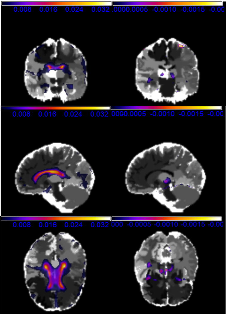
The first Principle Component (PC) of RAVEN images of ADNI real data analysis: positive loadings with the coronal slice at y = 62 (upper left), the sagittal slice at x = 71 (middle left), and the axial slice at z = 50 (lower left); negative loadings with the coronal slice at y = 66 (upper left), the sagittal slice at x = 71 (middle left), and the axial slice at z = 39 (lower left).

We have the following findings. First, MNAR performs well in both training and test sets for most window widths h and k_n. Second, the four covariates, Education, Apoe4, whether the individual is divorced, and whether the DX-bl of the individual is the LMCI (= 1) or the AD (= 0), strongly influence the learning test score. Such findings are clinically significant in that AD has a more serious effect on the intelligence behavior than LMCI. Third, the negative value of $\widehat{\varphi }$ in Table 4 implies that people with high learning test scores have the tendency to drop out of the study as expected. Finally, inspecting the functional coefficient image based on MNARN and MNARP (Table 5, Figures 3 and 5) reveals that estimates in most voxels are negative and relatively large in the regions of “lateral ventricle left” and “lateral ventricle right”. Such regions may have negative effects on learning ability. These findings are consistent with the existing literature on the abnormal lateral ventricle (Nestor, et.al. 2008) of AD patients.

Figure 5.

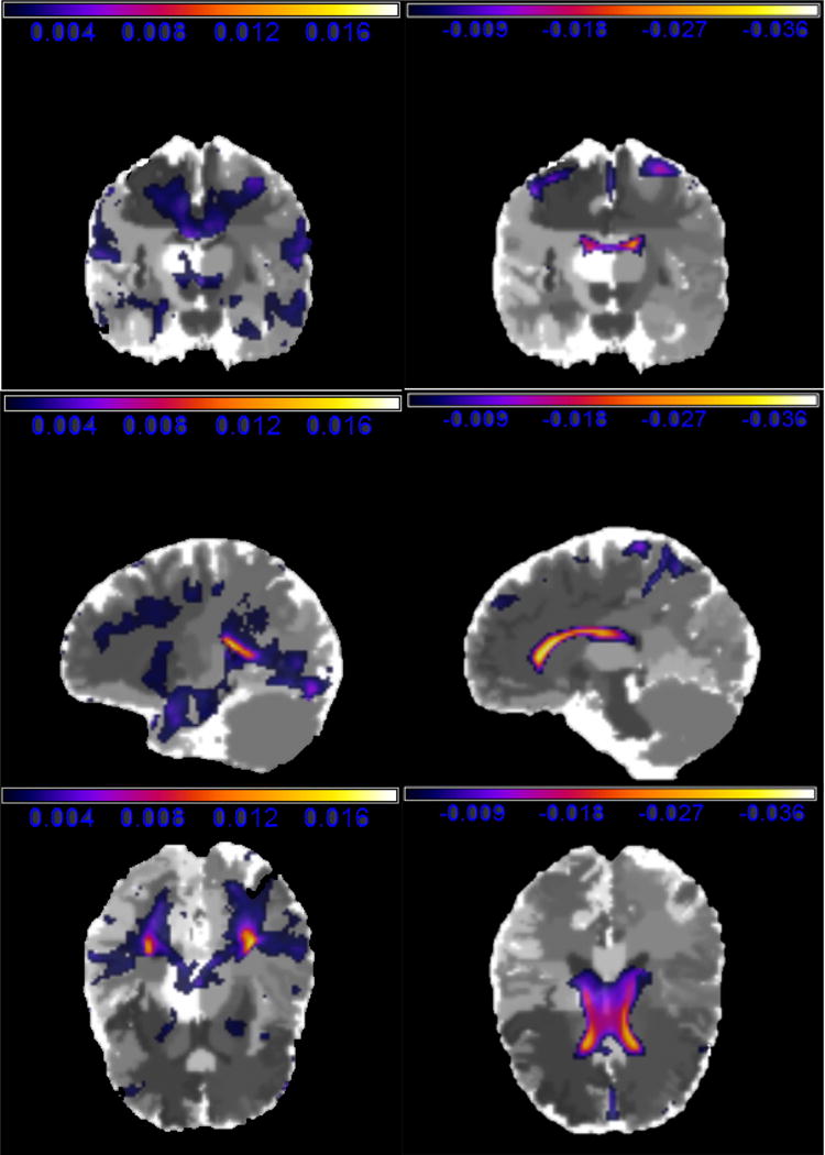
The functional coefficient images of MNARP of ADNI real data analysis: the positive part with the coronal slice at y = 62 (upper left), the sagittal slice at x = 76 (middle left), and the axial slice at z = 43 (lower left); the negative part with the coronal slice at y = 62 (upper left), the sagittal slice at x = 71 (middle left), and the axial slice at z = 50 (lower left).

Figure 4.

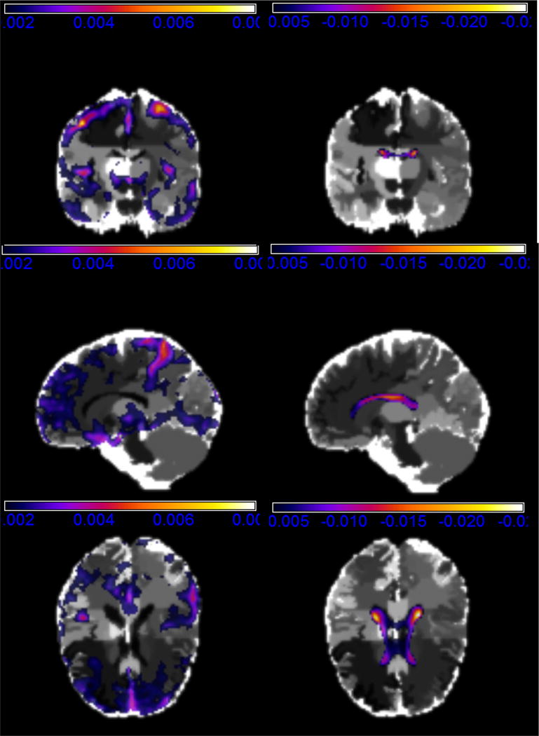
The second PC of RAVEN images of ADNI real data analysis: positive loadings with the coronal slice at y = 62 (upper left), the sagittal slice at x = 71 (middle left), and the axial slice at z = 50 (lower left); negative loadings with the coronal slice at y = 62 (upper left), the sagittal slice at x = 71 (middle left), and the axial slice at z = 50 (lower left).

References

- Baker SG, Laird NM. Regression analysis for categorical variables with outcome subject to nonignorable nonresponse. Journal of the American Statistical Association. 1988;83:62–69. [Google Scholar]
- Cai TT, Yuan M. Minimax and adaptive prediction for functional linear regression. Journal of the American Statistical Association. 2012;107:1201–1216. [Google Scholar]
- Cardot H, Ferraty F, Sarda P. Spline estimators for the functional linear model. Statistica Sinica. 2003;13:571–591. [Google Scholar]
- Cheng PE. Nonparametric estimation of mean functionals with data missing at random. Journal of the American Statistical Association. 1994;89:81–87. [Google Scholar]
- Chiou JM, Zhang YC, Chen WH, Chang CW. A functional data approach to missing value imputation and outlier detection for traffic flow data. Transportmetrica B: Transport Dynamics. 2014;2:106–129. [Google Scholar]
- Crambes C, André M. Asymptotics of prediction in functional linear regression with functional outputs. Bernoulli. 2013;19:2627–2651. [Google Scholar]
- Crambes C, Kneip A, Sarda P. Smoothing splines estimators for functional linear regression. The Annals of Statistics. 2009;37:35–72. [Google Scholar]
- Davatzikos C, Genc A, Xu D, Resnick SM. Voxel-based morphometry using the RAVENS maps: methods and validation using simulated longitudinal atrophy. NeuroImage. 2001;14:1361–1369. doi: 10.1006/nimg.2001.0937. [DOI] [PubMed] [Google Scholar]
- Davidson R, James GM. Improving the reliability of bootstrap tests with the fast double bootstrap. Computational Statistics & Data Analysis. 2007;51:3259–3281. [Google Scholar]
- Ferraty F, Sued M, Vieu P. Mean estimation with data missing at random for functional covariates. Statistics: A Journal of Theoretical and Applied Statistics. 2013;47:688–706. [Google Scholar]
- Ferraty F, Vieu P. Nonparametric Functional Data Analysis: Theory and Practice. Springer; New York: 2006. (Springer Series in Statistics). [Google Scholar]
- Ferraty F, Vieu P. Kernel regression estimation for functional data. In: Ferraty F, Romain Y, editors. The Oxford Handbook of Functional Data Analysis, Oxford Handbooks in Mathematics. Oxford University Press; Oxford: 2011. pp. 72–129. [Google Scholar]
- Friedman J, Hastie T, Tibshirani R. glmnet: Lasso and elastic-net regularized generalized linear models. 2009 R package version 1. [Google Scholar]
- Gillies RJ, Kinahan PE, Hricak H. Radiomics: images are more than pictures, they are data. Radiology. 2016;278:563–577. doi: 10.1148/radiol.2015151169. [DOI] [PMC free article] [PubMed] [Google Scholar]
- Hall P, Giles H. Truncated linear models for functional data. Journal of the Royal Statistical Society: Series B. 2015 To appear. [Google Scholar]
- Hall P, Horowitz JL. Methodology and convergence rates for functional linear regression. The Annals of Statistics. 2007;35:70–91. [Google Scholar]
- Hall P, Hosseini-Nasab M. On properties of functional principal components analysis. Journal of the Royal Statistical Society, Series B. 2006;68:109–126. [Google Scholar]
- Hall P, Hosseini-Nasab M. Theory for high-order bounds in functional principal components analysis. Mathematical Proceedings of the Cambridge Philosophical Society. 2009;146:225–256. [Google Scholar]
- Horvitz DG, Thompson DJ. A generalization of sampling without replacement from a finite universe. Journal of the American Statistical Association. 1952;47:663–685. [Google Scholar]
- Ibrahim JG, Chen MH, Lipsitz SR, Herring A. Missing-data methods for generalized linear models: a comparative review. Journal of the American Statistical Association. 2005;100:332–346. [Google Scholar]
- Ibrahim JG, Lipsitz SR, Chen M. Missing covariates in generalized linear models when the missing data mechanism is non-ignorable. Journal of the Royal Statistical Society: Series B. 1999;61:173–190. [Google Scholar]
- Ibrahim JG, Molenberghs G. Missing data methods in longitudinal studies: a review. Test. 2009;18:1–43. doi: 10.1007/s11749-009-0138-x. [DOI] [PMC free article] [PubMed] [Google Scholar]
- Kang JDY, Schafer JL. Demystifying double robustness: A comparison of alternative strategies for estimating a population mean from incomplete data. Statistical Science. 2007;22:523–539. doi: 10.1214/07-STS227. [DOI] [PMC free article] [PubMed] [Google Scholar]
- Kim JK, Yu CL. A semiparametric estimation of mean functionals with nonignorable missing data. Journal of the American Statistical Association. 2011;106:157–165. [Google Scholar]
- Kong D, Joseph GI, Lee E, Zhu H. Functional linear Cox regression models. 2015 doi: 10.1111/biom.12748. in submission. [DOI] [PMC free article] [PubMed] [Google Scholar]
- Li WV, Shao QM. Gaussian processes: Inequalities, small ball probabilities and applications. In: Shanbhag D, Rao C, editors. Stochastic Processes: Theory and Methods, volume 19 of Handbook of Statistics. Elsevier; New York: 2001. pp. 533–597. [Google Scholar]
- Little RJA. A note about models for selectivity bias. Econometrica. 1985;53:1469–1474. [Google Scholar]
- Little RJA, Rubin DB. Statistical Analysis With Missing Data. Wiley; New York: 2002. [Google Scholar]
- Martinez CA. Phd dissertation. Universidade de Santiago de Compostela; 2013. Estimates and bootstrap calibration for functional regression with scalar response. [Google Scholar]
- Molenberghs G, Kenward MG. Missing Data in Clinical Studies. Chichester: Wiley; 2007. [Google Scholar]
- Nestor SM, Rupsingh R, Borrie M, Smith M, Accomazzi V, Wells JL, Fogarty J, Bartha R, Alzheimer’s Disease Neuroimaging Initiative Ventricular enlargement as a possible measure of Alzheimer’s disease progression validated using the Alzheimer’s disease neuroimaging initiative database. Brain. 2008;131(9):2443–2454. doi: 10.1093/brain/awn146. [DOI] [PMC free article] [PubMed] [Google Scholar]
- Preda C, Saporta G, Hadj MMH. The NIPALS algorithm for functional data. Revue Roumaine de Mathematique Pures et Appliquees. 2010;55:315–326. [Google Scholar]
- Ramsay JO, Silverman BW. Functional Data Analysis. Second. John Wiley and Sons, Inc; 2006. [Google Scholar]
- Robins M, Rotnitzky A, Zhao L. Estimation of regression coefficients when some regressors are not always observed. Journal of American Statistical Association. 1994;89:846–866. [Google Scholar]
- Rotnitzky A, Lei Q, Sued M, Robins JM. Improved double robust estimation in missing data and causal inference models. Biometrika. 2012;99:439–456. doi: 10.1093/biomet/ass013. [DOI] [PMC free article] [PubMed] [Google Scholar]
- Shi X, Zhu H, Ibrahim JG. Local influence for generalized linear models with missing covariates. Biometrics. 2009;65:1164–1174. doi: 10.1111/j.1541-0420.2008.01179.x. [DOI] [PMC free article] [PubMed] [Google Scholar]
- Stewart GW. On the continuity of the generalized inverse. SIAM Journal on Applied Mathematics. 1969;17:33–45. [Google Scholar]
- Tang N, Zhao P, Zhu H. Empirical likelihood for estimating equations with nonignorably missing data. Statistica Sinica. 2014;24:723–747. doi: 10.5705/ss.2012.254. [DOI] [PMC free article] [PubMed] [Google Scholar]
- Van der Vaart AW. Asymptotic Statistics. Cambridge University Press; 2000. [Google Scholar]
- Van Der Vaart AW, Wellner JA. Weak Convergence and Empirical Processes. Springer; 2000. [Google Scholar]
- Wang D, Chen SX. Empirical likelihood for estimating equations with missing values. The Annals of Statistics. 2009;37:490–517. [Google Scholar]
- Wang Y, Nie J, Yap P, Shi F, Guo L, Shen D. Robust deformable-surface- based skull-stripping for large-scale studies. In: Fichtinger G, Martel A, Peters T, editors. Medical Image Computing and Computer-Assisted Intervention. Vol. 6893. Springer Berlin/Heidelberg; 2011. p. 635642. [DOI] [PubMed] [Google Scholar]
- Yao F, Müller HG, Wang JL. Functional linear regression analysis for longitudinal data. The Annals of Statistics. 2005;33:2873–2903. [Google Scholar]
- Zhao J, Shao J. Semiparametric pseudo likelihoods in generalized linear models with nonignorable missing data. Journal of the American Statistical Association. 2014;110:1577–1590. [Google Scholar]
- Zhou Y, Wan AT, Wang X. Estimating equations inference with missing data. Journal of the American Statistical Association. 2008;103:1187–1199. [Google Scholar]
Associated Data
This section collects any data citations, data availability statements, or supplementary materials included in this article.