Comparing dynamical systems concepts and techniques for biomechanical analysis

Abstract

Traditional biomechanical analyses of human movement are generally derived from linear mathematics. While these methods can be useful in many situations, they do not describe behaviors in human systems that are predominately nonlinear. For this reason, nonlinear analysis methods based on a dynamical systems approach have become more prevalent in recent literature. These analysis techniques have provided new insights into how systems (1) maintain pattern stability, (2) transition into new states, and (3) are governed by short- and long-term (fractal) correlational processes at different spatio-temporal scales. These different aspects of system dynamics are typically investigated using concepts related to variability, stability, complexity, and adaptability. The purpose of this paper is to compare and contrast these different concepts and demonstrate that, although related, these terms represent fundamentally different aspects of system dynamics. In particular, we argue that variability should not uniformly be equated with stability or complexity of movement. In addition, current dynamic stability measures based on nonlinear analysis methods (such as the finite maximal Lyapunov exponent) can reveal local instabilities in movement dynamics, but the degree to which these local instabilities relate to global postural and gait stability and the ability to resist external perturbations remains to be explored. Finally, systematic studies are needed to relate observed reductions in complexity with aging and disease to the adaptive capabilities of the movement system and how complexity changes as a function of different task constraints.

1. Introduction

Bernstein¹ presented research paradigms that led investigators to explore the rich patterns of movement that the human system is capable of producing. Traditional methods in biomechanics and motor control often have focused on discrete movement variables or linear relations in the times series of the components of the system. However, these methods lack the fidelity to fully explore this richness in movement patterns and led researchers toward a dynamical systems approach to the study of human behaviors. A dynamical system is one in which behaviors evolve over time. Current analysis methods from a dynamical systems perspective focus on the spatio-temporal evolution of the system dynamics over a period of time that can encompass steady state as well as abrupt qualitative changes in behavior.² Many of these analysis techniques derive from the study of nonlinear methods as opposed to the traditional linear approach. To illustrate the differences we will first discuss the distinction between linear and nonlinear methods.

Linear methods interpret the structure of data through linear correlations.³ The implication is that the intrinsic dynamics of a system are governed by the fact that small changes in the system result in small effects. Linear equations can only lead to solutions that decay, grow, or maintain a steady state. If we use as an example the population of an animal species (N), the linear equation will take the form of a straight line with growth rate R:

$$N_{i+1}=R{N}_i$$ (1)

where N_i is the present population value and N_i+1 is the value of N at the next instant in time (or generation). The system is decaying (i.e., N_i is getting smaller) when 0 < R < 1, growing (i.e., N_i is getting larger) when R > 1 and is at steady state (i.e., N_i remains constant) when R = 1. Traditional approaches in biomechanics are based in linear methods that have brought the discipline to its current state, but to move forward we need to incorporate alternative analysis techniques and interpretations.

Over the past several decades researchers have moved toward a dynamical systems approach to the study of human movement. In this case, human movement is determined by nonlinear responses. For example, tissues such as tendons show nonlinear characteristics in response to stretch. For our population example, these nonlinearities emerge when we make the growth rate R dependent on the population size through the function (R − bN_i); when the parameter b is positive the growth rate decreases as the population grows. This provides the following nonlinear finite difference equation:

$$N_{i+1}=(R-b{N}_i)N_i$$ (2)

Since the parameters R and b can vary independently, the only variable that can affect the dynamics of the system is:

$$x_i=\frac{b{N}_i}{R}$$ (3)

If we substitute x_i and x_i+1 into the previous equation, we get:

$$x_{i+1}=R{x}_i(1-x_i)$$ (4)

The nonlinear logistic equation is an example of a quadratic map and demonstrates how complex dynamics can result from (sometimes simple) nonlinear equations. In the logistic map we can observe steady state dynamics, bifurcations to periodic regimes, and chaotic dynamics that show bounded aperiodic behavior with sensitivity to initial conditions. These bifurcations and different system dynamics all occur as a function of a single parameter (R) change. Note that chaotic dynamics emerge in deterministic systems in which future states should formally be predictable but where uncertainty in initial conditions impacts prediction of future states. Human movement systems are not governed by these deterministic dynamics and more likely present stochastic behaviors governed by probabilities of states that can be impacted by deterministic and random processes.⁴

The formal examples above demonstrate the distinctive features of linear and nonlinear systems. By understanding these differences we can acknowledge that there are many physiological responses that have a nonlinear behavior: e.g., biological tissue, human behavior and human movement. These nonlinearities suggest that to accurately interpret human movement we should move toward nonlinear analyses. The dynamical systems approach focuses on how systems: (1) maintain their current state, addressing questions related to stability, (2) change or transition between states, addressing aspects of variability and adaptability, and (3) regulate complexity or fractal dynamics, characterized by interactions across different spatio-temporal scales as well as invariance of processes across these scales. Research on human movement in general and biomechanics in particular inspired by this dynamical systems approach has incorporated these concepts extensively but has often used terms such as stability, variability, and complexity interchangeably. The purpose of this paper is to compare and contrast the concepts of variability, stability, and complexity and how these impact movement adaptability. We will demonstrate that, although these concepts are clearly related, each presents different aspects of the system dynamics that requires careful a priori definition and consideration of their use in biomechanical research.

2. Variability and human movement

Many researchers have been concerned with the variability of movement.⁵ It has been demonstrated many times that, even with expert performers, movement behaviors cannot be replicated from one trial to the next with any degree of accuracy.⁶ Variability has been defined from a statistical point of view and is expressed as the variance (or the square root of the variance, that is, the standard deviation) about the mean.⁴ It should be noted that the variability of a performance may not simply be additive in the form of “measurement noise” but can be essentially part of the signal. The physiological variability or the actual variation from iteration to iteration can be explained by examining the following equations.³ If we define a system as:

$$x_{n+1}=F(x_n)$$ (5)

then the following equation adds measurement noise that is additive:

$$x_{n+1}=F(x_n)+{\mu }_n$$ (6)

where ${\mu }_n$ represents the process or measurement noise added to the system. Additive process noise can never be completely removed from the signal but can be attenuated using various signal processing techniques. However, the variability resulting from multiple trials of the same performance may actually be part of the signal and cannot be removed from the signal. This is expressed in the following equation:

$$x_{n+1}=F(x_n+{\beta }_n)$$ (7)

where ${\beta }_n$ characterizes “dynamical noise” instead of measurement noise and may represent inherent physiological variability that is part of the system dynamics.

While this definition is widely used for all sources of variation in a performance, the meaning of the variability must be understood in the context of the measurement. There are essentially two types of variability that can be determined: (1) end-point variability (i.e., the variability at the goal level) and (2) coordinative variability (i.e., how the performance was conducted over a number of iterations). End-point variability, the traditional focus of most research on variability, determines the outcome of the performance and has been used as an indicator of the level of performance skill. For example, in pistol shooting, keeping the barrel of the gun aimed precisely at a target with little or no variability is essential for the outcome (i.e., to hit the target accurately).⁷ However, low end-point variability (and high level of task performance) is not necessarily accompanied by low variability at the level of the coordinative dynamics. This was shown by Arutyunyan and colleagues⁷ in 1968 in an experiment on expert marksmanship performance (Fig. 1). Autocorrelation spectra show that the range of the gun amplitude is smaller for the expert while the range of the wrist and shoulder is greater in the expert in comparison to the more novice shooter.

Fig. 1.

End-point and joint space variability in novice (A) and expert marksman (B). The spectra of the autocorrelation functions as an individual prepares to shoot show less variation in end-point (gun) but more variation in joint space for the expert. The solid black lines represent the gun, the gray lines are the wrist joint, and the dotted lines are the shoulder.⁷

Adapted with permission.

The second type of variability, coordinative variability, plays an essential role in producing movement patterns that are adaptable and is observed during transitions between different modes, such as in bimanual manipulations and in gait.8, 9, 10, 11 From a Bernstein¹ perspective, coordinative variability is essential and critical in performance. Bernstein suggested that the same task may be accomplished using different degrees of freedom. Degrees of freedom, in this context, refer to the number of independent components (such as muscles, joints, segments) that are available to complete a task. The multiple degrees of freedom within a human system are what enable a performer to complete a task in various ways. Bernstein's insights into the utilized degrees of freedom may be captured by measuring segment and/or joint coordinative variability when completing a task. Thus, from a dynamical systems perspective, coordination variability is associated with the utilization of multiple ways of performing a task while higher levels of end-point variability are evidence of poor task performance.

Many researchers have examined coordination variability of segments and joints in different tasks from a dynamical systems perspective.12, 13, 14, 15 Based on these findings, coordination variability has been shown to be reduced under conditions of neurological disease and orthopedic injury, indicating a loss of flexibility in using coordination strategies to accomplish a task compared to healthy controls.¹⁶ Fig. 2 shows that two healthy groups of participants complete an unanticipated cutting maneuver.¹⁷ There was a significant difference in variability at 35%–45% and 0–100% of the performance with females having lower variability. The coordination variability in the female group is lower than in the male group, suggesting that the females may be at greater risk of injury as a result of the lower variability.

Fig. 2.

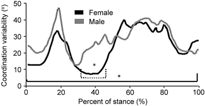
Coordination variability of a thigh rotation/leg rotation during an unanticipated cutting performance comparing males vs. females.¹⁷ * Indicates differences between females and males across the entire stance phase as well as in the 35%–45% range of stance.

Adapted with permission.

In many studies, variability is often used synonymously with stability and/or complexity. For example, increased variability in stride-to-stride intervals is often equated with loss of gait stability.¹⁸ As we shall see in the following sections, variability at the level of system output (e.g., stride-to-stride fluctuations during gait) or coordinative variability emerging from the interactions of joints or segments may relate to global measures of movement stability and complexity but should not be uniformly interpreted or equated with this stability or complexity.

3. Stability analysis of human movement

The term stability is frequently used within the context of research on human movement, yet its precise meaning varies. A general definition of stability is resistance to change. In dynamical systems, stability refers to a coordinative pattern's resilience to a change in response to a perturbation as measured by variance or deviation from the preferred or attractor state, or the ability to rapidly return to an attracter state (i.e., relaxation time).¹⁹ In postural control, stability entails maintenance of upright stance in response to unexpected external or self-generated perturbations, while gait demands that a dynamic component be considered. Certainly, an individual that falls due to a minor perturbation could be categorized as unstable. It is more difficult, however, to determine the degree of stability when a system displays sufficient resilience to the perturbation. That is, how close is the system to shifting into an unstable state? Various mathematical measures have been developed in an attempt to quantify a system's stability more precisely than the binary level of fall (unstable) vs. no fall (stable).

3.1. Global stability measures: center of mass (COM) and stability boundaries

In the study of human movement, stability is typically assessed by quantifying the vertical projection of the whole body COM as it relates to the base of support. This is termed global stability because it relates to a system's ability to maintain upright equilibrium by resisting large perturbations, such as slipping on a low friction surface or tripping over an obstacle.²⁰

Pai and Bhatt²¹ defined stability as the minimum distance between the COM motion state (position as a function of velocity) and a mathematically predicted feasible stability region boundary.²² Pai and Bhatt's stability measure accounts for both the instantaneous position and velocity of the COM. A similar measure of stability, originally developed by Hof and colleagues,²³ is the margin of stability. The margin of stability is calculated by subtracting the extrapolated COM (which takes into account both the horizontal position and velocity) from the anterior boundary of the base of support.24, 25 In a dynamical system, only regarding the COM position in relation to the base of support is insufficient in determining stability. That is, a system can be highly unstable while the COM is within the base of support if the COM velocity is rapidly approaching the stability boundaries. Alternatively, a system can be highly stable while the COM is outside of the base of support if the COM velocity is in the direction of the approaching stability boundaries and is of sufficient magnitude.²³ This is the case during locomotion, whereby whole body COM displacement necessitates transient changes in the base of support. The margin of stability is a valuable measure of stability because it is proportional to the impulse required to unbalance a system.²³ Thus, the margin of stability measure provides a quantitative degree of stability by explicitly stating the magnitude of perturbation required to destabilize the system. This suggests that an individual with a large margin value can withstand a greater perturbing impulse than an individual with a smaller margin, indicating greater stabilizing capacity.

Another technique for assessing static and dynamic stability is known as “time-to-contact”. This analysis is similar to the aforementioned stability measures evaluating the instantaneous COM position and velocity, yet also incorporates the COM acceleration to determine if the velocity is increasing, decreasing, or remaining constant.²⁶ By adding a 3rd dimension to the state space that contains potential stable states (i.e., all of the feasible combinations of COM positions, velocities, and accelerations that yield systemic stability), more information is available regarding instant current and future states. For example, an instantaneous COM motion state (position and velocity²¹) that is considered unstable may in fact be stable if the magnitude and direction of acceleration is sufficient. That is, if the COM is rapidly (high velocity) approaching the base of support, yet is also promptly slowing (negative acceleration), one may be able to predict that the COM will slow down or even reverse direction prior to crossing the base of support. This would indicate a stable system. Thus, the time-to-contact method may be considered a more complete description of the instantaneous state of the COM, and therefore potentially a more sensitive estimate of the time it will take to reach the base of support (Fig. 3).

Fig. 3.

Determination of dynamic stability using time-to-contact (TtC). This analysis evaluates the instantaneous position, velocity, and acceleration of the center of mass (COM) or center of pressure toward the physical base of support. Here shown for COM toward anterior and posterior boundaries of base of support in response to perturbation inducing forward body sway. Dashed arrow in lower panel indicates minimum TtC.⁶⁶

Adapted with permission.

In addition to direct measures of gait stability, gait cycle variance is a common indirect measure used to describe systemic gait stability. Gait research has shown evidence that falls are associated with higher relative variability in step length,²⁷ step width,²⁸ and stride time.18, 29 For this reason, these gait patterns are deemed unstable. What should be clearly stated, however, is that these associations do not provide evidence for causality. Thus, determining stability based on variability is, at best, an interpretation. In fact, studies have revealed opposing results regarding the relationship between variability and stability. Brach and colleagues³⁰ found that too little step width variability was as associated with falls as is too much step width variability. Dingwell and Marin²⁹ determined that slower walking speeds increased local dynamic stability (as assessed by Lyapunov analysis; see Fig. 4 and next section), even though stride-to-stride variability increased. Local dynamic stability can be defined as a locomotor system's resistance to infinitesimally small perturbations. Thus, while some of these variability measures have shown associations with falls (e.g., stride time fluctuations¹⁸), and may indeed possess a cause-and-effect relationship for future falls, more research is warranted to support this notion.

Fig. 4.

Evaluation of local dynamic stability using the finite-time Lyapunov exponent. A time series signal (A) is transformed into an Nth dimension state space (B; shown here as 3-dimensional) by adding a time delay (T) to the original signal. The state space reveals neighboring trajectories diverging as the behavior evolves. This divergence is a result of internal fluctuations or perturbations. On a logarithmic scale (C), the rate of short-term divergence over the course of a single stride (λ_ST) and long-term divergence from 4–10 strides (λ_LT) can be quantified by the slope of the solid lines of best fit. Higher rates of divergence are indicated by steeper slopes of the lines and indicate greater local instability.

3.2. Local stability measures based on nonlinear methods

In contrast to the global stability measures described in the previous section, researchers have also employed nonlinear methods in order to determine the “local” component of stability. Local dynamic stability can be defined as a system's sensitivity to small, intrinsic perturbations.³¹ That is, how well does the human locomotor system respond to naturally occurring fluctuations during gait? These fluctuations may be due to neuromotor noise or other internal perturbations, and must be attenuated in order to maintain global stability. One approach used in determining local dynamic stability is the maximal Lyapunov exponent (Fig. 4). This measure converts kinematic or kinetic data from a time series to a phase space (or state space) and determines the rates of convergence or divergence of nearby trajectories (here, the trajectory refers to the spatial path of the signal of interest within the state space; Fig. 4B). Determining true Lyapunov exponents requires a dataset of infinite time that is deterministic in nature (i.e., non-random). Therefore, appropriate assessment of experimental time series data entails evaluating the finite-time Lyapunov exponent.²⁰ This analysis determines the average rate (linear slope) of divergence on a logarithmic scale (Fig. 4C) over a finite-time window.³² The maximal finite-time Lyapunov exponent method may be considered more appropriate for gait data than other techniques because it does not assume precise periodic motion. An additional benefit of this analysis is that, unlike traditional measures of gait variability that treat each gait cycle as independent (i.e., variability across cycles is assessed in relation to the mean), the Lyapunov exponent evaluates the evolution of local locomotor stability over the course of several consecutive strides.²⁰ Importantly, the maximal Lyapunov exponent cannot be equated with overall variability in the system, as the latter reflects all of the variations (divergence and convergence) in the system and represents essentially different aspects of the system dynamics, while the maximal finite-time Lyapunov only assesses system divergence. Using this maximal finite-time Lyapunov analysis, Dingwell et al.²⁰ reported that patients with diabetic neuropathy were able to increase local dynamic stability by reducing their gait speed, even though this reduced speed was associated with greater stride-to-stride variability. Lockhart and Liu³³ noted that local dynamic stability was lower in older fall-prone adults when compared to young adults and older healthy adults during preferred speed walking.

Another method that evaluates a system's evolution and local orbital stability within its state space involves determination of maximal Floquet multipliers³⁴ (Fig. 5). This analysis first involves identifying a plane that is orthogonal to the mean of the state space cycle, whereby it transects all of the trajectories within the state space. This plane is known as a Poincaré section, and is used to determine whether the system's behavior is evolving to converge on or diverge from the mean of the state space (i.e., attractor state). The distance from the state space mean to the system at cycle (k) on the Poincaré section is compared to the distance from the mean to the subsequent cycle (k + 1). Floquet multipliers quantify this difference, and the maximal Floquet multipliers represent the degree of orbital stability. This analysis can be performed at one given point during a gait cycle, such as heel strike, or it can be evaluated over multiple portions of the gait cycle, such as 25%, 50%, or 75% of the gait cycle.³⁵ Using these Poincaré sections and Floquet multipliers, Granata and Lockhart³⁴ found that older fall-prone adults had more fluctuations from one foot strike to the next compared to young and older healthy adults.

Fig. 5.

The phase space analysis using a Poincaré section evaluates a signal's (S_k) evolution through a cycle to the subsequent cycle, S_k+1, in respect to the mean cycle (S*). If the signal is farther from the mean cycle than in the previous cycle (i.e., (S_k+1 – S*) > (S_k – S*)), the trajectory is diverging and the behavior is considered unstable.³⁵

Adapted with permission.

Another local nonlinear analysis method, Detrended Fluctuation Analysis (DFA), assesses the fractal structure and long-range correlation of fluctuations, and has also been shown to be associated with the stability or fall risk in individuals.¹⁸ The DFA is a modified root mean square analysis that divides an integrated time series into non-overlapping windows. Within each window the algorithm then fits a least square fit line, followed by detrending the data. The DFA for a given window size is the average root mean square deviation across the entire time series. The structure of the signal is then determined by the scaling exponent, α, which is the slope of the log-log plot of the DFA value for each window size (for a more detailed description of the algorithm see section on complexity below and Peng et al.³⁶). A scaling of α = 1 represents 1/f fractal-like long-range correlations that characterize optimal performance. Hausdorff et al.³⁷ used DFA on stride interval time during locomotion to determine that, compared to young adults, older adults and adults with Huntington's disease had reduced long-range correlations in stride fluctuations. That is, they exhibited more random behavior, while young adults exhibited long-range correlations of different time scales that approached the 1/f phenomenon. The 1/f phenomenon indicates long-term dependence across scales (i.e., a more fractal-like nature) and has been observed in physiological processes such as heart beat interval timing, and structures such as blood vessels and lungs.18, 38 This relationship is generally believed to represent a stable yet flexible system. However, as Dingwell and Cusumano³⁹ have shown, similar DFA values can be obtained by applying statistically independent auto-regressive models to the data. These authors showed similar DFA scaling exponents when applying surrogate data to the stride interval time series by using cross-correlated surrogates that preserve the auto-correlation and cross-correlation properties of the original data. That is, both surrogate data sets resulted in statistically similar DFA exponents for stride length and stride time. Indeed, the adequacy for the DFA analysis to determine long-range correlations requires further investigation. Moreover, the association between dynamic stability and fractal-like behavior (e.g., stride-to-stride variability) observed in human locomotion is still largely unknown.

3.3. Limitations of local stability measures

One of the major limitations of the paradigms used to assess local dynamic stability is that the evaluated systems are not externally perturbed and, as a result, their stability levels are not sufficiently probed. While these measures provide indirect evidence for a quantified degree of stability, the relationship between local stability and global stability or gait variability and global stability is currently unknown. More research is warranted that incorporates external perturbations to directly evaluate overall stability in order to justify (or invalidate) these nonlinear or variability-based stability measures.

Another issue of consideration is how the stability analysis features into the overall goal of the task as well as the timing of the activity. During a gait cycle, each instance does not need to be highly stable for the overall movement to be considered stable.³⁴ For example, a shift from quiet standing postures to walking (gait initiation) requires an unstable state whereby the COM is beyond the current base of support. If one were to examine a system during this behavioral shift (i.e., critical fluctuation¹⁹) out of context, the system would likely be deemed “unstable”. Yet evaluating the system from a more macroscopic perspective may reveal greater overall stability. It is important to note that the emergence of unstable states as during gait initiation may or may not lead to a fall event.²¹ Moreover, a locomotor system can be locally unstable yet globally stable during a gait cycle. That is, a system may not optimally resist infinitesimal fluctuations, yet still be of capacity to resist a large, finite disturbance. For example, the study by Dingwell and colleagues²⁰ revealed that patients with diabetic neuropathy had greater local dynamic stability, even though neuropathic patients have been known to have a much higher rate of falls, which would indicate lower global stability. Therefore, it is important to consider unstable dynamics during certain parts of the movement cycle or task in the context of the overall system performance and stability.

Finally, stability should be defined based on the constraints of the task. Although measures of stability are mathematically specific, the concept of stability from a functional perspective is often a subjective and relative term. For example, an individual that is perturbed during locomotion and is required to adopt a more lateral footstep to maintain balance could subjectively be considered stable because they did not fall, or unstable because they were forced to change footfall pattern. Additionally, they may be considered more or less stable than another person based on the amplitude of corrective stepping. However, this change in footfall pattern should only be considered unstable if the task constraints restrict this stepping strategy in maintaining balance. Otherwise, the change in step may be the most effective way to respond to the disturbance.²⁷ The relative aspect of stability is exemplified in the comparison of the maximal finite-time Lyapunov exponent and the state space analysis based on maximal Floquet multipliers. An individual may be considered locally unstable based on positive maximal finite-time Lyapunov exponents, yet considered locally stable based on maximal Floquet multipliers that are less than 1. This apparent paradox may be due to differences in time scales between analyses, such that Lyapunov exponents and Floquet multipliers evaluate fluctuations at shorter and longer time scales, respectively.⁴⁰ Still, this potentially confusing issue is a reminder that understanding the demands of the task will aid in determination of the most appropriate stability measures to use. To reiterate, dynamic stability should always be defined and considered within the context and demands of the task. We will now turn in more detail to nonlinear analysis methods that focus on assessment of dynamical processes at different spatio-temporal scales and interactions across these scales.

4. Methods to assess complexity in movement patterns

4.1. Fractal dynamics: correlations across multiple spatio-temporal scales

Physiological processes occur over a variety of spatio-temporal scales. The cooperative interaction among the processes, within and between scales, spontaneously gives rise to a mosaic of non-random, structured behavior; the newly emergent patterns of behavior constitute what is known as physiological complexity.41, 42, 43 A system is thought to be maximally complex when the log of its power spectrum has a 1/f^α=1 structure (long-range correlations); that is, the signal presents similar properties and correlational structure at different scales.⁴⁴ A perfectly correlated signal has an α = 1. When α = 0.5 movement fluctuations are considered random with no correlations (i.e., white noise). Long-range correlations that are persistent can be found in the range 0.5 < α ≤ 1.0 and anti-persistent correlations in the range α < 0.5. An α = 1.5 represents integrated white noise (brown noise) with only short range correlations, such as observed in Brownian motion.36, 44

Insights into the degree of complexity of the system can be gained through time series analysis of traditional gait and postural control variables such as inter-stride variability and center of pressure. As illustrated earlier, Hausdorff and colleagues⁴⁵ used DFA analysis to show that the variability observed in stride time intervals is not random (i.e., white noise) but follows an inverse power law distribution 1/f^α, where α ~ 1 (i.e., pink noise or long-range correlations). Similarly in free standing conditions, Duarte and colleagues44, 46 found that healthy individuals also exhibited this 1/f structure during quiet upright standing.

Pink noise is a pseudo random process whereby its evolution over time is influenced by the past and present behavior of the system. Here one cannot precisely predict its evolution, but distinct events based on probability distributions can be predicted. In a behavioral context this means that no repeated movement will be performed exactly the same, but essential properties of the movement will be similar across all repetitions.⁴⁷ Because the 1/f structure is temporally correlated across scales, any perturbation to one level will be reflected across the entire system, potentially leading to a reorganization of the body's degrees of freedom.⁴⁸ The ability to flexibly utilize different degrees of freedom to complete a task is a sign of systemic health, and a breakdown in the 1/f structure may point to the failing health of the system that is associated with a reduction in system complexity.47, 48, 49

Lipsitz and Goldberger⁵⁰ proposed the loss of complexity hypothesis as an explanation for loss of systemic stability with aging and disease. Within this hypothesis, aging and disease states act as constraints on the body's degrees of freedom, thereby reducing its complexity and ability to adapt to perturbations.⁵⁰ In this perspective reductions in effective degrees of freedom, interacting components and synergies become associated with a loss of variability and effective long-term correlations in the system. When these reductions in degrees of freedom, variability and correlational structure reach a critical threshold, injury or disease may emerge. Complexity, therefore, cannot be equated singly with variability of fluctuations about mean tendencies as has been implied in previous research.⁵¹ As pointed out by Lipsitz⁵² it is important to recognize the difference between variation in a signal and its complexity. For example, a reduction in the magnitude of variability, as reflected in the variation around the signal mean in Fig. 6, does not necessarily mean it is less complex.⁵²

Fig. 6.

Variability vs. complexity. Variation in a signal, such as the high amplitude deviation around the mean for the sine wave, cannot be equated with complexity. A signal can be variable but not complex (left panel), complex but not variable (middle panel), or variable and complex (right panel).⁵²

Adapted with permission.

4.2. Information theory and entropy

To measure the complexity of a biological system, movement scientists and physiologists have turned to tools from information theory. Information theory is a promising starting point because one of the main premises of the theory is focused on quantifying uncertainty. In the control of movement the coordination adopted by the body and the trajectory of the desired movement is sensitive to initial conditions. Because we seldom know the initial conditions of a body in space and how a movement will evolve, there is uncertainty in measurement. In information theory, the degree of uncertainty is measured by entropy, i.e., the amount of information needed to describe the system generating the information.⁵³

Kolmogorov–Sinai (K-S) complexity is a variant of Shannon's original information entropy, and serves as the basis for the most commonly used complexity algorithms. K-S entropy calculates the mean rate of new information when measured given the history of the system. This measure, however, requires large, noise free data sets.42, 54 Approximate entropy (ApEn) is among the most commonly used measures of complexity in the biomechanics literature,⁵⁵ and allows entropy calculations for finite data that contain noise (for more detailed information see Pincus and Goldberger⁵⁶). In the context of biomechanics, ApEn has been used to quantify postural control by assessing the complexity of center of pressure fluctuations under single and dual task paradigms,⁵⁷ and stride-to-stride variability in gait of patients with anterior cruciate ligament rupture.⁵⁸ This research has shown that the more regular the pattern the lower the ApEn value, and this lower entropy has typically been interpreted as less complex.57, 58

Despite the widespread use of ApEn in the biomechanics literature⁵⁵ the ApEn algorithm produces inconsistent results as it is sensitive to the length of the time series and provides a biased estimator of regularity because it self-matches (i.e., vectors are compared to themselves).⁴² Sample entropy (SampEn) is another family of entropy statistics that corrects for the pitfalls of ApEn; it also follows the same principles in that a large SampEn value is indicative of a more complex system. SampEn has been used to assess the regularity of posture control in patients with anterior cruciate ligament (ACL) injuries and of lower limb joint angles in high level athletes.59, 60

4.3. Multiscale sample entropy (MSE)

Despite their algorithmic differences, ApEn and SampEn are similar in that they assess entropy on a single spatio-temporal scale.⁴¹ As mentioned previously, the human body is organized in a hierarchical fashion with processes occurring on a variety of different time scales that interact with one another. To understand how constraints on the system (e.g., injury) impact its function it is important to consider the structure of the variability as well as the fluctuations occurring across all of the time scales. To address entropy changes across different time scales, Costa and colleagues41, 61 developed the MSE technique. The analysis first coarse grains the original time series through averaging points inside non-overlapping windows. The number of points being averaged inside of the window is dependent upon the number of scale factors being used; SampEn is then calculated on each newly created time-series. The result is a series of SampEn values across all time scales (Fig. 7).⁶¹ An advantage the MSE technique is that it allows a more detailed understanding of the physiological signal and may potentially identify differences in time scales that are contributing to the observed pattern of behavior. Research using the MSE technique has so far primarily focused on the overall impact of different time scales on the entropy measure. A priori insights into sensorimotor processes at different time scales and how different diseases and or expertise impact these are needed to optimally utilize the MSE approach.

Fig. 7.

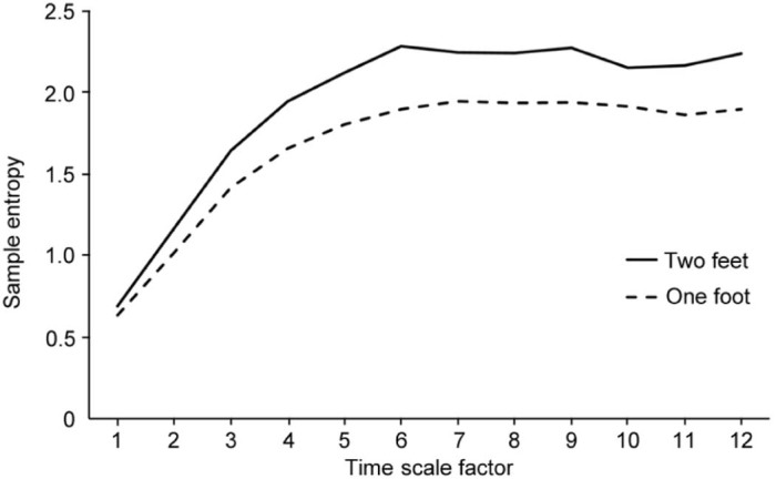
Example of multiscale sample entropy (MSE) output. The two curves represent the complexity of the center of pressure path length of an individual drumming a 1:1 anti-phase rhythm while standing on one and two feet. Time scale factors range from 12.5 ms (factor 1) to 150 ms (factor 12). It is important to note that the 1st scale factor is the sample entropy of the original time series, typically used in previous entropy analyses such as approximate entropy (ApEn). From the this graph it is clear to see that simply using a single time scale would underrepresent the processes operating at slower frequencies. The area under the curve is the overall complexity of the system (for more details, see reference⁶⁷).

Adapted with permission.

4.4. Entropy changes under different organism and task constraints

The loss of complexity hypothesis has been valuable in determining the impact of different organismic constraints that emerge as a function of aging and disease. A limitation of the current research using entropy is that it has been conducted primarily under steady state conditions, absent of behavioral context that we face on a daily basis.50, 62 To demonstrate that changes in complexity are task dependent, Vaillancourt et al.⁶² had young and older adults perform two force production tasks: (1) a constant force under isometric conditions, and (2) a sinusoidal force pattern over a given time course. Using ApEn, the results demonstrated that complexity patterns only partially abided by the loss of complexity hypothesis. That is, older adults demonstrated a loss of complexity in comparison to their younger counterparts when they were instructed to produce a constant force. However, this relationship changed when the task changed from static to variable (matching a sinusoidal force pattern).⁶² In the sinusoidal force matching task, older adults demonstrated increased complexity compared to younger participants. The increase in complexity as a function of constraints in older individuals may reflect a need for a larger number of degrees of freedom to be able to perform the task. Similar patterns of complexity change may be observed in expert performance.⁶²

In a recent study in our laboratory, expert marching percussionists performed two rhythms, the 1:1 anti-phase and a 2:3 poly rhythm at a self-selected slow and fast tempo (2:3-f), in two different postures (standing on one foot and two feet). MSE analysis of the path length of the center of pressure showed a reduction in complexity for the more constrained single foot compared to the two-footed posture (reduction in SampEn; Fig. 7). However, in the one-footed stance condition complexity increased when individuals were asked to perform a manual task (playing a 1:1 drumming rhythm) compared to quiet standing; further increases in complexity for the single leg posture only were also seen when the tempo of the task increased (playing a 2:3 vs. 2:3-f rhythm). This original reduction in complexity from a two-legged to a one-legged stance configuration, followed by an increase in complexity during the rhythmic drumming are in line with the proposed bi-directional hypothesis related to complexity changes put forth by Vaillancourt et al.⁶² in which complexity is task dependent. These findings suggest that a healthy system has the ability to freeze and release degrees of freedom as needed based on the imposed task constraints. Despite a difference in cohorts, the recent results from our laboratory (expert drummers) and those from Vaillancourt et al.⁶² (older vs. younger individuals) suggest that complexity may not always decrease as a function of organismic and task constraints, but can instead increase or decrease depending upon the constraints imposed.

5. Adaptability and human movement

The concepts of variability, stability, and complexity discussed so far are often associated with the notion of adaptability in human movement. A highly stable system, such as a limit cycle attractor or the in-phase coordination pattern observed in bimanual movements, is very difficult to perturb. Transitioning or adapting to a new constraint or behavioral state may be very challenging in these systems. Movement variability can play a role in destabilizing these patterns. Increased variability or fluctuations are essential features of abrupt changes (or phase transitions) in movement patterns. A signature feature of a phase transition is the appearance of fluctuations in the coordination pattern. These fluctuations are characterized by an increase in variability and deviation from intended coordination pattern (e.g., anti-phase oscillations), and a large increase in the time it takes to recover from a disturbance and return to steady state (i.e., critical slowing down).⁶³ Enhancement of fluctuations in complex systems arise due to influences of elements at a more microscopic level compared to the level of interest. These microscopic influences, together with environmental fluctuations, pull the system away from its current stable state or attractor. Fluctuations around the transition point have been observed during transitions in bimanual coordination from anti-phase to in-phase finger movements,⁶³ during gait in the transition between walking and running8, 64 and in coordination changes in the upper body and between arms and legs in human walking.⁶⁵

From these observations it is clear that there exists a link between the stability of a coordinative pattern and the ability of the system to transition to a new state and/or adapt to new constraints imposed. Therefore, a coordinative state that is too stable and resistant to perturbations may not be the most optimal state for flexible and adaptive movements to occur. The above described patterns in which 1/f type scaling occurs appear to contain the best mix of system dynamics in which fluctuations play a critical role in forming both short- and long-term correlations that allow for both stability and adaptability in the system.

The research described here clearly shows that variations in gait as measured by various stride parameters are not random but structured in some fashion, in which early fluctuations can have an impact on the gait dynamics at a later time. Changes in the structure of this variability (i.e., more random vs. more structured 1/f type self-similar noise) may possibly identify a loss of complexity and adaptability with disease.⁵⁰ Importantly, this claim requires further exploration in the human movement domain, as the link between gait patterns showing fractal fluctuations and gait adaptability has not been explored formally. The same is true for the assumed link between local dynamic stability as measured by Lyapunov exponents and overall gait stability and ability to adapt to perturbations; research on gait stability has not systematically identified these associations at this point.

6. Conclusion

In this paper we have reviewed fundamental concepts from a dynamical systems perspective as these relate to the variability, stability, and complexity of human movement. The purpose was to discuss the essential elements of and differences between the concepts of variability, stability, and complexity and how these impact movement adaptability. From this review, it is evident that these important concepts, although related, cannot be considered interchangeable and that future research should carefully distinguish between these. Variability both at the level of system output such as stride-to-stride fluctuations during gait or coordinative variability may relate to global measures of movement stability and complexity but should not be uniformly interpreted or equated with this stability or complexity. Current local dynamic stability measures using the finite-time maximal Lyapunov exponent can reveal local instabilities in movement dynamics, but the degree to which these local instabilities relate to global postural and gait stability and the ability to resist perturbations is still largely unknown. Therefore, observed reductions in local dynamic stability as measured by Lyapunov analysis will require empirical testing as to how these reductions impact ability to resist perturbations and change.

In addition, current methods such as DFA, Lyapunov analysis and various entropy techniques measure different aspects of the dynamics of the time series. We therefore strongly recommend that empirical research from a dynamical systems perspective should provide strong rationale and comparative argument for using certain analysis techniques over others. Finally, although research in human movement is beginning to show the reduction of complexity due to aging, injury, and disease, systematic studies are needed to assess and relate these reductions in complexity to adaptive capabilities of the movement system and how these complexity changes are related to different task constraints imposed.

Authors' contributions

All authors were involved in formulating the basic design and layout of the paper. RVE was responsible for the overall drafting of the paper; JH wrote introduction and variability sections; SWD wrote the stability and ACA the entropy section. All authors have read and approved the final version of the manuscript, and agree with the order of presentation of the authors.

Competing interests

None of the authors declare competing financial interests.

References

- 1.Bernstein N.A. Pergamon Press; Oxford: 1967. The co-ordination and regulation of movements. [Google Scholar]
- 2.Beek P., Peper C., Stegeman D. Dynamical models of movement coordination. Hum Mov Sci. 1995;14:573–608. [Google Scholar]
- 3.Kantz H., Schreiber T. 2nd ed. Cambridge University Press; Cambridge: 2004. Nonlinear time series analysis. [Google Scholar]
- 4.Riley M.A., Turvey M.T. Variability and determinism in motor behavior. J Mot Behav. 2002;34:99–125. doi: 10.1080/00222890209601934. [DOI] [PubMed] [Google Scholar]
- 5.Davids K., Glazier P., Araújo D., Bartlett R. Movement systems as dynamical systems. Sports Med. 2003;33:245–260. doi: 10.2165/00007256-200333040-00001. [DOI] [PubMed] [Google Scholar]
- 6.Preatoni E., Hamill J., Harrison A.J., Hayes K., Van Emmerik R.E.A., Wilson C. Movement variability and skills monitoring in sports. Sports Biomech. 2013;12:69–92. doi: 10.1080/14763141.2012.738700. [DOI] [PubMed] [Google Scholar]
- 7.Arutyunyan G.A., Gurfinkel V., Mirski M.L. Organization of movements on execution by man of an exact postural task. Biophysics (Oxf) 1968;14:1162–1167. [Google Scholar]
- 8.Diedrich F.J., Warren W.H., Jr Why change gaits? Dynamics of the walk-run transition. J Exp Psychol Hum Percept Perform. 1995;21:183–202. doi: 10.1037//0096-1523.21.1.183. [DOI] [PubMed] [Google Scholar]
- 9.Scholz J., Kelso J., Schöner G. Nonequilibrium phase transitions in coordinated biological motion: critical slowing down and switching time. Phys Lett A. 1987;123:390–394. [Google Scholar]
- 10.Seay J.F., Haddad J.M., van Emmerik R.E.A., Hamill J. Coordination variability around the walk to run transition during human locomotion. Motor Control. 2006;10:178–196. doi: 10.1123/mcj.10.2.178. [DOI] [PubMed] [Google Scholar]
- 11.Van Emmerik R.E., Wagenaar R.C., Winogrodzka A., Wolters E.C. Identification of axial rigidity during locomotion in Parkinson disease. Arch Phys Med Rehabil. 1999;80:186–191. doi: 10.1016/s0003-9993(99)90119-3. [DOI] [PubMed] [Google Scholar]
- 12.Dierks T.A., Davis I. Discrete and continuous joint coupling relationships in uninjured recreational runners. Clin Biomech (Bristol, Avon) 2007;22:581–591. doi: 10.1016/j.clinbiomech.2007.01.012. [DOI] [PubMed] [Google Scholar]
- 13.Hamill J., Van Emmerik R.E.A., Heiderscheit B.C., Li L. A dynamical systems approach to lower extremity running injuries. Clin Biomech (Bristol, Avon) 1999;14:297–308. doi: 10.1016/s0268-0033(98)90092-4. [DOI] [PubMed] [Google Scholar]
- 14.Heiderscheit B.C. Movement variability as a clinical measure for locomotion. J Appl Biomech. 2000;16:419–427. [Google Scholar]
- 15.Wheat J.S., Glazier P.S. Measuring coordination and variability in coordination. In: Davids K., Bennett S., Newell K., editors. Movement systems variability. Human Kinetics; Champaign, IL: 2005. pp. 167–181. [Google Scholar]
- 16.Wilson C., Simpson S.E., Van Emmerik R.E.A., Hamill J. Coordination variability and skill development in expert triple jumpers. Sports Biomech. 2008;7:2–9. doi: 10.1080/14763140701682983. [DOI] [PubMed] [Google Scholar]
- 17.Pollard C.D., Heiderscheit B.C., Hamill J., Van Emmerik R.E.A. Gender differences in lower extremity coupling variability during an unanticipated cutting maneuver. J Appl Biomech. 2005;21:143–152. doi: 10.1123/jab.21.2.143. [DOI] [PubMed] [Google Scholar]
- 18.Hausdorff J.M. Gait dynamics, fractals and falls: finding meaning in the stride-to-stride fluctuations of human walking. Hum Mov Sci. 2007;26:555–589. doi: 10.1016/j.humov.2007.05.003. [DOI] [PMC free article] [PubMed] [Google Scholar]
- 19.Kelso J., Ding M. Fluctuations, intermittency, and controllable chaos in biological coordination. In: Newell K.M., Corcos D.M., editors. Variability and motor control. Human Kinetics; Champaign, IL: 1993. pp. 291–316. [Google Scholar]
- 20.Dingwell J., Cusumano J., Sternad D., Cavanagh P. Slower speeds in patients with diabetic neuropathy lead to improved local dynamic stability of continuous overground walking. J Biomech. 2000;33:1269–1277. doi: 10.1016/s0021-9290(00)00092-0. [DOI] [PubMed] [Google Scholar]
- 21.Pai Y.C., Bhatt T.S. Repeated-slip training: an emerging paradigm for prevention of slip-related falls among older adults. Phys Ther. 2007;87:1478–1491. doi: 10.2522/ptj.20060326. [DOI] [PMC free article] [PubMed] [Google Scholar]
- 22.Pai Y.C., Wening J., Runtz E., Iqbal K., Pavol M. Role of feedforward control of movement stability in reducing slip-related balance loss and falls among older adults. J Neurophysiol. 2003;90:755–762. doi: 10.1152/jn.01118.2002. [DOI] [PubMed] [Google Scholar]
- 23.Hof A., Gazendam M., Sinke W. The condition for dynamic stability. J Biomech. 2005;38:1–8. doi: 10.1016/j.jbiomech.2004.03.025. [DOI] [PubMed] [Google Scholar]
- 24.Barrett R.S., Cronin N.J., Lichtwark G.A., Mills P.M., Carty C.P. Adaptive recovery responses to repeated forward loss of balance in older adults. J Biomech. 2012;45:183–187. doi: 10.1016/j.jbiomech.2011.10.005. [DOI] [PubMed] [Google Scholar]
- 25.Carty C.P., Mills P., Barrett R. Recovery from forward loss of balance in young and older adults using the stepping strategy. Gait Posture. 2011;33:261–267. doi: 10.1016/j.gaitpost.2010.11.017. [DOI] [PubMed] [Google Scholar]
- 26.Remelius J., Hamill J., van Emmerik R.E. Prospective dynamic balance control during the swing phase of walking: stability boundaries and time-to-contact analysis. Hum Mov Sci. 2014;36:227–245. doi: 10.1016/j.humov.2014.04.001. [DOI] [PubMed] [Google Scholar]
- 27.Maki B.E. Gait changes in older adults: predictors of falls or indicators of fear? J Am Geriatr Soc. 1997;45:313–320. doi: 10.1111/j.1532-5415.1997.tb00946.x. [DOI] [PubMed] [Google Scholar]
- 28.Dean J.C., Alexander N.B., Kuo A.D. The effect of lateral stabilization on walking in young and old adults. IEEE Trans Biomed Eng. 2007;54:1919–1926. doi: 10.1109/TBME.2007.901031. [DOI] [PubMed] [Google Scholar]
- 29.Dingwell J.B., Marin L.C. Kinematic variability and local dynamic stability of upper body motions when walking at different speeds. J Biomech. 2006;39:444–452. doi: 10.1016/j.jbiomech.2004.12.014. [DOI] [PubMed] [Google Scholar]
- 30.Brach J., Berlin J., Van Swearingen J., Newman A., Studenski S. Too much or too little step width variability is associated with a fall history only in older persons who walk at or near normal gait speed. J Am Geriatr Soc. 2005;53:S133–4. doi: 10.1186/1743-0003-2-21. [DOI] [PMC free article] [PubMed] [Google Scholar]
- 31.Dingwell J.B., Cusumano J.P. Nonlinear time series analysis of normal and pathological human walking. Chaos. 2000;10:848–863. doi: 10.1063/1.1324008. [DOI] [PubMed] [Google Scholar]
- 32.Rosenstein M.T., Collins J.J., De Luca C.J. A practical method for calculating largest Lyapunov exponents from small data sets. Physica D. 1993;65:117–134. [Google Scholar]
- 33.Lockhart T.E., Liu J. Differentiating fall-prone and healthy adults using local dynamic stability. Ergonomics. 2008;51:1860–1872. doi: 10.1080/00140130802567079. [DOI] [PMC free article] [PubMed] [Google Scholar]
- 34.Granata K.P., Lockhart T.E. Dynamic stability differences in fall-prone and healthy adults. J Electromyogr Kinesiol. 2008;18:172–178. doi: 10.1016/j.jelekin.2007.06.008. [DOI] [PMC free article] [PubMed] [Google Scholar]
- 35.Kang H.G., Dingwell J.B. Effects of walking speed, strength and range of motion on gait stability in healthy older adults. J Biomech. 2008;41:2899–2905. doi: 10.1016/j.jbiomech.2008.08.002. [DOI] [PMC free article] [PubMed] [Google Scholar]
- 36.Peng C.K., Havlin S., Stanley H.E., Goldberger A.L. Quantification of scaling exponents and crossover phenomena in nonstationary heartbeat time series. Chaos. 1995;5:82–87. doi: 10.1063/1.166141. [DOI] [PubMed] [Google Scholar]
- 37.Hausdorff J.M., Mitchell S.L., Firtion R., Peng C., Cudkowicz M.E., Wei J.Y. Altered fractal dynamics of gait: reduced stride-interval correlations with aging and Huntington's disease. J Appl Physiol. 1997;82:262–269. doi: 10.1152/jappl.1997.82.1.262. [DOI] [PubMed] [Google Scholar]
- 38.Liebovitch L.S., Shehadeh L.A. George Mason University; Fairfax, VA: 2003. Introduction to fractals. NSF nonlinear methods in psychology workshop. [Google Scholar]
- 39.Dingwell J.B., Cusumano J.P. Re-interpreting detrended fluctuation analyses of stride-to-stride variability in human walking. Gait Posture. 2010;32:348–353. doi: 10.1016/j.gaitpost.2010.06.004. [DOI] [PMC free article] [PubMed] [Google Scholar]
- 40.Cusumano J.P., Dingwell J.B. Movement variability near goal equivalent manifolds: fluctuations, control, and model-based analysis. Hum Mov Sci. 2013;32:899–923. doi: 10.1016/j.humov.2013.07.019. [DOI] [PMC free article] [PubMed] [Google Scholar]
- 41.Costa M., Goldberger A.L., Peng C.K. Multiscale entropy analysis of complex physiologic time series. Phys Rev Lett. 2002;89:068102. doi: 10.1103/PhysRevLett.89.068102. [DOI] [PubMed] [Google Scholar]
- 42.Costa M., Goldberger A.L., Peng C.K. Multiscale entropy analysis of biological signals. Phys Rev E Stat Nonlin Soft Matter Phys. 2005;71:e021906. doi: 10.1103/PhysRevE.71.021906. [DOI] [PubMed] [Google Scholar]
- 43.Manor B., Costa M.D., Hu K., Newton E., Starobinets O., Kang H.G. Physiological complexity and system adaptability: evidence from postural control dynamics of older adults. J Appl Physiol. 2010;109:1786–1791. doi: 10.1152/japplphysiol.00390.2010. [DOI] [PMC free article] [PubMed] [Google Scholar]
- 44.Duarte M., Sternad D. Complexity of human postural control in young and older adults during prolonged standing. Exp Brain Res. 2008;191:265–276. doi: 10.1007/s00221-008-1521-7. [DOI] [PubMed] [Google Scholar]
- 45.Hausdorff J.M., Peng C.K., Ladin Z., Wei J.Y., Goldberger A.L. Is walking a random walk? Evidence for long-range correlations in stride interval of human gait. J Appl Physiol. 1995;78:349–358. doi: 10.1152/jappl.1995.78.1.349. [DOI] [PubMed] [Google Scholar]
- 46.Duarte M., Zatsiorsky V.M. On the fractal properties of natural human standing. Neurosci Lett. 2000;283:173–176. doi: 10.1016/s0304-3940(00)00960-5. [DOI] [PubMed] [Google Scholar]
- 47.West B.J., Shlesinger M. The noise in natural phenomena. Am Sci. 1990;78:40–45. [Google Scholar]
- 48.Van Orden G.C., Holden J.G., Turvey M.T. Self-organization of cognitive performance. J Exp Psychol Gen. 2003;132:331–350. doi: 10.1037/0096-3445.132.3.331. [DOI] [PubMed] [Google Scholar]
- 49.Keshner M.S. 1/f noise. Proc IEEE. 1982;70:212–218. [Google Scholar]
- 50.Lipsitz L.A., Goldberger A.L. Loss of “complexity” and aging: potential applications of fractals and chaos theory to senescence. JAMA. 1992;267:1806–1809. [PubMed] [Google Scholar]
- 51.Moraiti C.O., Stergiou N., Ristanis S., Vasiliadis H.S., Patras K., Lee C. The effect of anterior cruciate ligament reconstruction on stride-to-stride variability. Arthroscopy. 2009;25:742–749. doi: 10.1016/j.arthro.2009.01.016. [DOI] [PubMed] [Google Scholar]
- 52.Lipsitz L.A. Dynamics of stability the physiologic basis of functional health and frailty. J Gerontol A Biol Sci Med Sci. 2002;57:B115–25. doi: 10.1093/gerona/57.3.b115. [DOI] [PubMed] [Google Scholar]
- 53.Cover T.M., Thomas J.A. John Wiley & Sons; New York, NY: 2012. Elements of information theory. [Google Scholar]
- 54.Williams G.P. Joseph Henry Press; Washington, DC: 1997. Chaos theory tamed. [Google Scholar]
- 55.Yentes J.M., Hunt N., Schmid K.K., Kaipust J.P., McGrath D., Stergiou N. The appropriate use of approximate entropy and sample entropy with short data sets. Ann Biomed Eng. 2013;41:349–365. doi: 10.1007/s10439-012-0668-3. [DOI] [PMC free article] [PubMed] [Google Scholar]
- 56.Pincus S.M., Goldberger A.L. Physiological time-series analysis: what does regularity quantify? Am J Physiol. 1994;266:H1643–56. doi: 10.1152/ajpheart.1994.266.4.H1643. [DOI] [PubMed] [Google Scholar]
- 57.Cavanaugh J.T., Mercer V.S., Stergiou N. Approximate entropy detects the effect of a secondary cognitive task on postural control in healthy young adults: a methodological report. J Neuroeng Rehabil. 2007;4:42. doi: 10.1186/1743-0003-4-42. [DOI] [PMC free article] [PubMed] [Google Scholar]
- 58.Georgoulis A.D., Moraiti C., Ristanis S., Stergiou N. A novel approach to measure variability in the anterior cruciate ligament deficient knee during walking: the use of the approximate entropy in orthopaedics. J Clin Monit Comput. 2006;20:11–18. doi: 10.1007/s10877-006-1032-7. [DOI] [PubMed] [Google Scholar]
- 59.Preatoni E., Ferrario M., Donà G., Hamill J., Rodano R. Motor variability in sports: a non-linear analysis of race walking. J Sports Sci. 2010;28:1327–1336. doi: 10.1080/02640414.2010.507250. [DOI] [PubMed] [Google Scholar]
- 60.Rhea C.K., Kiefer A.W. Patterned variability in gait behavior: how can it be measured and what does it mean. In: Li L., Holmes M., editors. Gait biometrics: basic patterns, role of neurological disorders and effects of physical activity. Nova Science Publishers; Hauppauge, NY: 2014. pp. 17–44. [Google Scholar]
- 61.Costa M., Peng C.K., Goldberger A.L., Hausdorff J.M. Multiscale entropy analysis of human gait dynamics. Physica A. 2003;330:53–60. doi: 10.1016/j.physa.2003.08.022. [DOI] [PMC free article] [PubMed] [Google Scholar]
- 62.Vaillancourt D.E., Sosnoff J.J., Newell K.M. Age-related changes in complexity depend on task dynamics. J Appl Physiol. 2004;97:454–455. doi: 10.1152/japplphysiol.00244.2004. [DOI] [PubMed] [Google Scholar]
- 63.Kelso J., Scholz J., Schöner G. Nonequilibrium phase transitions in coordinated biological motion: critical fluctuations. Phys Lett A. 1986;118:279–284. [Google Scholar]
- 64.Lamoth C., Daffertshofer A., Huys R., Beek P. Steady and transient coordination structures of walking and running. Hum Mov Sci. 2009;28:371–386. doi: 10.1016/j.humov.2008.10.001. [DOI] [PubMed] [Google Scholar]
- 65.Wagenaar R.C., Van Emmerik R.E.A. Resonant frequencies of arms and legs identify different walking patterns. J Biomech. 2000;33:853–861. doi: 10.1016/s0021-9290(00)00020-8. [DOI] [PubMed] [Google Scholar]
- 66.Hasson C.J., Van Emmerik R.E.A., Caldwell G.E. Predicting dynamic postural instability using center of mass time-to-contact information. J Biomech. 2008;41:2121–2129. doi: 10.1016/j.jbiomech.2008.04.031. [DOI] [PMC free article] [PubMed] [Google Scholar]
- 67.Gow B.J., Peng C.K., Wayne P.M., Ahn A.C. Multiscale entropy analysis of center-of-pressure dynamics in human postural control: methodological considerations. Entropy. 2015;17:7926–7947. [Google Scholar]