ORCHESTRAL FULLY CONVOLUTIONAL NETWORKS FOR SMALL LESION SEGMENTATION IN BRAIN MRI

Abstract

White matter (WM) lesion identification and segmentation has proved of clinical importance for diagnosis, treatment and neurological outcomes. Convolutional neural networks (CNN) have demonstrated their success for large lesion load segmentation, but are not sensitive to small deep WM and sub-cortical lesion segmentation. We propose to use multi-scale and supervised fully convolutional networks (FCN) to segment small WM lesions in 22 anemic patients. The multiple scales enable us to identify the small lesions while reducing many false alarms, and the multi-supervised scheme allows a better management of the unbalanced data. Compared to a single FCN (Dice score ~0.31), the performance on the testing dataset of our proposed networks achieved a Dice score of 0.78.

1. INTRODUCTION

White matter (WM) lesions are prevalent in neurological disorders such as multiple sclerosis (MS), small vessel disease (SVD), anemia, and in the normal aging population [1]. Since identifying and quantitatively measuring white matter lesions is clinically beneficial to prevent disease progression and for evaluation of treatment efficacy, it is imperative to accurately detect and quantify them. It has been shown that accurate early white matter lesion evaluation could reduce cognitive decline in patients with heart disease [2] and overt stroke in anemia patients [3].

Fluid-attenuated inversion recovery (FLAIR) MR images are widely used to observe white matter lesions, which appear as higher signal intensities in voxels, and are referred to as white matter hyperintensities (WMH). Manual segmentation is time-consuming and subject to intra- and inter-subject variablity, especially for small lesion loads (< 5ml) [4]. In recent years, many semi- and fully automated algorithms have been developed by either requiring a threshold to cluster WMHs (unsupervised methods), or using hand-crafted features (supervised methods) [1]. However, the accuracy of these methods relies on the training dataset, which may need to be impracticaly large, or may not be universally applicable due to the heterogeneous nature of WMH [5]. In addition, most of the existing learning-based methods perform well on large lesion segmentation, but are not sensitive to the detection of small lesions [6], which are particularly prevalent in some populations such as normal aging and anemic groups.

Convolutional neural networks (CNNs) are the most popular deep neural network (DNN) architectures [7]. They have been used to automatically extract brain, to separate tissue types [8, 9], and for tumor and WMH segmentation [10] in MRI. While most biomedical segmentation applications were reported in patients with relatively large lesion loads (MS, dementia, et. al.), few have been applied to small lesions in deep white matter (DWM) and sub-cortical WM. Therefore, DWM lesion segmentation using machine learning or deep learning methods is quite challenging.

We propose to use orchestral fully convolutional networks (OFCN), i.e., multi-scale and supervised networks, to segment DWM and sub-cortical WM lesions in 22 anemic patients. The architecture parallels three fully convolutional networks (FCN) and fuses predicted probability maps to yield a final segmented result.

2. METHODS

2.1. Data description

The MRI images were acquired according to Good Clinical Practice. Informed consent was signed from all participants under a protocol approved by the Institutional Review Board at Children’s Hospital of Los Angeles. After excluding cystic lesions and severe CSF flow artifacts found on FLAIR images, our dataset consisted of 22 anemic patients (age=22.4 ± 4.0, 14F, 8M). MRI examinations were performed on a Philips Achieva 3 Tesla magnet using an 8-element head coil. T1-weighted images were acquired for co-registration, and 3D T2-weighted FLAIR images were collected using the following parameters: TE/TR= 250/4800 ms, FOV 256 × 256 × 123, resolution 1 × 1 × 1.3 mm.

2.2. Preprocessing and ground truth segmentation

Firstly, we linearly and affinely registered all FLAIR images to the 1mm³ Montreal Neurological Institute (MNI) atlas using FLIRT and FNIRT [11]. Then we performed brain extraction and bias field correction using BrainSuite. Since inhomogeneous magnetic fields causes intensity variations in different patients, we histogram matched to a randomly selected patient using MATLAB® Image Processing Toolbox™ before data normalization. Lastly, all the intensity values were normalized by rescaling to the range of [0, 1].

To generate the ground truth (GT), we semi-manually segmented lesions using an in-house MATLAB-based toolbox previously published [12], by two on-site raters in consensus (one Ph.D student with a biomedical imaging background and one medical graduate student). The number and location of each WMH was confirmed by an experienced board-certificated neuroradiologist. When the boundary of the lesion did not agree with the raters’consensus, we used ITK-SNAP to delineate it voxel-by-voxel.

2.3. Orchestral fully convolutional networks

FCN has been widely used in computer vision and achieved breakthrough performance in image semantic segmentation. The key concept of FCN is the use of a deconvolutional layer, which is implemented by upsampling and transpose convolution, instead of a fully connected layer, so that the network architecture is transformed into fully convolutional form. Simultaneously, each deconvolutional output is augmented by concatenating the corresponding convolutional output through a skip architecture to generate the segmentation map. Due to its architecture without fully connected layers, FCN can speed up the segmentation and learn the object’s shape robustly without restricting the input image size [13].

Nonetheless, there are some limitations for FCN to identify the boundaries of small lesions. First of all, because of the downsampling and upsampling in FCN, the feature score maps in hidden layers are sparser than the original inputs [14], which causes a loss of image details. It is difficult for FCN to perform an accurate segmentation that requires more contour details. Furthermore, FCN generates the segmentation results through transpose convolution, which may cause the misclassification of voxels in the regions containing small objects [14], therefore FCN is not sensitive to classify data with an unbalanced class ratio, which is very common in small lesion segmentation. Hence, traditional FCN usually performs poorly in small lesion segmentation.

A popular alternative to achieve accurate segmentation is through patch-wise sampling the original image so that the networks train and predict each voxel based on the local patch formed by that voxel with its neighborhood [15]. However, due to the repetitive computation for each voxel and its neighborhood during patch sampling, the computational complexity of the model significantly increases. Also, the patch size could limit the segmentation performance. While smaller patch sizes may lose contextual information, larger patch sizes may decrease accuracy at the voxel level [16].

To conquer such limitations, we present an advanced deep neural network based on multiple scale parallel fully convolutional networks.

• Unbalanced dataset and multiple scale sampling The total number of voxels for a high-resolution 3D FLAIR image is more than 7 million, while the one for the small lesions per patient is around 300-700. Hence, in our problem, we face an extremely unbalanced dataset that has a ratio of lesion and non-lesion which is nearly 14,000:1. In addition, a large enough number of FLAIR images acquired with the same imaging protocol and in the same cohort is not always available. To overcome these problems, we sample original images into non-overlapping 3D patches, which require less computation than overlapping patches, and train patches so that the inner patch class ratio is more balanced and the training set is large enough for valid training. Also, we choose to use multiple patch sizes to train the model and fuse the results to correct the bias caused by a single patch size.

• Network architecture The architecture of the OFCN is shown in Fig. 1. The system consists of three parallel FCNs, which process 3D patches of size 32³, 16³, and 8³ respectively. For each FCN (Fig. 1. A), it contains 15 convolutional layers, 3 max-pooling layers, and 3 deconvolutional (upsampling and transpose convolution, i.e., up-conv) layers. The details of each layer, including filter sizes, feature channels, and activation functions are shown in Fig. 1 B. All the FCNs are supervised by the ground truth (GT in Fig. 1, dashed line as inputs) to generate three single FCN pre-segmented results (PS Map1, 2 and 3). Lastly, high complexity models may cause overfitting, while a simple majority vote considering all the pre-segmented maps as having equal weights may be less accurate. Instead, we applied the Adaboost algorithm [17] with classification and regression tree (CART) [17] as the weak learners supervised by the GT in the fusion center. This will recursively split the potential lesion voxels (the union of the three pre-segmented maps) into the lesion and false alarm ones, based on the features extracted from the three pre-segmented maps, to yield the final segmentation results.

• Training procedure To train the network model, we used a stochastic gradient descent algorithm [18] to optimize the Dice loss function, with a batch size of 32 and learning rate of 0.1. We used a rectified linear unit (ReLU) function as the nonlinear activation function for each neuron, to prevent the vanishing gradient issue [19]. The initialization for the weights in each convolutional kernel used a random Gaussian distributionwhich has a zero mean and standard deviation of $\sqrt{1/m}$, where m is the connection number of each layer, so that the model can converge faster. We divided our dataset (22 samples) into 5,544, 44,352, and 3.55 million 3D patches based on different patch sizes, respectively, for training and testing. We used leave-one-out strategy and trained our model for 1000 epochs, where the system converged, and then selected the best performance model according to validation sets. The network models were implemented in Python with the TensorFlow and Keras libraries. For the fusion center, the probabilities of the potential lesion voxels and their neighborhoods in three pre-segmented maps were used as features to train the boosting model.

Fig. 1.

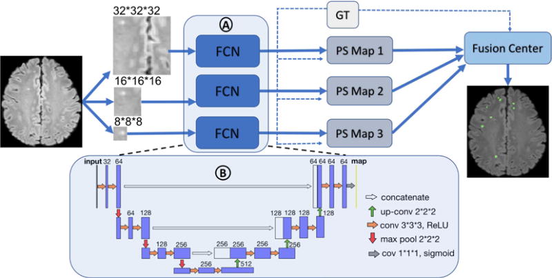
OFCN architecture: panel A encompasses three FCNs in parallel, and panel B represents the detail of the architecture of one single FCN in panel A. The FCNs are supervised by the ground truth (GT in Fig. 1, dashed line as inputs) to generate each of the pre-segmented maps (PS Map 1, 2, and 3). The fusion center combines all the pre-segmented maps based on the learning weights and threshold, also supervised by GT, to yield the final segmentation results.

2.4. Evaluations

To evaluate the performance of our OFCN system, we compared it to the single FCN (SFCN) model using three different patch sizes (SFCN-8, SFCN-16, and SFCN-32). In order to calculate the overlap between two segmentations, we used the Dice similarity coefficient (DSC) and average symmetric surface distance (ASSD, in mm) [20]. In addition, to compare lesion catch rate and false alarm rate, we also added recall and precision to the evaluation metrics to measure the proportion of true positives in the ground truth, and the proportion of true positives in the prediction, respectively.

3. RESULTS

Table 1 summarizes the performance of the individual FCN and OFCN. The sensitivity to lesion detection was excellent across all three patch sizes. In general, the DSC and precision increases while the ASSD dimension decreases with increasing patch size. Fig. 2 shows the comparison of the segmentation results from each of the models. Fig. 2 (c)-(e) indicate that reducing the patch size enhances the contour details of segmentation, but causes more false alarms. Our OFCN (Fig. 2 (f)) has less false alarms but better segmentation contours.

Table 1.

Evaluation results for 4 different architectures (All the metrics are reported as the average of all samples)

	DSC	ASSD (mm)	Recall	Precision
SFCN-32	0.70	11.0	0.90	0.61
SFCN-16	0.48	14.4	0.86	0.36
SFCN-8	0.16	17.1	0.90	0.09
OFCN	0.78	6.4	0.86	0.73

Fig. 2.

(a): T2-FLAIR image; (b): GT; (c)-(e): Segmentation of SFCN32, 16 and 8; (f): Segmentation of OFCN. The blue arrows point to the false alarms.

4. DISCUSSION

From the observation of sensitivity in Table 1, all the networks were sensitive to small lesions. Keeping high lesion catch rate as baseline, the similarity between segmentation and ground truth reflected the accuracy of segmentation. By comparing the SFCN results of different patch sizes in Table 1, larger patch sizes performed better than smaller patch sizes (DSC and precision decreased while ASSD increased), because more contextual information is included to correct for the false alarms caused by misclassification, due to the mixture of the tissue types or brain boundary. However, from Fig. 2 (c)-(e), it can be observed that smaller patch sizes had a higher accuracy to catch the lesion boundary. Over all, OFCN performed better than SFCN, because the orchestral model was more able to remove the false alarms based on the larger patch size models and corrected the contour bias of the smaller patch size models.

In a review of the literature [1], a DSC of 0.7 or higher is usually considered a good segmentation method. On the other hand, the comparisons of ASSD are not always valid, as different dataset and different GT segmentation were used for evaluation [20]. For comparison, we also tested the weighted cross entropy as loss function to account for the unbalanced data. However, there was no significant difference compared to our method. Our proposed OFCN for small lesion segmentation was able to achieve a DSC of 0.78. However, our method is not sensitive to the hyperintensities arised by CSF pulsatile flow artifact, or periventricular WMHs, due to the lack of location prior knowledge.

In conclusion, OFCN is capable of segmenting small WM lesions with a DSC of 0.78, while future test on different types of WM lesions in more diverse locations may help to further validate our proposed system. Scanning for this project is ongoing, and we will add more subjects as they become available to improve our validation.

References

- 1.Caligiuri ME, et al. Automatic detection of white matter hyperintensities in healthy aging and pathology using magnetic resonance imaging: A review. Neuroinformatics. 2015;13(3):261–276. doi: 10.1007/s12021-015-9260-y. [DOI] [PMC free article] [PubMed] [Google Scholar]
- 2.Bellinger DC, et al. Adolescents with tetralogy of fallot: neuropsychological assessment and structural brain imaging. Cardiology in the Young. 2015;25(2):338–347. doi: 10.1017/S1047951114000031. [DOI] [PMC free article] [PubMed] [Google Scholar]
- 3.DeBaun MR, et al. Controlled trial of transfusions for silent cerebral infarcts in sickle cell anemia. New England Journal of Medicine. 2014;371(8):699–710. doi: 10.1056/NEJMoa1401731. [DOI] [PMC free article] [PubMed] [Google Scholar]
- 4.Scheltens P, et al. White matter changes on ct and mri: an overview of visual rating scales. European neurology. 1998;39(2):80–89. doi: 10.1159/000007921. [DOI] [PubMed] [Google Scholar]
- 5.Eleftherios L, et al. T2 flair artifacts at 3-t brain magnetic resonance imaging. Clinical imaging. 2014;38(2):85–90. doi: 10.1016/j.clinimag.2013.10.004. [DOI] [PubMed] [Google Scholar]
- 6.Schmidt P, et al. An automated tool for detection of flair-hyperintense white-matter lesions in multiple sclerosis. Neuroimage. 2012;59(4):3774–3783. doi: 10.1016/j.neuroimage.2011.11.032. [DOI] [PubMed] [Google Scholar]
- 7.Schmidhuber J, et al. Deep learning in neural networks: An overview. Neural networks. 2015;61:85–117. doi: 10.1016/j.neunet.2014.09.003. [DOI] [PubMed] [Google Scholar]
- 8.Kleesiek JU, et al. Deep mri brain extraction: a 3d convolutional neural network for skull stripping. NeuroImage. 2016;129:460–469. doi: 10.1016/j.neuroimage.2016.01.024. [DOI] [PubMed] [Google Scholar]
- 9.Moeskops P. Automatic segmentation of mr brain images with a convolutional neural network. 2016;35(5):1252–1261. doi: 10.1109/TMI.2016.2548501. [DOI] [PubMed] [Google Scholar]
- 10.Kamnitsas K, et al. Efficient multi-scale 3d cnn with fully connected crf for accurate brain lesion segmentation. Medical image analysis. 2017;36:61–78. doi: 10.1016/j.media.2016.10.004. [DOI] [PubMed] [Google Scholar]
- 11.Smith SM, et al. Advances in functional and structural mr image analysis and implementation as fsl. Neuroimage. 2004;23:S208–S219. doi: 10.1016/j.neuroimage.2004.07.051. [DOI] [PubMed] [Google Scholar]
- 12.Vu CQ, et al. White matter hyperintensities segmentation and stereological bias correction. Proc ISMRM. 2016 [Google Scholar]
- 13.Long J, et al. Fully convolutional networks for semantic segmentation. Proc CVPR. 2015:3431–3440. doi: 10.1109/TPAMI.2016.2572683. [DOI] [PubMed] [Google Scholar]
- 14.Huang L, et al. Msfcn-multiple supervised fully convolutional networks for the osteosarcoma segmentation of ct images. Computer Methods and Programs in Biomedicine. 2017;143:67–74. doi: 10.1016/j.cmpb.2017.02.013. [DOI] [PubMed] [Google Scholar]
- 15.Ciresan D. Deep neural networks segment neuronal membranes in electron microscopy images. Advances in neural information processing systems. 2012:2843–2851. [Google Scholar]
- 16.Ronneberger O, et al. International Conference on MICCAI. Springer; 2015. U-net: Convolutional networks for biomedical image segmentation; pp. 234–241. [Google Scholar]
- 17.Murphy KP. Machine Learning: A Probabilistic Perspective. Massachusetts Institute of Technology; 2012. Adaptive basis function models; pp. 543–588. [Google Scholar]
- 18.Bottou L. Proc COMPSTAT’2010. Springer; 2010. Large-scale machine learning with stochastic gradient descent; pp. 177–186. [Google Scholar]
- 19.Maas Andrew L, Hannun Awni Y, Ng Andrew Y. Rectifier nonlinearities improve neural network acoustic models. Proc ICML. 2013;30 [Google Scholar]
- 20.Taha AA, et al. Metrics for evaluating 3d medical image segmentation: analysis, selection, and tool. BMC medical imaging. 2015;15(1):29. doi: 10.1186/s12880-015-0068-x. [DOI] [PMC free article] [PubMed] [Google Scholar]