Estimating organ doses from tube current modulated CT examinations using a generalized linear model

Abstract

Purpose

Currently, available Computed Tomography dose metrics are mostly based on fixed tube current Monte Carlo (MC) simulations and/or physical measurements such as the size specific dose estimate (SSDE). In addition to not being able to account for Tube Current Modulation (TCM), these dose metrics do not represent actual patient dose. The purpose of this study was to generate and evaluate a dose estimation model based on the Generalized Linear Model (GLM), which extends the ability to estimate organ dose from tube current modulated examinations by incorporating regional descriptors of patient size, scanner output, and other scan‐specific variables as needed.

Methods

The collection of a total of 332 patient CT scans at four different institutions was approved by each institution's IRB and used to generate and test organ dose estimation models. The patient population consisted of pediatric and adult patients and included thoracic and abdomen/pelvis scans. The scans were performed on three different CT scanner systems. Manual segmentation of organs, depending on the examined anatomy, was performed on each patient's image series. In addition to the collected images, detailed TCM data were collected for all patients scanned on Siemens CT scanners, while for all GE and Toshiba patients, data representing z‐axis‐only TCM, extracted from the DICOM header of the images, were used for TCM simulations. A validated MC dosimetry package was used to perform detailed simulation of CT examinations on all 332 patient models to estimate dose to each segmented organ (lungs, breasts, liver, spleen, and kidneys), denoted as reference organ dose values. Approximately 60% of the data were used to train a dose estimation model, while the remaining 40% was used to evaluate performance. Two different methodologies were explored using GLM to generate a dose estimation model: (a) using the conventional exponential relationship between normalized organ dose and size with regional water equivalent diameter (WED) and regional CTDI _vol as variables and (b) using the same exponential relationship with the addition of categorical variables such as scanner model and organ to provide a more complete estimate of factors that may affect organ dose. Finally, estimates from generated models were compared to those obtained from SSDE and ImPACT.

Results

The Generalized Linear Model yielded organ dose estimates that were significantly closer to the MC reference organ dose values than were organ doses estimated via SSDE or ImPACT. Moreover, the GLM estimates were better than those of SSDE or ImPACT irrespective of whether or not categorical variables were used in the model. While the improvement associated with a categorical variable was substantial in estimating breast dose, the improvement was minor for other organs.

Conclusions

The GLM approach extends the current CT dose estimation methods by allowing the use of additional variables to more accurately estimate organ dose from TCM scans. Thus, this approach may be able to overcome the limitations of current CT dose metrics to provide more accurate estimates of patient dose, in particular, dose to organs with considerable variability across the population.

1. Introduction

There has been excellent progress in estimating patient dose from body CT scans with the development of the size specific dose estimates (SSDE), published by AAPM Task Group 204.¹ However, these estimates were primarily determined from fixed tube current scans, while the vast majority of clinical body scans use some form of automatic exposure control (AEC) such as TCM. With TCM widely implemented and used as a dose reduction technique, it is important to be able to accurately quantitate and assess dose from these types of scans. In addition, SSDE refers to an average dose in the middle of the scan volume and dose to a homogenous, soft‐tissue‐like region (the abdomen). For that reason, SSDE is not necessarily a good predictor of dose that is organ‐specific per se, not even in the abdomen and especially not in other regions of the body.

While there have been attempts to estimate patient dose from TCM scans, each approach has had its limitations. One challenge is that while all manufacturers have implemented some form of TCM and all adjust tube current as a function of patient size and/or attenuation, the approaches vary substantially across manufacturers. McCollough et al.² described the different types of TCM algorithms that have been implemented to date, which include angular‐only modulation, longitudinal‐only (z‐axis‐only) modulation and a combination of angular and longitudinal. They also describe several user‐set “control parameters” such as Quality Reference mAs (Siemens, Philips), Noise Index (GE), and standard deviation (Toshiba). In addition, some manufacturers allow the user to set minimum and maximum tube current values, a circumstance which further complicates the characterization of TCM profiles. Developing a generalizable approach for estimating dose from TCM scans, in this very heterogeneous environment, is quite challenging.

There have been several analytical efforts to develop a general TCM function based on the basic principles of TCM as a function of patient attenuation. Schlattl et al.,^{3, 4} published dose conversion coefficients for seven voxelized phantom models spanning a range of body habitus and sex, from infants to adults, and using idealized TCM profiles based on Gies⁵ and Kalender et al.^{6, 7} While fundamental concepts of TCM may be applicable across CT systems, they differ from the theoretical definition, as described by Gies and Kalender, in manufacturer implementation, in operational parameters available for user selection, and in clinical practice.

Other studies have used Monte Carlo based software programs such as the ImPACT dosimetry calculator and PCXMC to estimate organ dose from TCM scans. Israel et al.⁸ used ImPACT and estimated dose to 91 patients who underwent tube current modulated CT exams by computing dose for each image, using extracted tube current values from the DICOM header of image data, and summing for whole‐organ and whole‐body dose estimates. The patient size limitation of ImPACT was overcome by establishing weight correction factors for different anatomical regions. In addition to the limitation of geometrical phantom used in this study, the difference between actual dose and the estimated dose is unknown and could not be assessed.

He et al.⁹ used PCXMC 2.0.1 to investigate how x‐ray tube current modulation affects patient dose in chest CT examinations using weighting factors for each projection. The investigated TCM function was theoretical and based on the basic principles of TCM technique, but was neither specific to any one manufacturer's algorithm nor to what is used in clinical practice. The theoretical TCM profiles were modeled as a function of x‐ray tube angle binned into 15° intervals, and longitudinal axis of the patient. In contrast, manufacturer algorithms use finer angular intervals (about 0.03°), and some manufacturers also incorporate empirical data derived from observer studies to generate patient‐specific TCM functions.

Angel et al.^{10, 11} used tube current values extracted from the raw projection data of actual clinical scans to account for TCM in the Monte Carlo simulations by changing the weight of each simulated photon based on the TCM data. The authors investigated the amount of dose savings in lungs and breasts from using TCM as compared to fixed tube current. This study was performed on a limited number of patients and the TCM data were all from one manufacturer's CT scanner model.

In another recent publication, Tian et al.¹² developed a model to estimate organ dose for clinical chest and abdominopelvic scans using a library of computational phantoms which were utilized to match a selected clinical patient. In this study, the authors used a previously developed¹³ theoretical TCM model with the XCAT patient models. Although they were able to generate TCM profiles, these profiles were theoretical and did not take scanner limitations and actual implementations into account, resulting in TCM profiles that were reasonably different from those reported elsewhere in the literature (Figures 3 and 8 of Angel et al.,¹⁰ Figure 1 of Angel et al.,¹¹ and Figures 2 and 12 in Khatonabadi et al.¹⁴). In addition, the developed dose estimation model was limited in that it was based on a scanner from a single CT manufacturer. A more recent publication by the same author uses the same library of computational phantom to estimate dose to 60 adult patients using the same previously developed theoretical TCM model¹³ with different modulation strength.¹⁵

Papadakis et al.¹⁶ recently published a method for estimating dose to primarily exposed organs in pediatric CT, taking into account TCM by implementing tube current values available in the DICOM header of individual images. Although the TCM functions utilized in the simulations were from actual clinical studies, they are representative of a single CT scanner system and TCM algorithm and not generalizable across different CT manufacturers. In addition, this paper only addresses dose from pediatric CT examinations.

To date, no studies have resulted in a generalizable method for estimating organ‐specific absorbed doses from tube current modulated CT exams beyond the specific patient or phantom populations used in the study. Hence, despite attempts to accurately estimate dose from tube current modulated scans, currently used dose metrics to assess dose from TCM exams are still scanner reported CTDI_vol, which represents an average CTDI_vol across the entire scan length, and more recently the size specific dose estimates from AAPM report 204¹ and 220.¹⁷

Thus, there is a need to develop a method to estimate organ dose from CT exams using TCM that utilizes accurate representations of actual TCM profiles and that is robust enough to cover a range of scanners from different manufacturers using different TCM algorithms. The approach described here extends previous approaches by developing a model that not only incorporates patient size and scanner output but also allows incorporation of other important factors. The factors investigated here include: (a) scanner manufacturer, which may help account for differences in TCM approaches and algorithms; (b) anatomic region, which may not only present different attenuation profiles in z plane (as well as x‐y plane), but may also invoke different TCM profiles that are adaptive to the anatomic region (e.g., chest TCM profiles may be different from abdominal/pelvic profiles) and (c) organ of interest, which may account for different regional attenuation and TCM profiles that are unique to the organ (e.g., the breast sub‐region as compared to the entire lung region). The general approach to model development will be to use estimates that are derived from Monte Carlo simulations using approaches previously described and validated.^{10, 11, 18, 19, 20, 21, 22, 23} The models being developed will use data from a wide variety of patient sizes, two different anatomic regions and TCM scan data from three different manufacturers.

Therefore, besides extending the results from previous publications,^{24, 25} which only used Siemens scanner data, to GE and Toshiba CT scanners, the purpose of this study was to utilize regional CTDI_vol and water equivalent diameter (WED)¹⁷ as a proxy for patient size, to develop a dose estimation model using the Generalized Linear Model. This is done using (a) the conventional exponential relationship between normalized organ dose and patient size metric as described in Eq. (1), and (b) using the same relationship along with additional predictors, called categorical variables, that will account for factors such as scanner manufacturer, anatomic region and even specific organ of interest. Both models were evaluated using a test set and compared against currently available dose estimates in the clinic.

$$NormalisedOrganDose=OrganDose/CTD{I}_{vol,Regional}=A{e}^{-B\times Patientsize},$$ (1)

where A and B are evaluated from GLM fit parameters.

2. Material and methods

The overall goal is to establish methods to estimate organ dose from CT exams utilizing TCM. With this work, methods will be developed and tested that account for patient size and scanner output using the conventional approach described by Turner et al.^{26, 27} and AAPM TG 204¹ as well as methods employing the generalized linear model (GLM) approach. GLM allows the incorporation of patient size and scanner output, in addition to other factors that account for patient‐specific, anatomic‐specific, and scanner‐specific factors and the complex interaction between an individual patient's anatomy and the TCM algorithms from different manufacturers. All models will be developed based on dose estimates provided by a validated Monte Carlo simulation approach that incorporates details of the scanner (e.g., spectral information, bowtie filter, geometry), patient information (organ locations based on actual scan image data), and TCM data (derived from patient scan data). The results of these simulations form the basis for both developing each dose estimation model and for testing the accuracy of the developed models.

2.A. Voxelized patient models

Voxelized patient models were generated from axial CT images acquired on three different CT scanner manufacturer models at four different institutions: (a) UCLA (Siemens data), (b) the MD Anderson Cancer Center in Houston, TX, (GE data) (c) UT Southwestern Medical Center (adult Toshiba data), and (d) Arkansas Children's Hospital (pediatric Toshiba data). All Siemens data were collected from three different Siemens Sensation 64 slice scanners with CareDose 4D software with “average” strength settings. GE data were collected from a single CT model, LightSpeed VCT, with Smart mA tube current modulation option. Toshiba data were collected from a single model CT, the Aquilion 64, with SUREExposure. Imaging parameters were variable among sites with most pediatric scanning performed with 100 kVp and adult imaging with 120 kVp. The institutional review board at each institution approved the collection of the data. The raw projections were only available from scans acquired at UCLA, and therefore, only those scans were used to extract detailed tube current information for use in the MC simulations. For all GE and Toshiba data, tube current value available in the DICOM header of each image was used to generate z‐axis only modulation (longitudinal modulation) profiles for each patient to use in TCM simulations. This approach has been previously shown to provide acceptable organ dose estimates when compared to estimates based on the detailed (angular and longitudinal) tube current data.¹⁴ Along with patient images, patient dose reports were also collected. Table 1 summarizes the types and numbers of clinical studies collected from the different CT scanners. A total of 332 patient data sets were collected for use in this study.

Table 1.

An overview of collected chest and abdomen/pelvis patient studies from different scanners

Patient cohort	Siemens (sensation 64)		GE (lightspeed VCT)		Toshiba (aquilion 64)
	Abd/Pel	Thorax	Abd/Pel	Thorax	Abd/Pel	Thorax
Male	30	29	10	10	15	17
Female	32	42	9	9	11	24
Pediatrics	20 (12 m, 8 f)	29 (16 m, 13 f)	5 (2 m, 3 f)	9 (3 m, 6 f)	13 (6 m, 7 f)	18 (11 m, 7 f)
Total	182		52		98

Patient images from scans on Siemens and GE scanners were reconstructed with 500 mm field of view to ensure body coverage throughout the entire scan length. All adult patients scanned on the Toshiba scanner from UT Southwestern Medical Center were either reconstructed at 500 or 400 mm FOV with only minimal or no cutoff of anatomy. All pediatric‐patient data from the Toshiba Aquilion 64 scanner at Arkansas Children's Hospital were collected retrospectively with no possibility of reconstructing the images at a larger FOV. These pediatric‐patient images were reconstructed using 200 mm to 400 mm FOV, which resulted in some cases having some missing anatomy (mostly fat and soft tissue). None of these patients had cutoffs within the regions/organs of interest (i.e., organs for which dose simulations were performed).

Liver, spleen, and kidneys were identified using semi‐automated contouring techniques in all abdomen/pelvis studies. Lungs and glandular breast tissues were contoured in all thorax studies, with the breast being segmented only in female patients. Segmented images were used to generate voxelized patient models as described in previous publications.^{10, 11} A total of 332 voxelized patient models were created for this study. From those voxelized patient models, a total of 714 organs were contoured. Figure 1 shows the range of patient sizes used in this study. Both patients were scanned on the same CT scanner and images were reconstructed using a 500 mm field of view.

Figure 1.

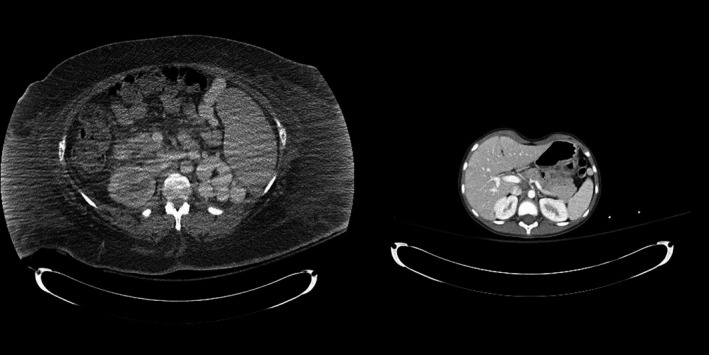
A visual illustration of the range of patient sizes used in this study.

2.B. Patient size metrics

Collected axial CT images were used to determine WED on an image by image basis. As shown in the previous publication,²⁵ with regard to the abdomen, no significant difference was observed in the numerical value of effective diameter and WED (Effective diameter is the diameter of a circle that has the same cross‐sectional area as the patient at a given z‐axis or longitudinal location. However, WED is the diameter of a cylinder of water with the same x‐ray absorption of a patient). However, for the thorax, a statistically significant difference between these metrics was observed, especially for estimation of dose to lungs, where the overall attenuation is significantly less than in a region of predominantly soft‐tissue organs of density comparable to that of water. In particular, regional WED showed a statistically significant improvement over effective diameter for estimating dose to lungs. Hence, regional WED was employed for creating dose estimation models in this study.

2.C. Monte Carlo simulation tool

The Monte Carlo software package MCNPX (Monte Carlo N‐particle eXtended version 2.7.0) was utilized for all the simulations.^{26, 28} The generic source code of MCNPX was modified to model a MDCT scanner geometry and spectrum.^{18, 19, 20, 21} The code is capable of selecting the appropriate energy spectrum data, previously generated using the “equivalent source” method by Turner et al.,²¹ and other user‐specified variables such as scan start, and scan length in a so‐called input file, an MCNPX‐generated text file with specific instructions on the path of individual photons.

In the case of TCM simulations, an additional text file with information on individual tube position, tube angle, and tube current value throughout the scan, which is either extracted from the raw projection data of actual CT scans or from the DICOM header of the images, is utilized in the simulation. Extensive validation of this MC simulation package under a wide variety of conditions including TCM has been previously reported.^{22, 23}

2.D. Generation of reference organ dose values

We used the Monte Carlo simulation tool (2.E..C) to generate organ dose values that will serve as reference values for the remainder of this work. For each patient model, the appropriate TCM functions were used and estimates were obtained for each of the segmented organs described above. In addition to the reference organ dose values, regional CTDI_vol, and regional WED were calculated for each patient. Regional CTDI_vol values were used to normalize the simulated reference organ dose values as described in Khatonabadi et al.²⁴

2.E. Development of dose estimation models

2.E.1. Generalizability of regional CTDI_vol across CT manufacturers

To verify the generalizability of the regional CTDI_vol across the CT scanner models studied, the conventional relationship between normalized organ dose and patient size was explored using two different normalization factors and WED as patient size metric: (a) CTDI_vol,_Regional (CTDI_vol value corrected to represent tube output at a specific region) and (b) CTDI_vol,Global (CTDI_vol value reported by the scanner based on an average tube current across the entire scan length). To examine each normalization factor, the log‐transformation of normalized organ dose is used to fit a linear regression with the covariate of WED. Different regression analyses were performed on differently categorized datasets; investigating scanner‐specific, organ‐specific, and pooled dataset fits. The coefficient of determination from the linear regression was reported to compare the appropriateness of each normalization factor (CTDI_vol,_Regional versus CTDI_vol,Global).

2.E.2. Overview of various dose estimation models

Once the generalizability of regional CTDI_vol across studied CT scanner models was established, dose estimation models using regional CTDI_vol and regional WED were developed. The conventional estimation model as used in generating conversion factors to calculate SSDE is a simple exponential model that describes the relationship between normalized phantom dose and effective diameter. While this approach has been shown to be very useful in estimating SSDE across a range of CT scan protocols,^{29, 30, 31} there remain some limitations in its ability to accurately estimate specific organ doses, such as dose to the glandular breast tissue, especially under TCM scanning conditions.

Therefore, to extend the model, a statistical method was investigated using the generalized linear model (GLM), a generalization of linear regression. Logarithmic transformation of dose values was used to meet the GLM assumption of a normally distributed response function.

With regard to this work, the response variable is the organ dose normalized by regional CTDI_vol and the predictors are WED, as in the conventional model described above in Eq. (1), as well as possible extensions to several sub‐categorical variables, such as scanner manufacturer models which includes individual categorical variables of Siemens Sensation 64, Toshiba Aquilion 64, and GE LightSpeed VCT, exam type (Chest or Abd/Pel), organs (lung, breast, liver, kidney, spleen), and patient sub‐categories (adults versus pediatrics). In our analysis, each of the categorical variables is binary, that is, each can take on the value 0 or 1. For instance, exam type abdomen/pelvis can either take on the value 1 for including the exam type to be abdomen/pelvis or it can be 0. A value of 1 indicates that the (logarithmically transformed) normalized organ dose data associated with that categorical variable are included in the linear regression, whereas a value of 0 indicates that the associated data are excluded from the linear regression.

The conventional dose estimation model is:

$$Ln(NormalizedOrganDose)=\mathit{\alpha }+({\mathit{\beta }}_1\times WED),$$ (2)

where $\mathrm{\alpha }$ is a constant and $rbet{a}_1$ is a coefficient of WED. By adding categorical variables, Eq. (2) can be rewritten as:

$$Ln(NormalizedOrganDose)=\mathit{\alpha }+\{({\mathit{\beta }}_1\times WED)+({\mathit{\beta }}_2\times \mathbf{scanner}(e.g.Siemens))+({\mathit{\beta }}_3\times \mathbf{Organ}(e.g.Breasts))+\dots \}$$ (3)

Table 2 highlights the two dose estimation models, their definitions, and their response variables. Differently constructed models were compared using adjusted R², correlations and significance of correlations. The regression analysis includes two‐sided P‐values used in testing coefficient predictors of the independent variables. STATA version 14.0 (College Station, TX 77845 USA) was used for the analyses.

Table 2.

Overview of the generated models along with their definitions and response variables

Model	Response variable	Independent variables	Categorical variables
GLM w/o categorical variables	Logarithm of organ dose normalized by Regional CTDIvol	Regional WED	None
GLM w/categorical variables		Regional WED + Categorical Variables	Scanners: Siemens Sensation 64, GE LightSpeed VCT, Toshiba Aquilion 64; Organs: liver, spleen, kidneys, breasts, lungs; Scanning Regions: abdomen/pelvis, chest; Adult sex: male, female; Pediatric Patient

2.F. Model training and testing

Monte Carlo simulations were performed for all 332 patients to obtain dose to 714 organs which were used as reference organ dose values. Patients were stratified by organ, gender, and scanner using their calculated WED into a training set of 60% (200 patients and 432 organ observations) and test set of 40% (132 patients and 282 organ observations) of all patients. The stratification was performed using WED to ensure a similar size distribution within both, the training and test sets. The 40/60 division of the data is entirely empirical; however, as a rule of thumb, for every predictor variable in the model, at least 10 patients are recommended for good statistics.^{32, 33}

Both dose estimation models were constructed using the training set. For the conventional model, an exponential model as described by Eq. (2), was constructed using STATA regress function with $Ln(NormalizedOrganDose)$ as the dependent variable and patient size (regional WED) as the independent variable. The output of regress was studied and the statistical significance of the model was verified using adjusted R², R², the P‐value of the model and its root mean squared error. Next, regress function with the same dependent and independent variable was explored along with binary categorical variables as described in Eq. (3). First, all possible categorical variables were used in the model and then omitted either due to collinearity with other variables or because the results of the t‐statistics. T‐statistics tests whether a given coefficient is significantly different than zero. The coefficient for a particular categorical variable is significantly different from zero if its P‐value is smaller than 0.05. The STATA output of investigated models can be found in the Appendix.

2.G. Comparison of model estimates to currently used dose estimates

For all 132 collected patients in the test set, CTDI_vol values were either collected from patient dose reports or estimated based on kVp and collimation dependent mGy/mAs ratios. For all the Toshiba patient models, CTDI_vol values were calculated using kVp and beam collimation dependent mGy/mAs ratios. This was necessary because for the version of software in use at the time of the scans, Toshiba dose reports utilized the maximum tube current rather than the average mA to calculate CTDI_vol for an exam. DICOM headers from patient images were used to automatically extract average mA values and calculate an average mA for the exam, which was then utilized to calculate a CTDI_vol value.

WED values were also calculated for the same 132 patients using semi‐automatically generated segmentation of the whole body on the axial CT images to separate anatomy from surrounding air and table. These measurements were done on a single axial image basis. The middle axial image of each image series was identified to calculate a single WED based on the definition provided by AAPM reports 204¹ and 220.¹⁷ For each patient, Table 1 from AAPM Report 204¹ was used to assign an f‐factor based on their calculated WED and multiplied by their collected CTDI_vol values to calculate SSDE.

Organ doses were also calculated using ImPACT spreadsheet (version 1.0.3)³⁴ using each patient's specific scanning parameters. Depending on the exam type, the scan ranges were specified on the MIRD phantom. To account for TCM, the average tube current through the entire scan length was utilized. For each patient, the parameters and exam length were selected and doses to liver, spleen, and kidneys from all the abdomen/pelvis exams, and breasts and lungs from thoracic exams were recorded.

Each of the different dose estimates (CTDIvol, SSDE, ImPACT‐calculator organ dose, and organ dose value generated with the GLM organ dose estimation models) was compared to its respective reference organ dose value (Section 2.E..D, a “gold standard” as it were) obtained from the Monte Carlo simulation performed for each patient examination. From the resulting comparisons of each dose value to its respective reference dose value, the mean percent difference, standard deviation, minimum, and maximum were calculated across all patient exams of the test set. In addition, a one‐sample t‐test was used for each associated dose‐evaluation method to compare the estimation method from the reference method (Monte Carlo simulation). Data were analyzed using STATA 14.0 (StataCorp; College Station, TX, USA).

3. Results

3.A. Generalizability of regional CTDI_vol across CT manufacturers

The conventional relationship between normalized organ dose and patient size metric, as shown by Eq. (2), was investigated for global CTDI_vol,Global versus regional CTDI_vol,Regional, to illustrate the generalizability of the regional CTDI_vol as a normalization factor in tube current modulated CT examinations across all CT manufacturer models. This comparison was done using the training set. Table 3 summarizes the results for scanner and organ‐specific models along with results across studied CT scanner models and organs. Tables A1 and A2 in Appendix show the STATA output tables for regional and global CTDI_vol, respectively. The table shows improved R² values when using regional CTDI_vol versus global CTDI_vol. This improvement is almost seen across all organs and all three scanners. The increase in R² from using regional versus global information is more noticeable for Siemens scanner than it is for GE and Toshiba.

Table 3.

Statistical measure (R²) of goodness of the linear fit for regional CTDI_vol with WED versus global CTDI_vol with WED

Organ	$OrganDose/CTD{I}_{vol,Regional}=A{e}^{-B\times WED}$				$OrganDose/CTD{I}_{vol,Global}=A{e}^{-B\times WED}$
	Siemens	GE	Toshiba	Pooled	Siemens	GE	Toshiba	Pooled
Liver	0.92	0.95	0.90	0.88	0.84	0.93	0.86	0.76
Kidney	0.84	0.96	0.90	0.86	0.69	0.94	0.85	0.72
Spleen	0.83	0.96	0.88	0.83	0.63	0.91	0.82	0.66
Lungs	0.79	0.81	0.79	0.73	0.55	0.93	0.82	0.59
Breast	0.74	0.67	0.83	0.69	0.0001	0.88	0.68	0.22
Pooled	0.77	0.90	0.81	0.79	0.45	0.89	0.75	0.58

As confirmed in previous publications^{24, 25} and seen from Table 3, it is evident that overall regional CTDI_vol performs as a better normalization factor compared to global CTDI_vol. Figure 2 illustrates reference organ dose values in the training set normalized by global CTDI_vol versus global WED and the corresponding fit. Figure 3 shows a similar comparison except that (a) the normalization factor for the organ doses is the regional CTDI_vol, and (b) the abscissa is the regional WED. Turner et al.^{26, 27} showed that in a fixed tube current setting normalization by CTDI_vol accounts for dose differences among scanners. Another interpretation of this work is that in a TCM setting, regional CTDI_vol has similar capabilities and can eliminate scanner output differences that exists among different scanners due to either different imaging parameters, x‐ray spectrum, or TCM algorithms. Figures 4 and 5 show manufacturer‐specific organ dose and normalized organ dose by regional CTDI_vol, versus regional WED, respectively.

Figure 2.

Graphic illustration of pooled reference organ dose values across all three CT scanner systems normalized by global CTDI _vol versus global WED and the corresponding fit of the data.

Figure 3.

Graphic illustration of pooled reference organ dose values across all three CT scanner systems normalized by regional CTDI _vol versus regional WED and the corresponding fit of the data.

Figure 4.

Reference organ dose values versus regional WED showing actual simulated organ doses for individual CT scanner manufacturers.

Figure 5.

Reference organ dose values normalized by regional CTDI _vol versus regional WED. As compared to Fig. 4, once organ dose is normalized by regional CTDI _vol the dose variability among CT scanner manufacturers decreases.

3.B. Conventional dose estimation model – without categorical variables

The verification of the generalizability of regional CTDI_vol allows for a scanner‐independent dose estimation model across all the data points, which is described by Eq. (2) and shown in Figs 4 and 5. Table 4 shows the coefficient of the independent variable, regional WED, and the constant α along with their P‐values and the model's adjusted R² and R².

Table 4.

Specifics of the conventional organ dose estimation model $(Ln(NormalizedorganDose)=\mathit{\alpha }+(\mathit{\beta }))$ shown along with P‐values, indicating statistically significant coefficients α and β ₁

Coefficient	GLM W/O categorical variables
β 1	−0.0432*** (0.00107)
α	1.395*** (0.0275)
Observations	432
R2	0.79
Adjusted R2	0.79
Root MSE	0.13

Standard errors in parentheses.

***P < 0.01, **P < 0.05, *P < 0.1.

3.C. Dose estimation model with categorical variables

There are 13 possible categorical variables (GE, Siemens, Toshiba, Liver, Spleen, Kidneys, Lungs, Breasts, Abdomen/Pelvis, Chest, Male, Female, Peds) available for building the organ dose estimation model along with the continuous variable, regional WED. To narrow down the list and choose the most appropriate model and variable, results in Table 3 are graphically represented using plots of fitted (estimated) values along with reference organ doses normalized by regional CTDI_vol versus regional WED. Figures 6, 7, 8, 9 show individual fits versus simulated normalized reference values across scanners and organs, illustrating all organ‐specific models for each individual scanner and also organ‐specific fitted models for all three scanners combined. It is apparent that normalized breast dose behaves similarly across individual scanners. A similar observation is made for the abdominal organs. Figure 9 demonstrates a distinct difference between normalized breast dose and all the other normalized organ doses, which slightly overlap. This could be due to differences in position and location of breasts within human anatomy; breasts are smaller and more peripherally positioned organ than liver, kidneys, spleen, and lungs, which are larger, more in‐depth organs.

Figure 6.

Organ‐specific fits for Siemens data shown along with reference organ dose values normalized by regional CTDI _vol versus regional WED. R² values for each organ‐specific fit is listed in Table 3 under Siemens for regional CTDI _vol as normalization factor and regional WED as the size metric. [Color figure can be viewed at wileyonlinelibrary.com]

Figure 7.

Organ‐specific fits for GE dataset shown along with reference organ dose values normalized by regional CTDI _vol versus regional WED. R² values for each organ‐specific fit is listed in Table 3 under GE for regional CTDI _vol as normalization factor and regional WED as the size metric. [Color figure can be viewed at wileyonlinelibrary.com]

Figure 8.

Organ‐specific fits for Toshiba dataset shown along with reference organ dose values normalized by regional CTDI _vol versus regional WED. R² values for each organ‐specific fit is listed in Table 3 under Toshiba for regional CTDI _vol as normalization factor and regional WED as the size metric. [Color figure can be viewed at wileyonlinelibrary.com]

Figure 9.

Organ‐specific fits for pooled dataset (Siemens + GE + Toshiba) dataset shown along with reference organ dose values normalized by regional CTDI _vol versus regional WED. R² values for each organ‐specific fit is listed in Table 3 under Pooled for regional CTDI _vol as normalization factor and regional WED as the size metric. [Color figure can be viewed at wileyonlinelibrary.com]

Within individual scanners, the difference between normalized organ doses is small for larger patients, but it diverges with decreasing patient size. These differences among normalized organ doses are more profound for Siemens than for GE and Toshiba. This spread of data seen for smaller patients could at least partially be due to patient positioning. Ideally, a consistent positioning across all patients would reduce variability in individual organ doses; however, patient positioning within the gantry is a variable that is hard to control. The positioning of patients has a larger impact on organ dose among smaller patients than it does on larger patients, since the variability in positioning of larger patients is more limited.

The regression analysis will be improved by adding appropriate categorical predictors to the model. A previously mentioned, there appears to be a distinct difference between normalized breast dose and all the other normalized organ doses (Fig. 9). Therefore, “Breasts” could be a possible categorical variable. The result of the regression analysis [Eq. (4)] using the variable “Breasts” is shown in Table 5.

Table 5.

Final Dose estimation model $(Ln(NormalizedorganDose)=\mathit{\alpha }+\{({\mathit{\beta }}_1\times WED)+({\mathit{\beta }}_2\times WED)+({\mathit{\beta }}_2\times Breasts)\})$ with Breasts as the only categorical variable

Coefficient	GLM W/categorical variables
β 1	−0.0451*** (0.000967)
β 2	−0.178*** (0.0167)
α	1.464*** (0.0254)
Observations	432
R2	0.84
Adjusted R2	0.83
Root MSE	0.12

Standard errors in parentheses.

***P<0.01, **P<0.05, *P<0.1.

$$Ln(NormalizedOrganDose)=\mathit{\alpha }-\{({\mathit{\beta }}_1\times WED)+({\mathit{\beta }}_2\times Breasts)\}$$ (4)

Similar analyses were done for other categorical variables and the t‐statistics were used to determine their appropriateness in terms of improving the estimation model. While the quantitative improvement was the main variable in comparing different models with different categorical variables, the practicality of the model was also considered. Although there were other categorical variables that resulted in slightly improved dose model (increased R²) with significant coefficients, the improvement was very small. The STATA output tables of different models investigated are shown in Appendix Tables A3, A4, A5.

Table 5 illustrates the final dose estimation model, which has only one categorical variable; hence, a simpler model but still capable of explaining, along with patient size, 84% of the variation of normalized organ doses. Equation (5) illustrates the mathematical form of the final dose estimation model with a single categorical variable.

$$Ln\left(\frac{OrganDose}{CTD{I}_{vol,Regional}}\right)=1.5-\{(-0.45\times WED)+(-0.18\times Breasts)\}$$ (5)

Figure 10 illustrates the fit as described by Eq. (5) along with normalized reference organ doses from the training set. As shown in this plot, the categorical variable “Breasts” allows for a broader fit of the data which can cover the spread of this dataset and relate it to differences among patients’ breasts dose as a result of either organ size and shape variability or patient positioning.

Figure 10.

Organ dose estimation model constructed using the GLM with the categorical variable “Breasts”.

3.D. Comparison of different dose estimates with reference organ dose values

After development of appropriate organ dose estimation models using the training set, their performance was tested and compared to currently used methods (SSDE and ImPACT) using the test set. Each dose estimation model/method was applied on the test set by calculating an organ dose using patient‐specific data required for each dose estimation method. Estimated organ doses were compared to the reference organ dose values described in 2.E..D (Monte Carlo simulated organ doses) by calculating mean percent differences. Table 6 summarizes the mean percent difference and its corresponding standard deviation and a minimum and maximum percent difference for each organ dose estimation approach and organ.

Table 6.

Mean percent differences, standard deviation of the distribution of percent differences, maximum percent differences, and minimum percent differences in each organ and each model, calculated by comparing estimated organ doses with reference organ dose values

Model description	Mean percent difference	Standard deviation of the distribution of percent differences	% Max	% Min
Breasts
GLM w/o categorical var.	23.89	16.55	61.95	−12.18
GLM w/categorical var.	5.69	14.02	37.45	−27.24
ImPACT	13.83	40.38	77.15	−56.25
SSDE	54.59	41.39	208.36	−13.43
Lung
GLM w/o categorical var.	−0.7	14.46	29.7	−31.52
GLM w/categorical var.	1.3	14.48	31.56	−28.4
ImPACT	18.94	34.26	176.09	−32.41
SSDE	24.25	17.62	59.85	−39.92
Liver
GLM w/o categorical var.	2.68	8.35	25.3	−19.95
GLM w/categorical var.	1.93	8.58	29.88	−21.43
ImPACT	10.67	25.75	69.79	−36.45
SSDE	13.6	17.12	52.73	−29.77
Spleen
GLM w/o categorical var.	0.85	11.89	29.56	−26.34
GLM w/categorical var.	0.18	12.56	31.63	−27.7
ImPACT	5.29	23.83	43.39	−45.77
SSDE	11.75	20.30	59.66	−35.37
Kidney
GLM w/o categorical var.	1.77	12.12	32.32	−24.08
GLM w/categorical var.	1.12	13.03	34.44	−25.48
ImPACT	28.74	27.29	86.44	−29.08
SSDE	12.51	19.11	62.94	−33.39

In addition to the descriptive tables, the analysis is also graphically represented in Fig. 11, showing the analysis for all dose estimates as compared to the reference organ dose values. Furthermore, estimated organ doses were compared to reference organ dose values using t‐test analysis. The plus signs in the figure represent P < 0.05, indicating that the dose estimate resulted in significantly different organ doses compared to reference organ dose values.

Figure 11.

Mean percent difference, including error bars, between the reference method (Monte Carlo simulations) and each dose estimation model for each organ. The plus signs represent P<0.05, indicating statistically significant difference between the estimates calculated using the model and the reference method, Monte Carlo simulations.

4. Discussion and conclusion

Computed Tomography Dose Index is a simple robust measure of CT scanner output and while it is not patient dose, its usefulness in organ dose prediction has been proven. As mentioned in the introduction, CTDI_vol was used to normalize organ doses from fixed tube current CT exams resulting from different scanners to eliminate differences among scanners. However, its usefulness in TCM exams is limited due to varying tube current which is a function of patient attenuation and thus wholly patient‐specific. In addition, there are substantial differences across scanners in implementation and optimization of TCM, which further complicates the general relationship between tube output and patient attenuation/size. Regional CTDI_vol was observed to take into account varying tube current by concentrating on regions with similar attenuation properties.

The improvement of using regional CTDI_vol over global CTDI_vol was more evident for the Siemens scanner than it was for GE and Toshiba, which suggests a dependence on different manufacturer TCM algorithms. Taking a closer look at TCM functions from all three scanners, a more consistent pattern and more extreme modulation of the tube current is observed for Siemens scanners compared to GE and Toshiba. Figure 12 shows different TCM functions from different CT scanners and two different examinations, chest and abdomen/pelvis. In addition to these typical TCM functions with minor z‐axis modulation shown for GE and Toshiba, there were several patients with almost no modulation at all. As seen in this figure, minor modulation of the TCM implies small differences between regional and global CTDI_vol values; hence, the reason for the small improvement, or even no improvement in some instances, of the R² with regional CTDI_vol compared to global CTDI_vol for these two scanner manufacturers could be their moderate modulation of tube current along the z‐axis. This hypothesis certainly needs further evaluation to be confirmed.

Figure 12.

Typical z‐axis‐only TCM functions of thorax (left) and abdomen/pelvis exams (right) shown for Siemens, GE, and Toshiba for three patients with similar regional WED.

It is also worth noting that the output of a patient‐specific TCM profile in GE and Toshiba may be very user‐dependent in that the user may specify more input parameters for the TCM algorithm (min mA, max mA, and noise index/standard deviation) than for Siemens (Quality Reference mAs). The output of GE and Toshiba's TCM algorithms are highly dependent on the protocol used and specifically on the user‐specified minimum and maximum tube current values. Protocols are not consistent across hospitals, with the implication that the outcome of TCM algorithms in GE and Toshiba scanners is likely to be very site‐specific, i.e., different sites using the same scanner models may have different TCM profiles. As shown in Fig. 12, for both GE and Toshiba, the maximum tube current does not seem to be reaching 500 mA or higher for chest and 300 mA or higher for abdomen/pelvis. The minimum and maximum mA may be acting as boundaries for the modulated tube current and it seems the output of the TCM algorithm is heavily dependent on these specific settings.

However, the results of this study do indicate that normalizing organ dose by regional CTDI_vol does help create uniformity across sites as shown in Figs 4 and 5. One specific example is that patient models generated using Toshiba data consist of images received from two different institutions. All adult patient images were collected at UT Southwestern Medical Center, while pediatric images were obtained from Arkansas Children's Hospital. As illustrated in Fig. 13(a), the absolute doses from these two institutions stand out as two distinct populations. However, after normalizing these organ doses with regional CTDI_vol, all data points fall along the same line (Fig. 13(b)), eliminating difference in scan parameters including differences in set minimum and maximum tube current.

Figure 13.

(a) Simulated absolute organ doses for pediatric and adult patients scanned on Toshiba scanner at different sites versus WED. (b) Simulated organ doses normalized by CTDI _vol,Regional and shown as a function of WED.

Overall, the results of this manuscript show the heterogeneity of organ dose among different organs and different scanners when TCM is utilized. It was also shown that regional CTDI_vol is capable of eliminating most of these differences and that while some scanner and protocol‐specific differences can be normalized out, some patient‐specific differences, such as patient positioning, positioning of the organs within the patient, and organ size differences can be taken into account by introducing categorical variables into the dose estimation model. The generated model can be used to estimate dose from any abdominal and thoracic TCM scan by utilizing regional CTDI_vol, which can be calculated from tube current data available in the DICOM header of individual images, and WED, as described in AAPM report 220.¹⁷ For instance, to calculate lung dose from a chest scan, the clinician can use Eq. (5) along with two patient‐specific metrics, regional CTDI_vol (calculated over the low attenuating region of lung) and regional WED. Both metrics, WED and CTDI_vol,Regional, can theoretically be made available by the manufacturers, as the technological capabilities already exist.

Although the developed and tested dose estimation model in this study has the capability to estimate organ dose more accurately than the existing methods, it is limited to only five fully irradiated organs and two typical CT examinations. It is not capable of assessing dose to partially or indirectly irradiated organs, nor is it able to estimate effective dose. To be able to estimate effective dose, fully segmented patient models with realistic TCM profiles are required. Current investigations are focusing on methods to estimate TCM profiles for fully segmented models to be able to assess dose to partially and indirectly irradiated organs to make an estimate of effective dose.³⁵

Another limitation of the generated dose estimation model in this study is the uncertainty associated with the estimates, which seem to be higher for smaller patients. Although the mean percent differences reported in Table 6 for the model with categorical variables are all below 6%, the uncertainty associated with model for individual patient may be much higher. Table 6 also reports the minimum and maximum percent differences in each organ, which can be up to 30% for individual patient estimates.

Conflict of interest

Michael F. McNitt‐Gray has the following disclosures: Institutional research agreement, Siemens Healthcare, Paid Consultant — Toshiba America Medical Systems, Paid Consultant — Samsung Electronics. Other authors have no relevant conflicts of interest to disclose.

Appendix 1.

1.1.

The following tables are the STATA output tables generated for the regression analyses performed to create different dose estimation models. Specific tests used to determine the significance of models and appropriateness of utilized categorical variables are as follows:

1. The F‐statistics and its P‐value were used to determine if the independent variables reliably predict the dependent variable. P‐value less than 0.05, indicates that the independent variables reliably predict the dependent variables.

2. R ² is the proportion of variance in the dependent variable which can be predicted from the independent variables.

3. Adjusted R ² is an adjustment of the R² that penalizes the addition of extraneous predictors to the model.

4. T‐test and its associated P‐value are used in testing the null hypothesis that the coefficient is zero. Coefficients having P‐values less than 0.05 are significant.

Table A1.

STATA output table of organ dose estimation model using global CTDI_vol as normalization quantity and global WED as a predictor

Number of observations	432
F(1, 430)	587.30
Prob > F	0.0000
R2	0.5773
Adjusted R2	0.5763
Root MSE	0.15885

LN(organ dose/CTDIvol,Global)	Coefficients	t‐test	P>|t|
Global WED	−0.0347206	−24.23	0.000
Constant	1.111499	29.12	0.000

Table A2.

STATA output table of organ dose estimation model using regional CTDI_vol as normalization quantity and regional WED as a predictor

Number of observations	432
F(1, 430)	1635.53
Prob > F	0.0000
R2	0.7918
Adjusted R2	0.7913
Root MSE	0.12967

LN(organ dose/CTDIvol,Regional)	Coefficients	t‐test	P>|t|
Regional WED	−0.0432441	−40.44	0.000
Constant	1.394581	50.68	0.000

Table A3.

STATA output of model containing ALL categorical variables

Number of observations	432
F(1, 430)	289.57
Prob > F	0.0000
R2	0.8606
Adjusted R2	0.8577
Root MSE	0.10709

LN(organ dose/CTDIvol,Regional)	Coefficients	t‐test	P>|t|
Regional WED	−0.0472912	−38.72	0.000
GE	0.1179896	7.08	0.000
Toshibaa	Omitted
Siemens	−0.0056279	−0.47	0.635
Liver	0.0000176	0.00	0.999
Spleen	0.0053919	0.33	0.739
Kidneysa	Omitted
Lunga	Omitted
Breasts	−0.178187	−9.78	0.000
Chest	0.0095167	0.56	0.573
Abd/Pela	Omitted
Male	0.0252558	2.27	0.023
Femalea	Omitted
Peds	−0.0304769	−2.1	0.036
Constant	1.495858	40.43	0.000

^aToshiba, Kidneys, Lung, Abd/Pel, and Female are omitted due to collinearity.

Table A4.

STATA output of model with only significant predictors (GE and Breasts) as determined by the t‐statistics which tests whether a given coefficient is significantly different than zero and the generated two‐tailed P‐values which tests the null hypothesis that the coefficient is zero. The coefficient for a particular categorical variable is significantly different from zero if its P‐value is smaller than 0.05

Number of observations	432
F(1, 430)	856.28
Prob > F	0.0000
R2	0.8572
Adjusted R2	0.8562
Root MSE	0.10765

LN(organ dose/CTDIvol,Regional)	Coefficients	t‐test	P>|t|
Regional WED	−0.0465286	−50.59	0.000
GE	0.1177852	8.08	0.000
Breasts	−0.1802493	−11.59	0.000
Constant	1.482424	62.41	0.000

Table A5.

STATA output of model with only Breasts as categorical variable. Although, the model with both GE and Breasts results in a slightly improved model (increased R²) with significant coefficients, the improvement is very small. For practicality, the categorical variable resulting in larger R² was selected

Number of observations	432
F(1, 430)	1088.83
Prob > F	0.0000
R2	0.8354
Adjusted R2	0.8347
Root MSE	0.11543

LN(organ dose/CTDIvol,Regional)	Coefficients	t‐test	P>|t|
Regional WED	−0.0450913	−46.61	0.000
Breasts	−0.177812	−10.66	0.000
Constant	1.464341	57.75	0.000

References

- 1. Boone J, Strauss K, Cody D, et al. Size‐specific dose estimates (SSDE) in pediatric and adult body CT examinations. Report of AAPM Task Group, 204; 2011. [DOI] [PMC free article] [PubMed]
- 2. McCollough CH, Bruesewitz MR, Kofler JM Jr. CT dose reduction and dose management tools: overview of available options. Radiographics. 2006;26:503–512. [DOI] [PubMed] [Google Scholar]
- 3. Schlattl H, Zankl M, Becker J, Hoeschen C. Dose conversion coefficients for CT examinations of adults with automatic tube current modulation. Phys Med Biol. 2010;55:6243–6261. [DOI] [PubMed] [Google Scholar]
- 4. Schlattl H, Zankl M, Becker J, Hoeschen C. Dose conversion coefficients for paediatric CT examinations with automatic tube current modulation. Phys Med Biol. 2012;57:6309–6326. [DOI] [PubMed] [Google Scholar]
- 5. Gies M, Kalender WA, Wolf H, Suess C. Dose reduction in CT by anatomically adapted tube current modulation. I. Simulation studies. Med Phys. 1999;26:2235–2247. [DOI] [PubMed] [Google Scholar]
- 6. Kalender WA, Wolf H, Suess C. Dose reduction in CT by anatomically adapted tube current modulation. II. Phantom measurements. Med Phys. 1999;26:2248–2253. [DOI] [PubMed] [Google Scholar]
- 7. Kalender WA, Wolf H, Suess C, Gies M, Greess H, Bautz WA. Dose reduction in CT by on‐line tube current control: principles and validation on phantoms and cadavers. Eur J Radiol. 1999;9:323–328. [DOI] [PubMed] [Google Scholar]
- 8. Israel GM, Cicchiello L, Brink J, Huda W. Patient size and radiation exposure in thoracic, pelvic, and abdominal CT examinations performed with automatic exposure control. AJR Am J Roentgenol. 2010;195:1342–1346. [DOI] [PubMed] [Google Scholar]
- 9. He W, Huda W, Magill D, Tavrides E, Yao H. X‐ray tube current modulation and patient doses in chest CT. Radiat Prot Dosim. 2011;143:81–87. [DOI] [PubMed] [Google Scholar]
- 10. Angel E, Yaghmai N, Jude CM, et al. Dose to radiosensitive organs during routine chest CT: effects of tube current modulation. AJR Am J Roentgenol. 2009;193:1340–1345. [DOI] [PMC free article] [PubMed] [Google Scholar]
- 11. Angel E, Yaghmai N, Jude CM, et al. Monte Carlo simulations to assess the effects of tube current modulation on breast dose for multidetector CT. Phys Med Biol. 2009;54:497–512. [DOI] [PMC free article] [PubMed] [Google Scholar]
- 12. Tian X, Li X, Segars WP, Frush DP, Samei E. Prospective estimation of organ dose in CT under tube current modulation. Med Phys. 2015;42:1575–1585. [DOI] [PMC free article] [PubMed] [Google Scholar]
- 13. Li X, Segars WP, Samei E. The impact on CT dose of the variability in tube current modulation technology: a theoretical investigation. Phys Med Biol. 2014;59:4525–4548. [DOI] [PMC free article] [PubMed] [Google Scholar]
- 14. Khatonabadi M, Zhang D, Mathieu K, et al. A comparison of methods to estimate organ doses in CT when utilizing approximations to the tube current modulation function. Med Phys. 2012;39:5212–5228. [DOI] [PMC free article] [PubMed] [Google Scholar]
- 15. Tian X, Li X, Segars WP, Dixon RL, Samei E. Convolution‐based estimation of organ dose in tube current modulated CT. Phys Med Biol. 2016;61:3935–3954. [DOI] [PMC free article] [PubMed] [Google Scholar]
- 16. Papadakis AE, Perisinakis K, Damilakis J. Development of a method to estimate organ doses for pediatric CT examinations. Med Phys. 2016;43:2108. [DOI] [PubMed] [Google Scholar]
- 17. McCollough CH, Bakalyar DM, Bostani M, et al. Use of water equivalent diameter for calculating patient size and size‐specific dose estimates (SSDE) in CT. Report of AAPM Task Group, 220; 2014. [PMC free article] [PubMed]
- 18. Jarry G, DeMarco JJ, Beifuss U, Cagnon CH, McNitt‐Gray MF. A Monte Carlo‐based method to estimate radiation dose from spiral CT: from phantom testing to patient‐specific models. Phys Med Biol. 2003;48:2645–2663. [DOI] [PubMed] [Google Scholar]
- 19. DeMarco JJ, Cagnon CH, Cody DD, et al. Estimating radiation doses from multidetector CT using Monte Carlo simulations: effects of different size voxelized patient models on magnitudes of organ and effective dose. Phys Med Biol. 2007;52:2583–2597. [DOI] [PubMed] [Google Scholar]
- 20. DeMarco JJ, Cagnon CH, Cody DD, et al. A Monte Carlo based method to estimate radiation dose from multidetector CT (MDCT): cylindrical and anthropomorphic phantoms. Phys Med Biol. 2005;50:3989–4004. [DOI] [PubMed] [Google Scholar]
- 21. Turner AC. A method to generate equivalent energy spectra and filtration models based on measurement for multidetector CT Monte Carlo dosimetry simulations. Med Phys. 2009;36:2154–2164. [DOI] [PMC free article] [PubMed] [Google Scholar]
- 22. Bostani M, McMillan K, DeMarco JJ, Cagnon CH, McNitt‐Gray MF. Validation of a Monte Carlo model used for simulating tube current modulation in computed tomography over a wide range of phantom conditions/challenges. Med Phys. 2014;41:10. [DOI] [PMC free article] [PubMed] [Google Scholar]
- 23. Bostani M, Mueller JW, McMillan KL, et al. Accuracy of Monte Carlo simulations compared to in‐vivo MDCT dosimetry. Med Phys. 2015;42:1080. [DOI] [PMC free article] [PubMed] [Google Scholar]
- 24. Khatonabadi M, Kim HJ, Lu P, et al. The feasibility of a regional CTDIvol to estimate organ dose from tube current modulated CT exams. Med Phys. 2013;40:11. [DOI] [PMC free article] [PubMed] [Google Scholar]
- 25. Bostani M, McMillan KL, Lu P, et al. Attenuation‐based size metric for estimating organ dose to patients undergoing tube current modulated CT exams. Med Phys. 2015;42:958. [DOI] [PMC free article] [PubMed] [Google Scholar]
- 26. Turner AC, Zankl M, DeMarco JJ, et al. The feasibility of a scanner‐independent technique to estimate organ dose from MDCT scans: using CTDI to account for differences between scanners. Med Phys. 2010;37:1816–1825. [DOI] [PMC free article] [PubMed] [Google Scholar]
- 27. Turner AC, Zhang D, Khatonabadi M, et al. The feasibility of patient size‐corrected, scanner‐independent organ dose estimates for abdominal CT exams. Med Phys. 2011;38:820–829. [DOI] [PMC free article] [PubMed] [Google Scholar]
- 28. Waters L, ed. MCNPX version 2.5.C. Los Alamos National Laboratory Report LA‐UR‐03‐2202, 2003.
- 29. Leng S, Shiung M, Duan X, Yu L, Zhang Y, McCollough CH. Size‐specific dose estimates for chest, abdominal, and pelvic CT: effect Of Intrapatient Variability In Water‐Equivalent Diameter. Radiol. 2015;276:184–190. [DOI] [PMC free article] [PubMed] [Google Scholar]
- 30. Wang J, Duan X, Christner JA, Leng S, Yu L, McCollough CH. Attenuation‐based estimation of patient size for the purpose of size specific dose estimation in CT. Part I. Development and validation of methods using the CT image. Med Phys. 2012;39:6764–6771. [DOI] [PubMed] [Google Scholar]
- 31. Christner JA, Braun NN, Jacobsen MC, Carter RE, Kofler JM, McCollough CH. Size‐specific dose estimates for adult patients at CT of the torso. Radiol. 2012;265:841–847. [DOI] [PubMed] [Google Scholar]
- 32. Kutner MH, Nachtsheim CJ, Neter J. Applied Linear Statistical Models, 5th edn. Boston, MA: McGraw‐Hill Irwin; 2004. [Google Scholar]
- 33. Van Belle G. Statistical Rules of Thumb, 2nd Edn. Wiley Series in Probability and Statistics; 2008. [Google Scholar]
- 34. ImPACT CTDosimetry . Imaging performance assessment of CT scanners: a medical devices agency evaluation group. CT scanner matching data, tables of CTDI values in air, CTDIw, and phantom factor values. 2011. ImPACT Internet home page: http://www.ImPACTscan.org.
- 35. McMillan K, Bostani M, McCollough C, McNitt‐Gray M. Accurate Predication of CT tube current modulation: estimating tube current modulation schemes for voxelized patient models used in Monte Carlo simulations. In: AAPM 57th Annual Meeting. Anaheim, CA: AAPM; 2015. [Google Scholar]
- 36. Waters L, ed. MCNPX user's manual version 2.4.0. Los Alamos National Laboratory Report LA‐CP‐02‐408, 2002.