SEMI-SUPERVISED LEARNING FOR PELVIC MR IMAGE SEGMENTATION BASED ON MULTI-TASK RESIDUAL FULLY CONVOLUTIONAL NETWORKS

Abstract

Accurate segmentation of pelvic organs from magnetic resonance (MR) images plays an important role in image-guided radiotherapy. However, it is a challenging task due to inconsistent organ appearances and large shape variations. Fully convolutional network (FCN) has recently achieved state-of-the-art performance in medical image segmentation, but it requires a large amount of labeled data for training, which is usually difficult to obtain in real situation. To address these challenges, we propose a deep learning based semi-supervised learning framework. Specifically, we first train an initial multi-task residual fully convolutional network (FCN) based on a limited number of labeled MRI data. Based on the initially trained FCN, those unlabeled new data can be automatically segmented and some reasonable segmentations (after manual/automatic checking) can be included into the training data to fine-tune the network. This step can be repeated to progressively improve the training of our network, until no reasonable segmentations of new data can be included. Experimental results demonstrate the effectiveness of our proposed progressive semi-supervised learning fashion as well as its advantage in terms of accuracy.

1. INTRODUCTION

Prostate cancer is one of the leading causes of cancer-related death among American males. As magnetic resonance imaging (MRI) can provide better soft-tissue contrast than CT as well as in a radiation-free and non-invasive way, it plays an increasing role in prostate cancer diagnosis and treatment planning. Accurate segmentation of prostate and neighboring organs (bladder and rectum) from MRI is a critical step for image-guided radiotherapy. Currently, manual segmentation of these organs is often adopted in the clinic, which is subjective, time-consuming and tedious. Thus, it is desired for developing an accurate and automatic segmentation method.

The previous methods for automatic pelvic organ segmentation can be roughly categorized into three types: 1) multi-atlas based segmentation [1], 2) deformable model based segmentation [2] and 3) learning-based segmentation [3, 4]. Multi-atlas based segmentation methods are commonly adopted in medical image analysis field. In these methods, the intensity images and their corresponding segmentations, namely atlases, are first registered to a target image. Then, the aligned atlas segmentation maps are fused to obtain a segmentation result for the target image. Therefore, the performance of multi-atlas based methods is constrained by registration accuracy. For deformable model based methods, it is important to initialize the statistical shape models in the target image. These methods rely on discriminative features to separate the target organs from the background [5]. For learning based methods (i.e., using random forest [3] and sparse representation), their performance highly depends on the features used for classification. With the rapid development of deep learning, neural network based methods provide a better way of learning data-specific features, thus popularly used in the computer vision and medical imaging[6, 7]. For example, Guo et al.[6] proposed a deep feature learning method with stacked auto-encoder to learn features from MR images. However, their method separates feature learning stage from segmentation stage. As a result, the learned features are not necessarily the best to final segmentation.

Fully convolutional network (FCN) [8] achieves great success in semantic segmentation for natural images, which can train a neural network in an end-to-end fashion and learn features from multi-resolution feature maps through convolutions and pooling operations. However, deep neural networks contain millions of parameters, and thus require a large amount of labeled data (which is difficult in practice) to learn these parameters.

To address the above-mentioned challenges, we propose a semi-supervised learning algorithm based on the multi-task residual FCN. First, convolution layers in the FCN are replaced by the residual learning blocks, which can learn the residual functions [9]. Second, in order to better use low-level feature maps in the FCN, we use concatenation based skip connection to combine low-level feature maps with high-level feature maps. Third, inspired by multi-task learning [10], three regression tasks are employed to provide more information for helping optimize the segmentation task. Finally, we design a semi-supervised learning framework by progressively including reasonable segmentation results of unlabeled data to refine the trained networks. Our algorithm can take advantage of a large set of unlabeled data to help train the model.

2. METHOD

2.1. Multi-task residual FCN

2.1.1. Architecture

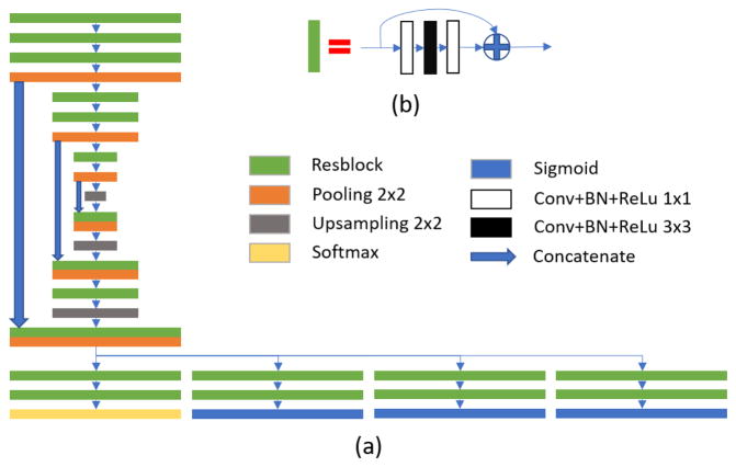
FCN has been applied for semantic segmentation in computer vision and has achieved promising results. FCN trains the end-to-end neural networks for pixel- or voxel-wise segmentation. In the FCN architecture, the feature learning stage and the segmentation (or classification) stage are combined into the same network, and their network parameters can be optimized at the same time. However, it is often difficult to optimize a large number of parameters, because of gradient vanishing problem caused by the deep architecture. In this paper, we use the idea from residual learning, which can effectively alleviate the gradient vanishing problem and make the training faster. The residual learning block is shown in Fig. 1(b), and the residual function to be learned can be formulated as follows:

$$y=F(x,W)+x$$ (1)

where x and y are the input and output of residual learning block, and W denotes parameters in the block.

Fig. 1.

(a) Architecture of proposed networks; (b) residual learning block.

In the FCN architecture, segmentation maps are obtained by upsampling the low-resolution feature maps. Thus, some low-level information does not involve in the final segmentation. In order to use low-level information effectively, concatenation-based skip connection is employed to connect low-level feature maps with the same-sized high-level feature maps, as shown in Fig. 1(a). After concatenation, a series of convolution operations and upsampling operation are applied to generate higher-level feature maps. And the obtained feature maps are concatenated with lower-level feature maps as well.

After feature learning with residual FCN, the feature maps are sent to four tasks, which include three regression tasks (for estimating the intensity maps of bladder, prostate and rectum, respectively) and one segmentation task (for segmenting the bladder, prostate and rectum jointly). The parameters in feature learning are optimized by all four tasks. This multi-task learning strategy is explained in detail below.

2.1.2. Multi-task learning

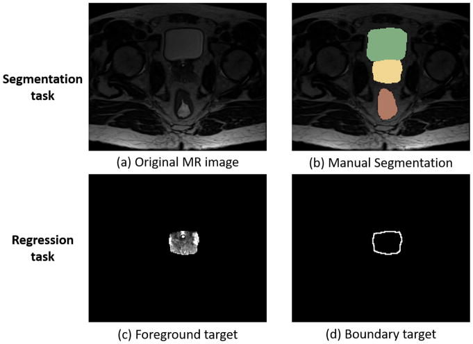
In the single task situation, segmentation task usually applies a softmax function to activate the top layer and to output four probability maps (for segmenting bladder, rectum, prostate and background). However, the segmentation results are sometimes inaccurate on the boundary of organs with low contrast. To address this problem, three regression tasks with their respective sigmoid activated top layers are also employed to predict foreground and boundary for each of three organs (bladder, rectum and prostate). Information learned from the regression tasks can guide the segmentation in the low contrast regions. It is worth noting that each regression task includes two target maps, i.e., the original intensity and boundary maps of an organ, as shown in Fig. 2(c)(d) by using prostate as example.

Fig. 2.

(a)(b) A pelvic MR image and its corresponding labels of the manually-segmented bladder (green), prostate (yellow), rectum (red). (c)(d) Target maps (normalized to the range of [0,1]) in a regression task for the prostate.

2.1.3. Loss function

The size of each organ under segmentation is quite different, which could make small organs less focused during segmentation. To overcome this problem, we provide different weights to different organs in the definition of the overall loss function. Specifically, for the segmentation task, we used a weighted cross-entropy loss as below:

$$Ls({\theta }_s)=-\sum _j\sum _{i=0}^3{w}^{(i)}{Y}_j^{(i)}log{y}_j^{(i)}$$ (2)

where s denotes segmentation task, w⁽ⁱ⁾ is the weight for organ i (0 for background), Y_j and y_j are the label and the probability (predicted by network parameters θ_s) at voxel j. For each of three regression tasks, the square error loss function is adopted:

$$L{r}_i({\theta }_f,{\theta }_b)=-\sum _j{(Z_{f,j}^{(i)}-z_{f,j}^{(i)})}^2+{\lambda }^{(i)}{(Z_{b,j}^{(i)}-z_{b,j}^{(i)})}^2$$ (3)

where r denotes regression tasks, Z and z are the target and predicted intensities, λ is the weight of organ for boundary target map, f and b denote foreground and boundary regression, respectively. Note that the weight of boundary λ is inversely proportional to the number of voxels in the target map.

Finally, the overall loss function of the networks can be described as Eq. (4):

$$L(\theta )=Ls+\sum _{i=1}^3{\rho }_{i}L{r}_i$$ (4)

where Ls is the segmentation loss, and Lr_i is the regression loss of organ i. Similar with the definition of segmentation loss, different weights ρ are also given to the three regression tasks for three organs. In this work, we set ρ₁ = 0.15 (for bladder), ρ₂ = 0.5 (for prostate), ρ₃ = 0.35 (for rectum).

2.2. Semi-supervised learning

In the supervised learning stage, we train the network θ on the training set L = {I,S}, which consists of N MR images I = {I₁, I₂, …, I_N} and their corresponding segmentation maps S = {S₁, S₂, …, S_N}. In the semi-supervised stage, we have an unlabeled data set U = {I_U}, and then build a semi-supervised learning algorithm, with the inputs of θ, L, U and the output of updated θ, to progressively train the network with unlabeled data. The basic steps of our proposed semi-supervised learning algorithm are provided in Algorithm 1, where the best k pairs of unlabeled data with reasonable segmentations are included into the training set at each progressive refinement iteration.

As shown in Algorithm 1, the training set is enlarged by including some reasonable segmentations of unlabeled data in each iterative step. The expansion of the training set L and also the update of parameters θ alternately proceed. Note that, given the updated training set, the training of the networks is the same as in the supervised stage.

Algorithm 1.

Progressive Semi-supervised Learning

Input: θ, L, U
Output: updated θ
1:	while len(U) > 0 do
2:	Estimate SU by θ
3:	Move k best pairs (IU, SU) from U to L
4:	Optimize θ by training on L
5:	return θ

2.3. Training

Our proposed method is implemented using keras¹. The network parameters are initialized by Xavier algorithm [11], which determines the scale of initialization based on the numbers of neurons. The network parameters are updated by the back-propagation algorithm using Adam optimizer [12], and the parameters are lr = 0.0001, β₁ = 0.9, β₂ = 0.999. The intensities of all images are normalized to the range of [0,1] and further cropped to the size of 168×112×5 as the input of the network. GTX1080 Ti GPU is used to train the networks.

3. EXPERIMENTS AND RESULTS

In the experiments, we adopt Dice ratio as a metric to evaluate the segmentation performance of the three organs (bladder, prostate and rectum) by using 30 subjects for training and 10 subjects for testing. In addition, other 30 unlabeled data are also used for semi-supervised learning. The three organs for all MR images in the training and testing sets have been manually labeled by a physician, which are used as the ground truth for validating our segmentation method. The original image size is mostly 256×256×X(120 ~ 176), with image resolution 1.0 × 1.0 × 1.0 mm³.

3.1. Impact of multi-task learning

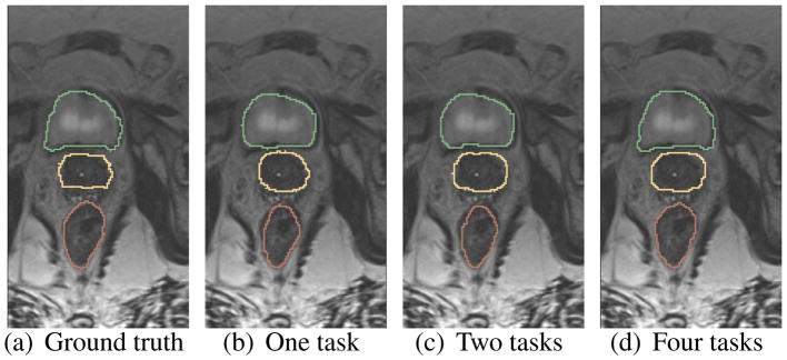
As mentioned in Sec. 2.1.2, the networks are optimized by the four tasks. To investigate the impact of multi-task learning, we train our networks with different task settings: 1) with only one task (i.e., segmentation), 2) with two tasks (i.e., segmentation and prostate/bladder/rectum regression), and 3) with all four tasks (i.e., segmentation, prostate regression, bladder regression and rectum regression). Note that the segmentation results by our networks are refined by morphological operations [13]. The Dice ratios of segmentation for the above three different cases are shown in Table 1. It can be seen that, by including a regression task, the second case of using two tasks can segment each organ better than the first case of using one task. And, our proposed networks (i.e., the third case of using four tasks) work the best on segmentation of all three organs. The segmentation maps of different task settings are also shown in Fig. 3.

Table 1.

Comparison of single- and multi-task learning networks. The bold denotes the best performance for each organ, in terms of Dice ratio (standard deviation).

	Bladder	Prostate	Rectum
one task	.935(.015)	.877(.031)	.868(.034)
two tasks	.938(.016)	.889(.021)	.869(.033)
four tasks	.952(.007)	.891(.019)	.884(.027)

Fig. 3.

Comparison of the segmentation results of single-task networks and multi-task networks.

3.2. Impact of semi-supervised learning

In Sec. 2.2, we have introduced a progressive semi-supervised learning algorithm. In order to evaluate its impact, we have compared it with the supervised learning as well as the conventional semi-supervised algorithm, which iteratively fine-tunes the networks with all predicted segmentation maps of all unlabeled data.

The network parameters are similarly initialized by the same training set with 30 labeled MR images, and then refined by other 30 unlabeled MR images with different semi-supervised learning methods. The parameter k in Algorithm 1 is set to 5, and the alternate updating in the conventional semi-supervised learning algorithm is performed for 6 iterations. The performances of three algorithms are shown in Table 2. The results show that, using our proposed semi-supervised learning to enlarge the training data could better improve the segmentation performance. Also, progressively including the unlabeled data into the training set for updating the network parameters can perform better than the conventional semi-supervised learning.

Table 2.

Comparison of supervised learning, conventional learning, and proposed semi-supervised learning. The bold denotes the best performance for each organ.

	Bladder	Prostate	Rectum
Supervised	.952(.007)	.891(.019)	.884(.027)
Conventional learning	.960(.006)	.895(.024)	.884(.031)
Proposed learning	.963(.007)	.903(.022)	.890(.029)

4. CONCLUSION

In this paper, we proposed a multi-task residual FCN based semi-supervised framework to segment pelvic organs from MR images. The network was trained in an end-to-end and voxel-to-voxel fashion to achieve segmentation map. The multi-task design was able to effectively provide information from regression tasks to improve the segmentation performance. Also, experimental results showed that the proposed progressive semi-supervised learning strategy could effectively use unlabeled data to help train the networks.

References

- 1.Liao Shu, et al. Automatic prostate mr image segmentation with sparse label propagation and domain-specific manifold regularization. IPMI. 2013;23:511. doi: 10.1007/978-3-642-38868-2_43. [DOI] [PMC free article] [PubMed] [Google Scholar]
- 2.Toth Robert, et al. Accurate prostate volume estimation using multifeature active shape models on t2-weighted mri. Academic radiology. 2011;18(6):745. doi: 10.1016/j.acra.2011.01.016. [DOI] [PubMed] [Google Scholar]
- 3.Ghose Soumya, et al. A random forest based classification approach to prostate segmentation in mri. MICCAI Grand Challenge: PROMISE12. 2012;2012 [Google Scholar]
- 4.Liu Manhua, et al. Tree-guided sparse coding for brain disease classification. MICCAI. 2012:239–247. doi: 10.1007/978-3-642-33454-2_30. [DOI] [PMC free article] [PubMed] [Google Scholar]
- 5.Yang Meijuan, et al. Prostate segmentation in mr images using discriminant boundary features. IEEE TBE. 2013;60(2):479–488. doi: 10.1109/TBME.2012.2228644. [DOI] [PMC free article] [PubMed] [Google Scholar]
- 6.Guo Yanrong, et al. Deformable mr prostate segmentation via deep feature learning and sparse patch matching. IEEE TMI. 2016;35(4):1077–1089. doi: 10.1109/TMI.2015.2508280. [DOI] [PMC free article] [PubMed] [Google Scholar]
- 7.Nie Dong, et al. ISBI. IEEE; 2016. Fully convolutional networks for multi-modality isointense infant brain image segmentation; pp. 1342–1345. [DOI] [PMC free article] [PubMed] [Google Scholar]
- 8.Long Jonathan, et al. Fully convolutional networks for semantic segmentation. CVPR. 2015:3431. doi: 10.1109/TPAMI.2016.2572683. [DOI] [PubMed] [Google Scholar]
- 9.He Kaiming, et al. Deep residual learning for image recognition. CVPR. 2016:770–778. [Google Scholar]
- 10.Evgeniou Theodoros, et al. Regularized multi–task learning. SIGKDD. 2004:109. [Google Scholar]
- 11.Glorot Xavier, et al. Understanding the difficulty of training deep feedforward neural networks. AISTATS. 2010:249–256. [Google Scholar]
- 12.Kingma Diederik, et al. Adam: A method for stochastic optimization. 2014 arXiv preprint arXiv:1412.6980. [Google Scholar]
- 13.Chen Su, et al. Recursive erosion, dilation, opening, and closing transforms. TIP. 1995;4(3):335. doi: 10.1109/83.366481. [DOI] [PubMed] [Google Scholar]