Pairwise and higher order genetic interactions during the evolution of a tRNA

Summary

A central question in genetics and evolution is the extent to which mutations have outcomes that change depending on the genetic context in which they occur^1–3. Pairwise interactions between mutations have been systematically mapped within^4–18 and between¹⁹ genes, and contribute substantially to phenotypic variation amongst individuals²⁰. However, the extent to which genetic interactions themselves are stable or dynamic across genotypes is unclear^21,22. Here we quantify >45,000 genetic interactions between the same 87 pairs of mutations across >500 closely related genotypes of a yeast tRNA. Strikingly, all pairs of mutations interacted in at least 9% of genetic backgrounds and all pairs switched from interacting positively to interacting negatively in different genotypes (FDR<0.1). Higher order interactions are also abundant and dynamic across genotypes. The epistasis in this molecule means that all individual mutations switch from detrimental to beneficial in even closely-related genotypes. As a consequence, accurate genetic prediction requires mutation effects to be measured across different genetic backgrounds and the use of higher order epistatic terms.

Genetic (epistatic) interactions have been extensively mapped between pairs of mutations within individual genes^4–18, and also between individual alleles of many different genes¹⁹. However, the pairwise mapping of interactions only provides a limited view of genotype space, which has a vast combinatorial size²². Genetic interactions between genes have been reported as only poorly or moderately conserved between species²¹. Moreover, analyses of the effects of combinations of mutations within individual genes has pointed to the importance of higher order epistasis^22–25, in which mutations interact beyond pairwise interactions to determine mutation effect.

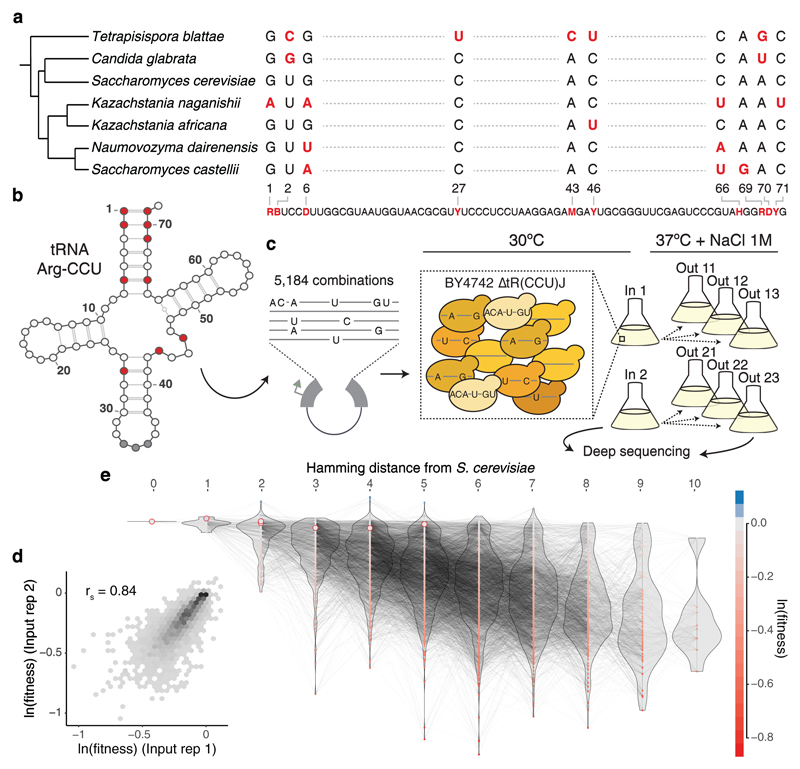
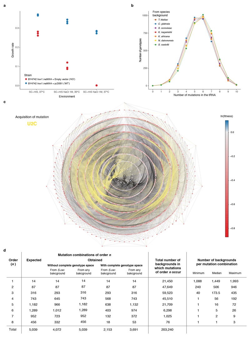
To directly test the extent to which the effects of mutations and the interactions between mutations are stable or change depending upon the genotype on which they occur, we designed an experiment in which mutation effects and interactions are quantified across a large number of closely-related genetic backgrounds. As a model system, we used a single copy Arginine-CCU tRNA gene that is conditionally required for the growth of budding yeast (Extended Data Fig. 1a) and for which pairwise interactions have been previously mapped in one genetic background¹⁵. The small size of the gene allowed us to design a library that covered all 5,184 (= 2⁶ x 3⁴) genotypes containing the 14 nucleotide substitutions observed in ten positions in post-whole genome duplication yeast species²⁶ (Fig. 1a, b). Each genotype therefore varies from zero to a maximum of ten nucleotides divergence from the Saccharomyces cerevisiae tRNA sequence (Extended Data Fig. 1b). Following transformation of the library into S. cerevisiae, we performed six parallel selection experiments to quantify the relative fitness of each of the 5,184 variants in the restrictive conditions of high temperature and 1M NaCl (Fig. 1c). The fitness of each genotype was quantified as the change in its abundance in each culture between the beginning and end of the competition by deep sequencing using a hierarchical error model and normalised in log scale to the fitness of the S. cerevisiae genotype (henceforth ‘fitness’, see Methods). After filtering, we obtained fitness measurements for 4,176 variants (Supplementary Table 1) that correlated well across replicates (Fig. 1d). The median fitness declines as the number of mutations increases but there are still many combinations of mutations with high fitness amongst genotypes far from the reference genotype (Fig. 1e).

Figure 1. Combinatorially-complete fitness landscape of a tRNA.

a, Species phylogenetic tree²⁶ and multiple sequence alignment of the tRNA-Arg-CCU orthologs. Shown variable positions across the seven yeast species with the synthesized library below. R - A or G, B - C, G or T, D - A, G or T, Y - C or T, M- A or C, H - A, C or T. b, Secondary structure of S. cerevisiae tRNA-Arg-CCU (varied positions in red). c, Selection experiment and structure of the replicates. From each independent yeast transformation (input) three independent selection experiments were performed. d, Correlation between weighted-averaged input replicates (r_s = Spearman correlation coefficient, n = 4,176 genotypes). e, Fitness landscape of the tRNA-Arg-CCU genotipes (nodes). Colour indicates ln(fitness) relative to the S. cerevisiae tRNA. Edges connect genotypes differing by a single substitution. Genotypes and distribution of fitness values (violins) are arranged in the x-axis according to the total number of substitutions from the S. cerevisiae tRNA. Highlighted nodes indicate the genotypes of the seven extant species.

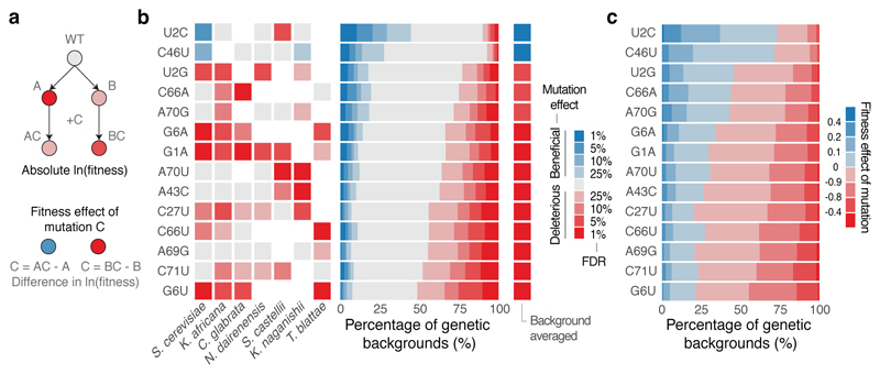
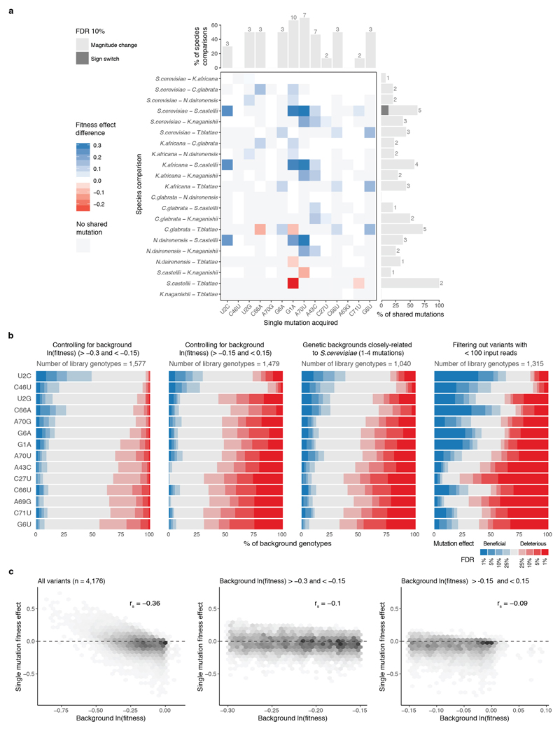
We first examined the fitness consequences of single mutations and how these change across different genetic backgrounds (Fig. 2a). In the S. cerevisiae genotype, six of the 14 individual mutations were detrimental (Fig. 2b). However, when the same 14 mutations were made in the tRNA genotypes of the other six extant species (these alternative ‘wild-type’ tRNAs have fitness very close to the S. cerevisiae tRNA when expressed in S. cerevisiae, Supplementary Table 2), their effects changed substantially (Fig. 2b). For example, the mutation C66A had no effect in the S. cerevisiae background but became detrimental in the Candida glabrata tRNA, which only differs by two substitutions (paired t-test q-val = 0.006, n = 6). Indeed, 11/14 mutations had effects that changed across these seven tRNAs from different species (Extended Data Fig. 2a, FDR<0.1).

Figure 2. All single mutations switch sign from detrimental to beneficial in different genetic backgrounds.

a, The same mutation can have different fitness consequences depending on the genetic background. b, Significance of beneficial (blue) or detrimental (red) mutation effects in the backgrounds of each species (left) and across all genetic backgrounds (right). FDR = False Discovery Rate, n = 21,450 backgrounds, see Methods). c, Proportion of genetic backgrounds in which each mutation has beneficial (blue) or detrimental (red) effects.

We next compared the effects of the single mutations across the complete set of genetic backgrounds in the library. In total, we tested each mutation in a median of 1,449 genetic backgrounds (min = 1,088, max = 1,993, Extended Data Fig. 1c, d). Surprisingly, we found that every mutation was both detrimental and beneficial in a substantial number of genetic backgrounds (Fig. 2b, c, median number of backgrounds in which the less frequent sign was observed = 6.4%; min = 3.4%; max = 11.9% across all 14 mutations, FDR<0.1, n = 21,450, See Methods). Restricting the analyses to background genotypes with high or intermediate fitness, to genotypes with high input read counts, or to genotypes with few mutations did not change this conclusion (Extended Data Fig. 2b). Thus, all mutations have effects that switch from beneficial to detrimental in closely related genotypes.

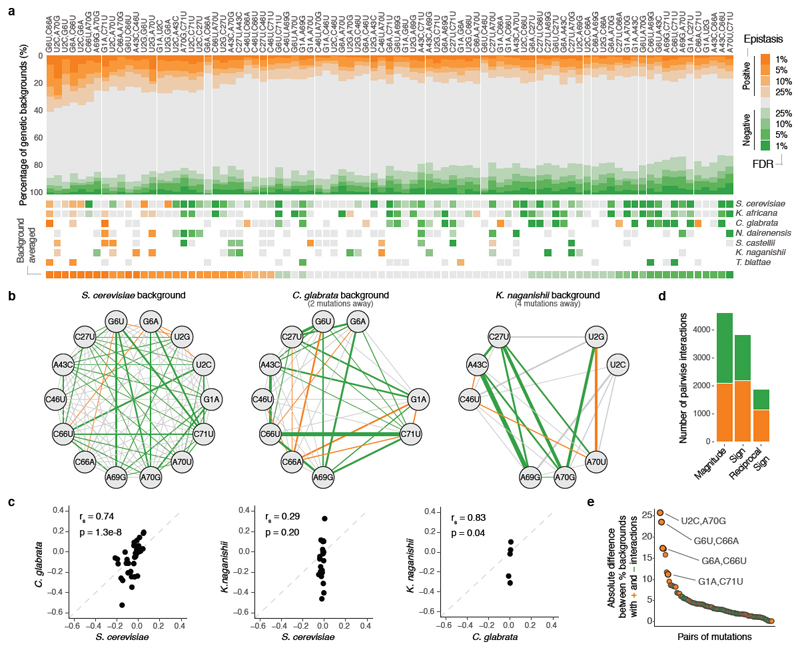
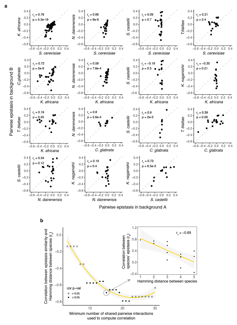
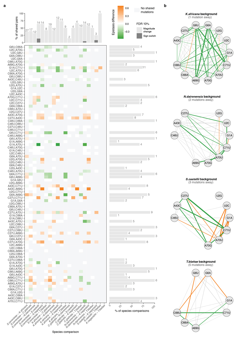
To investigate the interactions between mutations that underlie these changes in mutation effects, we first quantified pairwise genetic interactions between the 14 mutations, which is a total of 87 pairs in any genotype. We define epistasis as the difference between the fitness of each double mutant and the sum of the fitness of the two corresponding individual mutations. Consistent with previous results¹⁵, in the S. cerevisiae genotype, many pairs of mutations (40.2%, 35/87) had combined fitness effects that were more detrimental than expected (negative epistasis) and only a few had effects that were less detrimental than expected (positive epistasis, 5.7%, 5/87, FDR<0.1, Fig. 3a). However, these interactions changed when they were tested in the tRNAs from the different species (Fig. 3b, c, Extended Data Fig. 3), with 83/87 interactions differing across the species (n = 1,000 paired t-tests, FDR<0.1, Extended Data Fig. 4).

Figure 3. Genetic interactions between all pairs of mutations switch from positive to negative epistasis in different genetic backgrounds.

a, Proportion of backgrounds (top) and species (middle) in which each pair of mutations interacts positively (orange) negatively (green) at different FDRs (n = 47,649 backgrounds). Bottom shown background-averaged epistasis (n = 87 pairs of mutations). b, Interaction networks for three species (other species in Extended Data Fig. 4b). Edge colours indicate epistasis sign (FDR<0.1) and width strength of interaction. c, Comparison of epistasis scores between these three species (r_s = Spearman correlation coefficient, n = 43, 22 and 6 comparisons from left to right). d, Number of positive (orange) or negative (green) magnitude, sign or reciprocal sign pairwise epistasis (n = 10,330 significant interactions from 47,649 tested) e, Consistency of each interaction quantified as the absolute difference between the % of backgrounds in which the interaction is positive or negative. Colour indicates the predominant sign. The four pairs that restore WC bps are highlighted.

We next analysed how the 87 interactions changed across all the genetic backgrounds in the library. Each interaction was quantified in a median of 506 genetic backgrounds (min = 240, max = 946, Extended Data Fig. 1d). Strikingly, all 87 interactions switched from positive to negative in a substantial proportion of the genetic backgrounds (Fig. 3a). Restricting our analyses to genetic backgrounds with high or intermediate fitness, to combinations with high expected fitness, or to genotypes with high input read counts did not change this conclusion (Extended Data Fig. 5b). Across all genetic backgrounds, positive and negative interactions were similarly prevalent (11.4% and 10.3% for positive and negative epistasis respectively, FDR<0.1, n = 47,649, see Methods).

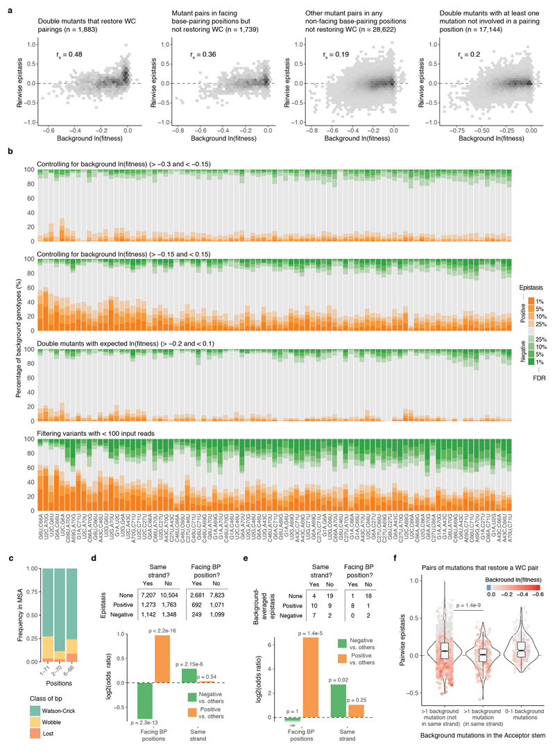
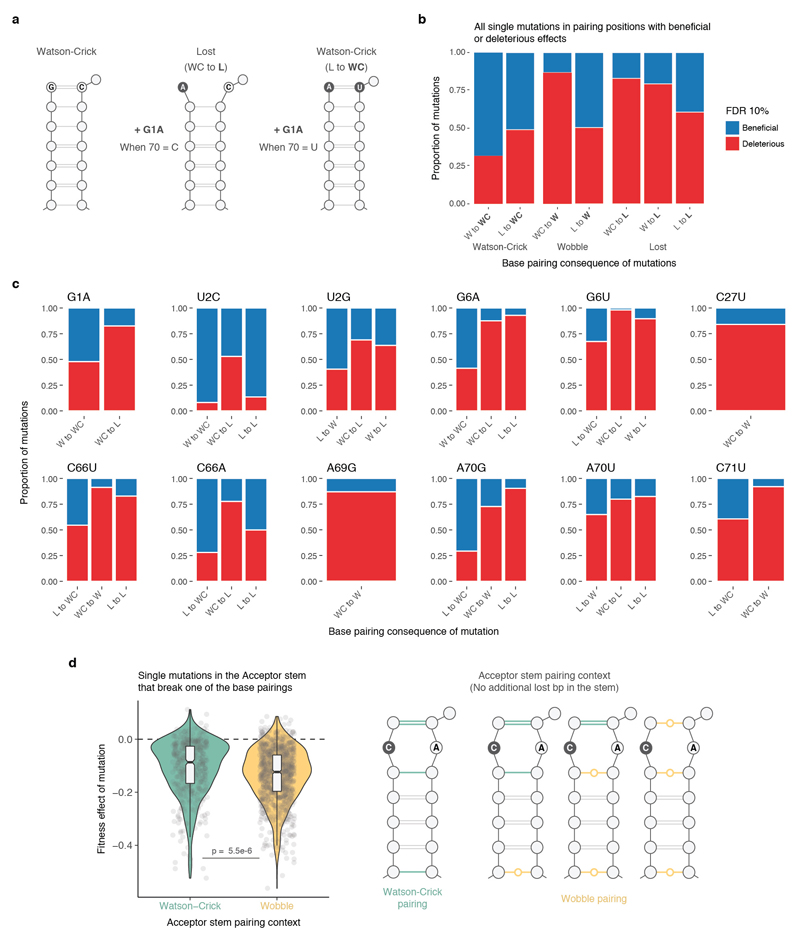
Changes in base pairing only partially explained changes in sign and magnitude of single mutations (Extended Data Fig. 6). The four pairs of mutations that restore Watson-Crick base pairs (WC bps) were amongst the most robust positive interactions (Fig. 3e). However, even these combinations interacted negatively in a large fraction of backgrounds (5.9-8.4%). This is consistent with the presence of non WC bp nucleotides in these positions in the tRNAs from other species²⁷ (Extended Data Fig. 5c). Double mutants in the same RNA strand of the acceptor stem were enriched for negative epistasis (OR = 1.23, p-value = 2.15e-6, Extended Data Fig. 5d-e) and the restoration of a WC bp was also more likely to result in a negative interaction when the stem harboured multiple additional mutations in a single strand (Extended Data Fig. 5f). This suggests that other mechanisms, for example stacking interactions, are also important determinants of tRNA function.

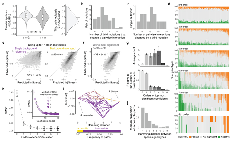
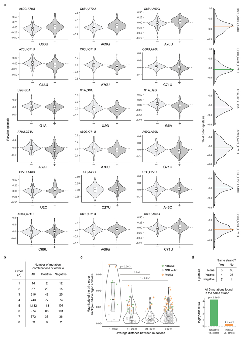
We next tested whether pairwise interactions changed in backgrounds containing each additional single mutation (Fig 4a, Extended Data Fig 7a). Strikingly, 76/87 interactions were significantly altered by the presence of a single additional mutation in the background (Fig. 4b), constituting a total of 138/316 possible third order interactions when averaging across genetic backgrounds (Extended Data Fig 7b, FDR<0.1). All 14 individual mutations altered at least eight pairwise interactions (median = 16.5, max = 24, Fig. 4c). Third order interactions, as second order, were enriched amongst proximal mutations and mutations found in the same strand (Extended Data Fig. 7c, d).

Figure 4. Averaging coefficients across genetic backgrounds and using higher order epistatic terms is important for genetic prediction.

a, Changes in the distribution of pairwise epistasis when the genetic backgrounds contain or not the indicated mutation (left) and distribution of the corresponding third order epistasis values (right). b, Distribution of pairwise interactions altered by a third mutation. c, Distribution of single mutations involved in a third order interaction. d, Proportion of genetic backgrounds in which each combination of mutations from 3^rd to 8^th order interact positively (orange) or negatively (green) at a FDR<0.1. e, Agreement between observed and predicted fitness values of all 8^th order complete sub-landscapes (n = 19,456 genotypes, 76 sub-landscape with 256 genotypes each) when using up to 1^st order epistatic coefficients, relative to a single background genotype (left) or averaged across backgrounds (right, 10-fold cross-validation). %VE = Percentage of variance explained. f, Agreement between observed and predicted fitness values for all complete 8^th order sub-landscapes when using the most significant epistatic coefficients, estimated by 10-fold cross-validation. g, Mean root-mean-square error (RMSE) across the 76 8^th order sub-landscapes when cumulatively adding most significant coefficients determined by cross-validation (right, colour indicates de median order of the coefficient added across 76 sub-landscapes) or all significant coefficients from the same order (left). Error bars are 95% CI. h, Mean orders of most significant epistatic coefficients (top, absolute counts; bottom, relative to the possible number of coefficients per order). Error bars are 95% CI. i, Example of shortest paths between two extant species (top) and accessible proportion (bottom). j, Average frequency of accessible paths between species.

However, as for pairwise interactions, all third order interactions (316/316) also switched from positive to negative across different genetic background, indicating the presence of higher order epistasis (Fig. 4d). 260/316 third order interactions changed in the presence of a fourth mutation (FDR<0.1, n = 740). Indeed, interactions can be detected in this dataset up to the eighth order (Extended Data Fig. 7b, a total of 763 background-averaged epistatic interactions from 3,961 possible interactions tested from order one to eight, FDR<0.1). Consistent with the behaviour of the lower order interactions, the signs of many higher order interactions also switch from positive to negative as the genetic background changes (Fig. 4d, 1,981/3,691 interactions in the total dataset interact both positively and negatively in different genetic backgrounds, FDR<0.1).

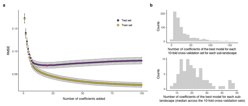
Finally, we evaluated the extent to which epistasis affected our ability to predict phenotypes from genotypes. We quantified the accuracy of genetic prediction in the 76 complete di-allelic sub-landscapes of eight mutations using models restricted to a single genetic background as a reference or after averaging epistatic terms across backgrounds (See Methods). While individual mutations effects quantified in a single genetic background provide quite poor prediction (Fig. 4e, percentage of variance explained %VE = -22%), the average effect of each mutation across all genotypes within a sub-landscape improves the prediction (Fig. 4e, %VE = 58% on held-out data, 10-fold cross-validation). The most significant coefficients selected by the cross-validated models (Extended Data Fig.4a, See methods) explained 64% of the fitness variance across all complete di-allelic sub-landscapes of eight mutations (Fig. 4f). The best predictive models contained not only first and second order but also higher order interaction terms (Fig. 4 g) that progressively improved the models’ predictive performance (Fig. 4h). However, these models contained a relatively small number of coefficients (20/256 coefficients on average across sub-landscapes, Extended Data Fig. 8b), suggesting that although pairwise and higher order epistasis is important, reasonably sparse models can provide good genetic predictions when coefficients are measured across different genetic backgrounds.

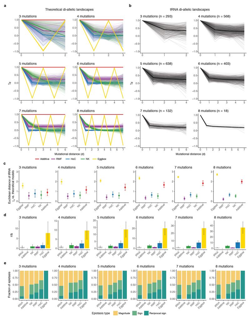
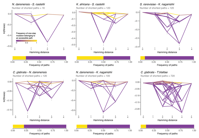
Taken together, our results show even single steps in sequence space substantially change the effects of both individual mutations and how they combine to alter fitness. By a range of metrics, the combinatorially-complete tRNA fitness sub-landscapes are most similar to rugged theoretical fitness landscapes²⁸ that constrain evolution (Extended Data Fig. 9). Indeed, the abundance of sign epistasis (Fig. 3d) limits the number of accessible evolutionary paths²⁹, for example between the genotypes of extant species (Fig. 4i, j, Extended Data Fig. 10). These results add to a growing body of evidence² that evolution is highly contingent at the molecular level. As a consequence, models that that use coefficients averaged across different genetic backgrounds and that incorporate higher order epistatic terms provide more accurate genetic prediction.

Methods

1. Library design

tRNAs orthologous to S. cerevisiae Arginine tRNA CCU (HSX1) were collected from the Genomic tRNA Database³⁰ or extracted from each specie’s genome using Blast³¹ (‘blastall’ 2.2.25). The sequences were aligned with Clustal Omega³². Across the 12 species closest to S. cerevisiae, only the six species shown in Fig. 1a had substitutions in the gene, with a total of 14 substitutions in ten positions. Allowing all of these substitutions to co-occur results in a total library size of 5,184 (= 2⁶ x 3⁴) possible mutation combinations.

2. Plasmid library construction

A 115 nt long oligonucleotide containing 72 nt of tRNA flanked by 21 and 22 nt of the yeast endogenous promoter and terminator was synthesised by IBA Lifesciences. At ten of the 72 positions of the tRNA, two or three different nucleotides were mixed in equal proportions during synthesis. For example, position 1 can be G or A, but position 2 can be T, G or C.

The oligonucleotide was amplified by PCR for 10 cycles (Q5 Hot Start High-Fidelity DNA Polymerase, NEB), purified using an E-gel electrophoresis system (E-Gel SizeSelect Agarose Gel 2%) followed by column purification (MinElute PCR Purification Kit, Qiagen). Subsequently, the purified oligo was cloned into a version of the yeast centromeric plasmid pRS413 (HIS3 marker)³³ that contained the HSX1 gene flanked by its 218 bp upstream and 202bp downstream genomic sequences (pJD001). pJD001 was linearized from the HSX1 flanking regions (excluding the HSX1 sequence) by PCR (Q5 Hot Start High-Fidelity DNA Polymerase, NEB) and later purified by gel extraction (QIAquick Gel Extraction Kit, Qiagen). The library of oligos was cloned into 400 µg of linearised pJD001 substituting the ‘wt’ HSX1 gene by Gibson reaction (prepared in house) at 50ºC for 12 h with a ratio 5:1 of insert:vector. After dialyzing the reaction with 0.025 µm VSWP membrane filters (Merck Millipore) for 1.5 h, the product was concentrated 4X by speed-vac. 6 µL of the concentrated reaction were transformed into 100 µl of electrocompetent E. coli (NEB® 10-beta Electrocompetent E. coli, NEB) according to the manufacturer’s protocol. Cells were allowed to recover in SOC (NEB® 10-beta/Stable Outgrowth Medium) for 30 min and later transferred to 150mL of LB medium with Ampicillin 4X overnight. A total of ~9.59x10⁶ transformants were estimated. Given the complexity of the library, each variant was therefore represented ~1,849 times on average. 50 mL of E. coli saturated culture was harvested to extract the plasmid library by plasmid midi prep (QIAfilter Plasmid Midi Kit, Qiagen).

3. Selection experiment

3.1. Yeast strain and conditional growth defect in different environmental conditions

The HSX1 deletion strain was obtained by replacing the HSX1 gene with a Nourseothricin resistance cassette in the haploid laboratory strain BY4742 (MATα his3Δ1 leu2Δ0 lys2Δ0 ura3Δ0 hsx1::natMX4) and later confirmed by colony PCR. The deletion of the single copy Arginine tRNA CCU (HSX1) in yeast was previously reported to lead to a conditional growth defect when the temperature is raised from 30ºC to 37ºC15. We found that a similar growth defect is observed if the growth medium contains high salt concentrations (1M NaCl), and that a combination of high temperature and high salt gives an even stronger defect (Extended Data Fig. 1a). SC-HIS 1M NaCl at 37ºC was therefore used as the selective condition for the library selection experiment.

3.2. Large-scale yeast transformation

The high-efficiency yeast transformation protocol was derived from Melamed et al.⁷. Two pre-cultures of the tRNA deletion strain were grown independently in 25 mL standard YPDA at 30ºC overnight. The next morning, the cultures were diluted into 175 mL of fresh YPDA at an OD_600nm = 0.3. The two cultures were incubated at 30ºC for 4 h (~2-3 generations). After growth, the cells were harvested and centrifuged for 5 min at 3,000g, washed in sterile water and later in SORB (100mM LiOAc, 10mM Tris pH 8.0, 1mM EDTA, 1M sorbitol). The cells were re-suspended in 8.6 mL of SORB and incubated at room temperature for 30 min. After incubation, 175 µL of 10mg/mL boiled salmon sperm DNA (Agilent Genomics) was added to each tube of cells, as well as 3.5 µg of plasmid library. After 10 min of gentle shaking at room temperature, 35 mL of Plate Mixture (100mM LiOAc, 10mM Tris-HCl pH 8, 1mM EDTA/NaOH, pH 8, 40% PEG3350) were added to the cells and incubated at room temperature for 30 more min. 3.5 ml of DMSO was added to each tube and the cells were then heat shocked at 42ºC for 20 min (inverting tubes from time to time to ensure homogenous heat transfer). After heat shock, each independent tube of cells was centrifuged and re-suspended in 350 mL of YPD + 0.5M Sorbitol and allowed to recover for 1h at 30ºC. The cells were then centrifuged, washed twice with SC-HIS medium and re-suspended in 350 mL SC-HIS. The two independent transformations were grown at 30ºC for ~60 h until saturation. For the two independent transformations, 1.5x10⁶ and 1.1x10⁶ transformants were obtained, which ensured that each variant of the library was on average represented ~250 times³⁴.

3.3. Competition assay

The competition experiment had two different phases. In phase one, the environment had minimal selection on the tRNA functionality (SC-HIS at 30ºC), allowing the pool of variants to be amplified and the cells to enter the exponential growth phase (input library)³⁴. In the second stage, the medium was changed to a condition (SC-HIS 1M NaCl medium at 37ºC) where non-functional tRNA variants would lead to a severe growth defect phenotype (output library). The assay was performed immediately after yeast transformation to avoid recovering cells from frozen glycerol stocks. Once the two independently transformed cultures reached saturation (~60 h after plasmid transformation), they were inoculated at an OD_600nm of 0.08 in 500 mL of SC-HIS medium and grown for 4 generations at 30ºC (~11 h). When exponential phase was reached after 4 generations of growth, the cells were harvested and washed with selection medium (warm SC-HIS NaCl 1M) and then inoculated in 500 ml of selection medium at OD_600nm 0.015. The remainder of the cells was harvested and stored at -20ºC for later DNA extraction of the input libraries. Each independent input library was divided into three different output libraries (six replicates in total). Cells were grown in selective conditions for ~6.5 generations (~26.5 h). This number of generations was chosen so that null alleles, which grow ~0.18 generations every 3 h, would be detected after sequencing with an average read coverage of ~150 reads per variant. After 6.5 generations, the cells were harvested and the cell pellets stored at -20ºC for later DNA extraction of the output libraries.

3.4. DNA extraction and quantification

Cell pellets (eight tubes, two inputs and six outputs) were re-suspended in 1.5 mL extraction buffer (2% Triton-X, 1% SDS, 100mM NaCl, 10mM Tris-HCl pH8, 1mM EDTA pH8), frozen by dry ice-ethanol bath and incubated at 62ºC water bath twice. Subsequently, 1.5 mL of Phenol/Chloro/Isoamyl 25:24:1 (equilibrated in 10mM Tris-HCl, 1mM EDTA, pH8) was added, together with 1.5 g of glass beads and the samples were vortexed for 10 min. Samples were centrifuged at RT for 30 min at 4,000 rpm and the aqueous phase was transferred into new tubes. The same step was repeated twice. 0.15 mL of NaOAc 3M and 3.3 mL of cold ethanol 100% were added to the aqueous phase. The mix was incubated at -20ºC for 30 min and after that, centrifuged for 30 min at full speed at 4ºC to precipitate the DNA. The ethanol was removed and the DNA pellet allowed to dry overnight at RT. DNA pellets were re-suspended in 900 µL TE 1X and treated with RNaseA (10mg/mL, Thermo Scientific) for 30 min at 37ºC. To desalt and concentrate the DNA solutions, QIAEX II Gel Extraction Kit was used (75 µL of QIagen beads). The samples were washed 3 times with PE buffer and eluted twice in 375 µL of 10 mM Tris·Cl buffer, pH 8.5.

3.5. Sequencing library preparation

The plasmid concentration in each total DNA sample was quantified in triplicate by real time quantitative PCR, using primers that had homology to the origin of replication region of the pJD001 plasmid backbone (Supplementary Table 3). On average, we obtained ~3.5 x10⁶ plasmid molecules per µL of DNA sample.

A 2-step PCR using high fidelity Q5 Hot Start High-Fidelity DNA Polymerase (NEB) was used to amplify the input and output libraries for sequencing. In each sample, ~30 million plasmid molecules were amplified for 10 cycles using primers with overhang homology to Illumina sequencing adapters (Supplementary Table 3). The first PCR reaction was performed independently for each of the eight samples. The samples were then treated with ExoSAP (Affymetrix) and cleaned by bead purification with a QIAEX II kit. The whole eluates, corresponding to the entire first PCR reactions, were used for the second PCR reactions (15 cycles), where the rest of the Illumina adapter was added as overhangs on the primers, in addition to sample-specific indexes. The DNA concentration of each individual second PCR was quantified by fluorometric quantitation (Quant-iT™ PicoGreen® dsDNA Assay Kit) and pooled together at an equimolar ratio. finally, the pooled sequencing library was gel purified (QIAEX II Gel Extraction Kit) and subjected to 125 bp paired-end sequencing on an Illumina HiSeq 2500v5 sequencer at the EMBL Genomics Core Facility (Heidelberg, Germany).

4. Data analysis

4.1. From sequencing reads to fitness values

The sequencing reads of each sample (two inputs and six outputs) were processed and filtered independently. Each sequencing read covered the entire tRNA. The 5’ and 3’ constant regions of the read (primers annealing sites) were removed with the ‘cutadapt’ software³⁵. The forward and reverse reads were merged using PEAR³⁶ and sequences that were either not assembled due to low quality or unexpected length were discarded. Unique genotypes were called and quantified with custom python scripts. Genotypes with less than nine input reads in any input replicate, unexpected nucleotide substitutions (sequencing or PCR errors) or zero reads in the outputs were discarded. After filtering, we ended up with a total of 4,176 sequence genotypes quantified in all inputs and outputs.

To obtain accurate fitness and error estimates for each variant we took into account the replicates’ hierarchical structure³⁷ as well as sampling error due to low number of read counts³⁸. Input and output frequencies for each genotype for each independent competition experiment were first calculated and then these were combined into a single output measurement for each input replicate. The number of cells expressing each genotype in each input and output replicate was calculated using the formula:

$${\text{f}}_{{\text{in}}_{\text{gi}}}={\text{OD}}_{{\text{in}}_{\text{ij}}}*\frac{{\text{counts}}_{{\text{in}}_{\text{gi}}}}{{\sum }_{\text{g}=1}^1{\text{counts}}_{{\text{in}}_{\text{gi}}}}$$

$${\text{f}}_{{\text{out}}_{\text{gij}}}={\text{OD}}_{{\text{out}}_{\text{ij}}}*\frac{{\text{counts}}_{{\text{out}}_{\text{gij}}}}{{\sum }_{\text{g}=1}^1{\text{counts}}_{{\text{out}}_{\text{gij}}}}$$

where g is the genotype (from 1 to l, with l being the total number of genotypes after filtering), i is the number of input replicates (1 or 2) and j is the number of output replicates per input replicate (1 to 3).

This formula assumes that each read derives from an individual cell, so that by multiplying the frequency of reads in the output with the final (OD_out) and initial culture density (OD_in) we can estimate the number of cells for a particular genotype at the beginning (f_in) and end (f_out) of the competition experiment.

Each input and output frequency is associated to a Poisson variance given the number of read counts of each genotype and the total read count³⁸:

$${\sigma }_{{\text{in}}_{\text{gi}}}=\sqrt{\frac{1}{{\text{counts}}_{{\text{in}}_{\text{gi}}}}+\frac{1}{{\sum }_{\text{g}=1}^{\text{n}}{\text{counts}}_{{\text{in}}_{\text{gi}}}}}$$

$${\sigma }_{{\text{out}}_{\text{gij}}}=\sqrt{\frac{1}{{\text{counts}}_{{\text{out}}_{\text{gij}}}}+\frac{1}{{\sum }_{\text{g}=1}^{\text{1}}{\text{counts}}_{{\text{out}}_{\text{gij}}}}}$$

We calculated a single output frequency score for each input replicate using a weighted average where the weight of each score $\left(f_{\mathrm{out}{}_{\text{gij}}}\right)$ is the inverse of the genotype's variance $\left({{\sigma }_{\mathrm{out}{}_{\text{gij}}}}^2\right)$:

$${\text{f}}_{{\text{out}}_{\text{gi}}}=\frac{{\sum }_{\text{j}=1}^3{\text{f}}_{{\text{out}}_{\text{gij}}}*\frac{1}{{{\sigma }_{{\text{out}}_{\text{gij}}}}^2}}{{\sum }_{\text{j}=1}^3\frac{1}{{{\sigma }_{{\text{out}}_{\text{gij}}}}^2}}$$

The output frequency errors of each replicate were then combined to yield an overall output frequency error:

$${\sigma }_{{\text{out}}_{\text{gi}}}=\sqrt{\frac{1}{{{\sum }_{\text{j}=1}^3{\sigma }_{{\text{out}}_{\text{gij}}}}^{-2}}}$$

The number of generations (n_gi) was then calculated as the log2 ratio of the normalized input and output frequencies:

$${\text{n}}_{\text{gi}}=\text{log}2\left(\frac{{\text{f}}_{{\text{out}}_{\text{gi}}}}{{\text{f}}_{{\text{in}}_{\text{gi}}}}\right)$$

with an associated error of:

$${\sigma }_{n_{\text{gi}}}=\frac{1}{\text{ln}(2)}*\sqrt{{{{\displaystyle \sigma }}_{{\text{out}}_{\text{gi}}}}^2+{{{\displaystyle \sigma }}_{{\text{in}}_{\text{gi}}}}^2}$$

The number of generations in each input replicate (n_g1 and n_g2) was combined using a weighted average as previously to obtain a single growth measurement and an error for each genotype:

$${\text{n}}_{\text{g}}=\frac{{\sum }_{i=1}^2{\text{f}}_{{\text{out}}_{\text{gij}}}*\frac{1}{{{{\displaystyle \sigma }}_{{\text{n}}_{\text{gi}}}}^2}}{{\sum }_{\text{i}=1}^2\frac{1}{{{{\displaystyle \sigma }}_{{\text{n}}_{\text{gi}}}}^2}}$$

$${\sigma }_{{\text{n}}_{\text{g}}}=\sqrt{\frac{1}{{{\sum }_{\text{i}=1}^2{\sigma }_{{\text{n}}_{\text{gi}}}}^{-2}}}$$

Finally, relative fitness values (in log-scale) to the S. cerevisiae wild type and the propagated error were calculated as follows:

$${\omega }_{\text{g}}=\text{ln}\left(\frac{{\text{n}}_{\text{g}}}{{\text{n}}_{\text{wt}}}\right)$$

$${\sigma }_{{\omega }_{\text{g}}}=\sqrt{{\left(\frac{{\sigma }_{{\text{n}}_{\text{g}}}}{{\text{n}}_{\text{g}}}\right)}^2+{\left(\frac{{\sigma }_{{\text{n}}_{\text{wt}}}}{{\text{n}}_{\text{wt}}}\right)}^2}$$

In log-space, if a particular genotype grew faster or slower than the wild type, the ln(fitness) value would be >0 or <0, respectively.

4.2. Single mutation effects, pairwise genetic interactions and higher order epistasis

On a log-scale, the fitness effect of a mutation “A” on a genetic background “x” was calculated as the relative fitness gain of the variant “Ax” respect to “x”:

$${\epsilon }_{A|𝓍}^1={\omega }_{\text{Ax}}-{\omega }_{\text{x}}$$

This fitness effect of a mutation can also be referred to as the first order epistatic term (ε¹)³⁹.

A pairwise epistatic interaction between two mutations was defined as the difference between the observed fitness of the double mutant “AB” and the expected fitness obtained by the addition of the two single mutant fitness values (“A” and “B”). The fitness effects of the mutations “A”, “B”, and “AB” can be calculated on each genetic background “x” by subtracting the fitness of “x” itself from the fitness of “Ax”, “Bx” and “ABx”, as described above. Pairwise epistasis (or second-order epistasis ε²) is then the change in the effect of each single mutation in the presence of the second mutation:

$$\begin{array}{l}{\epsilon }_{AB|𝓍}^2=({\omega }_{\text{ABx}}-{\omega }_{\text{x}})-\left(({\omega }_{\text{Ax}}-{\omega }_{\text{x}})+({\omega }_{\text{Bx}}-{\omega }_{\text{x}})\right)\\ ={\omega }_{\text{ABx}}-{\omega }_{\text{Ax}}-{\omega }_{\text{Bx}}+{\omega }_{\text{x}}\\ ={\epsilon }_{A|B𝓍}^1-{\epsilon }_{A|𝓍}^1={\epsilon }_{B|A𝓍}^1-{\epsilon }_{B|𝓍}^1\end{array}$$

This same analysis can be expanded to higher order terms^22,39. For example, a third-order interaction (ε³) is the degree to which second-order epistasis is different when a third mutation is present in the background:

$$\begin{array}{l}{\epsilon }_{ABC|x}^3={\epsilon }_{AB|Cx}^2-{\epsilon }_{AB|x}^2={\epsilon }_{AC|Bx}^2-{\epsilon }_{AC|x}^2={\epsilon }_{BC|Ax}^2-{\epsilon }_{BC|x}^2\\ ={\omega }_{\text{ABCx}}-{\omega }_{\text{ABx}}-{\omega }_{\text{ACx}}-{\omega }_{\text{BCx}}+{\omega }_{\text{Ax}}+{\omega }_{\text{Bx}}+{\omega }_{\text{Cx}}-{\omega }_{\text{x}}\end{array}$$

Higher order terms follow the same principle, so we can calculate any n^th-order term using the formula³⁹:

$${\epsilon }^n={(-1)}^0{\displaystyle \sum {\omega }^n+{(-1)}^1}{\displaystyle \sum {\omega }^{n-1}+{(-1)}^2}{\displaystyle \sum {\omega }^{n-2}+\cdots +{(-1)}^n}{\displaystyle \sum {\omega }^{n-n}={\displaystyle \sum _{i=0}^n}}$$

where ωⁿ are all fitness terms of order n in a specific genetic background. It is important to note that an epistatic term of any order n can only be calculated if the genotype space is complete – i.e. that the fitness of all genotypes from order 0 to n were quantified in the experiment. In our dataset, higher order epistasis was quantified up to order eight (76 cases in this dataset), which was the highest order where the fitness of a combinatorially-complete set of genotypes could be quantified after data filtering (Extended Data Fig. 1d).

To quantify how many epistatic terms were significantly positive or negative across all the backgrounds in which they were tested, a one-sample t-test was performed (using the epistatic term and its respective propagated error). The false discovery rate (FDR) was adjusted across all the tests performed (a total of 203,240 tests for all interactions of all orders across all backgrounds) using the Benjamini-Hochberg method⁴⁰.

4.3. Controlling for background fitness, sequence divergence, and the number of input sequencing reads

Across all the data, there was a weak correlation between the fitness of the genetic background and both the fitness effect of the single mutations and pairwise epistasis (Extended Data Fig. 2c, 5a). We therefore repeated all of the analyses on the subset of the genetic backgrounds with fitness close to the S. cerevisiae ‘wt’ (>-0.15 and <0.15, n = 1,479 library genotypes) and also on genetic backgrounds with moderate fitness decreases (>-0.3 but <-0.15, n = 1,577). We also repeated all of the analyses on the genetic backgrounds that were closest to the S. cerevisiae sequence (one to four mutations away, n = 1,040) or excluding all variants with mean input frequency <100 reads (n = 1,315). With each of these filters we excluded approximately two thirds of the original number of variants in the library.

4.4. Classifying pairwise epistasis

Significant pairwise interactions in the dataset (n = 10,330/47,649) were classified into three categories: magnitude, sign, and reciprocal sign epistasis⁴¹. Pairwise epistasis was thus classified as follows. When the fitness effect of both single mutants differs in magnitude but not in sign in the presence of the other mutation, the epistatic interaction was classified as magnitude epistasis. For sign epistasis, the sign of one of the individual fitness effects changes in the presence of a second mutation. finally, if the sign of effect changes for both individual mutations, the interaction was classified as reciprocal sign epistasis. The way a single mutation effect changes in the presence of another mutation can be inferred if the fitness effect and sign of the single mutations (“A” and “B”) and the fitness of the double mutant (“AB”) are known. For instance, if the two single mutations “A” and “B” have significantly beneficial (positive) effects and the double mutant has higher fitness than both single mutants, then none of the single mutations are changing sign, so this interaction would be classified as magnitude. However, if the double mutant has a fitness value lower than both single mutations, then this interaction would be classified as reciprocal sign (both single mutations are changing sign in the presence of the other). Otherwise, this interaction will be classified as sign (fitness of the double is lower than only one of the singles).

The sign of each of the single mutants in the dataset (n = 21,450) was assigned after performing a one-sample t-test (Benjamini-Hochberg’s FDR controlled across all tested interactions of all orders from 1 to 8, n=203,240 as described in section 4.2.). Single mutants with q-value >=0.1 were assigned as neutral (or not-significant) and the rest as positive (beneficial) or negative (deleterious) when the fitness effect of the mutation was >0 or <0 respectively.

Exceptional interactions between two mutations where both single mutations had a neutral (not-significant interaction at FDR<0.1) category were classified as magnitude epistasis (either positive or negative). When only one of the single mutations had a neutral category they were then classified as sign or magnitude epistasis depending on whether the other single mutation changed sign or not. Whenever both single mutations have either positive or negative categories, epistasis was classified as explained above.

4.5. Background-averaged epistatic interactions

We quantified the background-averaged epistatic interaction of a particular mutation combination (ranging from order 1 to 8) by averaging all epistatic coefficients of that same combination of mutations across all backgrounds in which it was tested. To assess the significance of the average epistatic coefficient, the errors of all individual fitness terms were propagated and a one-sample t-test was performed. The p-value was adjusted for all tests performed from order 1 to 8 (a total of 3,691 tests) using Benjamini-Hochberg’s FDR method⁴⁰.

After identifying those mutations that interacted significantly when averaging across backgrounds (at FDR<0.1), we counted the number of times the interactions between two mutations changed due to another mutation in the background, or calculated the number of times a single mutation was able to change a pairwise interaction (Fig 4b, c).

4.6. Comparisons to theoretical fitness landscapes

We used three different landscape statistics (gamma statistic²⁸, roughness-to-slope ratio⁴² and proportion of epistasis types⁴²) to compare the tRNA fitness landscape to theoretical landscapes. To estimate the robustness of these measurements, all the statistics were calculated for all possible di-allelic (two possible nucleotide substitutions per position) complete tRNA sub-landscapes from three to eight loci that started from the S. cerevisiae ‘wt’ genotype (n = 293, 568, 638, 403, 132, 18 landscapes with 3 to 8 loci respectively).

4.6.1. Generation of theoretical landscapes

We generated five different model landscapes using the software MAGELLAN (http://wwwabi.snv.jussieu.fr/public/magellan/Magellan.main.html): an additive model (fitness effect of each mutation is independent of the genetic background), the House of Cards model (HoC, fitness values of different genotypes are independent and identically distributed random variables), the Rough Mount Fuji model (RMF has both additive and HoC components), the Kauffman NK model (where each locus interacts with K other loci in the landscape) and the egg box model (maximally epistatic, anti-correlated fitness landscape, where neighbouring fitness changes systematically from low to high, or vice versa, between genetic backgrounds one step apart). Further descriptions of the models can be found in^2,13,28,42. We simulated 250 di-allelic landscapes of each theoretical model of size n (n = 3 to 8) with an average fitness value and associated error similar to the tRNA landscape (average fitness effect of 0.04 and an associated standard error of 0.012). The RMF landscape was modelled with a mix of 50% additive and 50% HoC and the K parameter of the NK model (each locus interacts with K loci) was set to K = n/2. These parameters were selected as they resulted in landscape statistics most similar to those of the tRNA sub-landscapes (data not shown).

4.6.2. Gamma statistic: correlation of fitness effects

The gamma statistic (γ) was recently introduced by Ferretti et al.²⁸ and extended by others¹³. γ quantifies the correlation of fitness effects of the same mutation in single-mutant neighbours. It measures how the effect of a focal mutation is altered by another mutation at another locus in the background, averaged across the whole landscape. The statistic is bounded between -1 and 1. In a scenario without epistasis (the effect of a mutation is completely independent of the background), γ = 1. The γ measure gives information on the amount of epistasis in a combinatorially-complete landscape, but does not discriminate between different landscape topographies (two landscapes that differ in structure can have the same γ value). As γ, γ_d (the decay of correlation of fitness effects with mutational distance) can be defined as the correlation of fitness effects of mutations between genotypes that are 1, 2, 3 … d mutations away. γ_d gives extra information about the structure of the landscape, since it describes the cumulative epistatic effect of d mutations^13,28. In a completely additive landscape, γ_d is always 1 because the effect of a mutation is independent of the background genotype that is 1, 2, 3 or d mutations away. However, in a maximally rugged fitness landscape (where the effect of a mutation depends entirely on its genetic background) γ₁ is 0 and γ_d is 0 for all values of d. The behaviour of γ_d as a function of d varies for different theoretical landscape models^13,28 (Extended Data Fig. 9a).

We calculated γ_d values for all possible complete di-allelic tRNA sub-landscapes of three to eight mutations combinations that contained the S. cerevisiae genotype using the software MAGELLAN (eight being the maximum number of loci where a complete genotype space is available in the dataset). We later compared the statistic to the values for the theoretical landscapes. As a measure of similarity, we calculated the Euclidean distance between the γ_d of all tRNA sub-landscapes and the γ_d of the theoretical models (each tRNA landscape was compared to the 250 simulations of each theoretical landscape, n = 73,250, 142,000, 159,500, 100,750, 33,000 and 4,500 for tRNA landscapes from three to eight mutations respectively).

4.6.3. Other quantitative measures of landscape ruggedness

In addition to the gamma statistic, for all complete tRNA and theoretical sub-landscapes from three to eight loci, we also calculated the roughness-to-slope ratio (r/s ratio) and characterized the local pairwise epistatic interactions. The r/s ratio measures how well the landscape can be described by a linear model, which corresponds to the purely additive limit⁴². The roughness is given by the variance of the residuals from the linear model and the slope by the average of the absolute values of the linear coefficients. The higher the r/s, the higher the deviation from the linear model and the more epistasis is present (in a non-epistatic scenario, r/s = 0). To characterize the local interactions of each landscape we calculated the fraction of magnitude, sign or reciprocal sign pairwise epistasis within each landscape. We used the software MAGELLAN to calculate all the described statistics.

4.7. Accessible paths between extant species

An accessible path between two genotypes in the landscape was defined as a mutation trajectory in which none of the intermediate genotypes has significantly lower fitness than both the initial and final genotypes that they connect (t-test between all the intermediate genotypes against the origin and end-point genotypes, n = 1 to 8 tests). A path that had at least one deleterious intermediate genotype (p-value <0.05) was classified as inaccessible. We measured the number of accessible direct (shortest) paths between 20 pairwise comparisons of the extant genotypes in the landscape using the R package ‘igraph’.

4.8. Genetic prediction

As described in section 4.2, epistatic terms were calculated as linear combinations of the fitness values of genotypes of different orders. This system of linear combination can be represented in a matrix form, which allows the epistatic coefficients to be calculated from fitness values, and fitness values back from epistasis³⁹.

In a complete n loci di-allelic genotype space, where each locus can harbour 2 different nucleotides, epistatic terms can be calculated as follows:

$$\overline{\epsilon }=G\overline{\omega }$$

Where $\overline{\omega }$ corresponds to a vector with the fitness values of the 2ⁿ genotypes from order 0 to n, $\overline{\epsilon }$ is a vector with all the corresponding epistatic terms and G is a matrix that defines the linear mapping between $\overline{\omega }$ and $\overline{\epsilon }$ for all orders. G can be recursively constructed as follows:

$$G_{n+1}=\left(\begin{array}{cc}{G}_n& 0\\ -G_n& G_n\end{array}\right)with{G}_0=1$$

In this case, epistatic terms are calculated relative to a single background (0^th order genotype or ‘w). However, within a complete landscape, epistatic terms can be calculated across many different backgrounds. For instance, in a di-allelic landscape of three loci, the same single mutation effect (epistasis term of order one) can be measured four times from four different backgrounds. To obtain epistatic coefficients averaged among backgrounds we can use a similar version of the previous equation:

$$\overline{e}=VH\overline{\omega }$$

In this case, the $\overline{e}$ vector corresponds to the background average epistatic coefficients. H (the Walsh-Hadamard transform^22,39) defines the mapping from fitness to epistatic coefficients and can be recursively constructed as follows:

$$H_{n+1}=\left(\begin{array}{cc}{H}_n& H_n\\ H_n& -H_n\end{array}\right)with{H}_0=1$$

The coefficient obtained by multiplying H by $\overline{\omega }$ would correspond to the sum of the same coefficient across backgrounds, not the average. Moreover, coefficients of odd orders would have an opposite sign. The V matrix weights the coefficients by averaging and corrects the sign of odd orders depending on the order of each term.

$$V_{n+1}=\left(\begin{array}{cc}\frac{1}{2}{V}_n& 0\\ 0& -V_n\end{array}\right)with{V}_0=1$$

Fitness values can be obtained by a linear combination of epistatic coefficients using the inverse mapping, for both relative or background-averaged epistatic coefficients:

$$\begin{array}{l}\overline{\omega }=G^{-1}\overline{\epsilon }\\ \overline{\omega }={(VH)}^{-1}\overline{e}\end{array}$$

For an overview and extended definitions, we refer the reader to³⁹.

4.9. Cross-validation

To avoid model over-fitting, we used a 10-fold cross-validation approach where the background-averaged epistatic coefficients were quantified using 90% of genotypes (training set) with the remaining 10% held-out for evaluation (test set). With 10% of genotypes within each 8-loci sub-landscape missing, computation of coefficients of 7^th or 8^th order coefficients is no longer possible. Coefficients of other orders were averaged across backgrounds for which all intermediate genotypes were available. To asses the significance of each epistatic coefficient, the estimates of fitness errors where propagated accordingly and the t-statistic for a one sample t-test was calculated. Within each of the 10 training sets for each complete sub-landscape, the coefficients were ranked by their absolute t-statistic and cumulatively used to predict fitness of the held-out test set genotypes (least significant coefficients were iteratively set to zero before predicting fitness values) using the inverse of the Walsh-Hadamard transform as described above (using a weighting matrix V were the weights correspond to the number of backgrounds each coefficients had been averaged across). The best predictive model for each of the 10 training sets of each sub-landscape was selected as the model that gave the lowest prediction error on the corresponding test set (Extended Data Fig. 8).

The accuracy of all the above predictions was quantified using Root-mean-square error (RMSE):

$$RMSE=\sqrt{\frac{S{S}_{res}}{n}}$$

where SS_res is the residual sum of squares and n is the total number of predicted genotypes. To calculate the percentage of variance explained (% VE) we used the formula:

$$\%VE=1-\frac{S{S}_{res}}{S{S}_{tot}}$$

where SS_tot is the total sum of squares.

4.10. Statistical analyses

All statistical analyses were performed in R (version 3.3.3) and figures made using the R package ‘ggplot2’. Lower and upper hinges of boxplots correspond to the first and third quartiles (25^th and 75^th percentiles). The upper and lower whiskers extend from the hinge to the largest and lower value no further than 1.5 * IQR (interquartile range) respectively. Higher or lower points (outliers) are plotted individually (or not plotted in those cases were the boxplot is plotted together with a violin plot). Notches give roughly 95% confidence interval for comparing the medians.

Extended Data

Extended Data Figure 1. Experimental design.

a, Maximum growth rate (measured in a plate reader by spectrophotometry) of tRNA-Arg-CCU (HSX1) deletion strain carrying either an empty plasmid (red) or a single-copy plasmid expressing wild-type tRNA-Arg-CCU (blue) at high temperature, high salt, and high temperature containing high salt (n = 3 independent colonies from the plasmid transformation). SC - synthetic complete media, - HIS - lacking histidine. b, Distribution of number of mutations per genotype in the library relative to the sequence of the tRNA from each species. c, Genotype network of the 4,176 tRNA-Arg-CCU variants. Each node is one genotype. Colour indicates the ln(fitness) relative to S. cerevisiae. Edges connect genotypes differing by a single substitution, acquisition of U2C mutation highlighted in yellow as example. Genotypes are arranged in concentric circles according to the total number of substitutions (one to ten) from the S. cerevisiae tRNA, which is the central node. Highlighted nodes indicate the genotypes of the seven extant species. d, Table showing the possible number of mutation combinations from order 1 to 8, with or without a complete genotype space (whether all intermediate genotypes are measured in the library or not) when using S. cerevisiae as a reference or any other background (the effect of a given combination of mutations can be measured from at least one genetic background). The total number of unique backgrounds is also indicated, together with the minimum, median and maximum number of backgrounds where these mutations can be found.

Extended Data Figure 2. Mutations have varying fitness effects in different backgrounds.

a, Single mutations (columns) have effects that differ significantly comparing between genetic backgrounds from different species (rows). Paired two-sided t-test between fitness effects of mutations of tRNAs from different species (145 tests of n = 6). Significant fitness effects differences (FDR<0.1) shown in blue (positive) or red (negative), non-significant differences (FDR>=0.1) coloured in white. Not shared mutations are coloured in grey (i.e. a substitution that would result in a mutation in one species but is part of the ‘wt’ background in another). Bar plots show the % (absolute numbers on top) of species comparisons or shared mutations between species where the effect of the mutation significantly changes in magnitude (light grey) or switches sign (dark grey). b, Proportion of genetic backgrounds in which each mutation has a beneficial (blue) or detrimental (red) fitness effect at different FDRs for backgrounds with ln(fitness) >-0.3 and <-0.15 (left), backgrounds with ln(fitness) >-0.15 and <0.15 (middle left), genotypes with <= 4 mutations from the S. cerevisiae sequence (middle right) and genotypes with average input read counts >= 100 (right,). Q-values were obtained after adjusting for FDR across the total number of single mutations with unique background after filtering (n = 10,746, 6,129, 3,568, 6,338 tests respectively). c, Fitness effect of single mutations plotted against the ln(fitness) of the backgrounds in which the mutation are made; for all genetic backgrounds (left), backgrounds with ln(fitness) >-0.3 and <-0.15 (middle) and backgrounds with ln(fitness) >-0.15 and <0.15 (right). r_s = Spearman correlation coefficient.

Extended Data Figure 3. Comparison of epistasis scores between all pairs of species.

A, Comparison between epistasis scores of two extant species not shown in Fig 3c. Pairs of species that share less than three mutations are not shown. r_s = Spearman correlation coefficient. B, Decline of correlation between epistasis scores and Hamming distance between the tRNA genotypes from different species (right plot, r_s = Spearman correlation coefficient). Left plot shows how this negative correlation holds when restricting the minimum number of shared pairs of mutations between the two species to compute the previous.

Extended Data Figure 4. Changes in pairwise epistasis between mutations across the seven extant species.

a, Comparison of pairwise epistasis (rows) between different species (columns) (1000 paired two-sided t-tests of n = 6). Differences in epistasis only shown for comparisons with FDRs<0.1 in orange or green for positive or negative differences respectively. Comparisons with FDR>=0.1 are coloured in white. Pairs of mutations that are not shared between species are coloured in grey. Bar plots show the % of species comparisons (right) or shared pairs of mutations between species (top) that significantly change (light grey) or switch (dark grey). After applying the different filters, some pairs of mutations are tested in less than a fifth of the number of backgrounds in which they were originally tested. b, Interaction networks of four extant species not shown in Fig. 3b. Colours indicate epistasis sign (orange for positive, green for negative and grey for not significant at FDR<0.1) and edge width indicates epistasis magnitude.

Extended Data Figure 5. Pairwise epistatic interactions switch from positive to negative.

a, Epistasis scores between pairs of mutations plotted against the ln(fitness) of the genetic background. Scatter plots are divided into double mutants that restore Watson-Crick (WC) base pairings (left, n = 1,883), other double mutants where both mutation are in facing bp positions (middle left, n = 1,739), in bp positions but not facing each other (middle right, n = 28,622), and the rest (right, n = 17,144). r_s = Spearman correlation coefficient. b, Proportion of genetic backgrounds in which each pair of mutations interacts with positive (orange) or negative (green) epistasis at different FDRs restricted to genetic backgrounds with fitness >-0.3 and <-0.15 (top), with fitness >-0.15 and <0.15 (top middle), with additive expected fitness outcome >-0.2 and <0.1 (middle bottom), or when excluding all genotypes with average input counts <100 (bottom). 23,128, 23,652, 29,628 and 15,306 one sample two-sided t-tests (n = 6). c, A small fraction of Arg-CCU-tRNAs from other eukaryotic species have lost the base pairing in positions 1-71, 2-70 and 6-66 of the tRNA (Multiple sequence alignment, MSA across 1,614 species taken from²⁷; sequences with indels were excluded). d, Number of positive, negative or not significant pairwise interactions at FDR<0.1 within the Acceptor stem of the tRNA (n = 23,237) when both mutations are found in the same helix strand or when each mutation is located in a different strand (n = 13,615). Log2 odds ratio shown below together with two-sided Fisher exact test p-values. e, Number of positive, negative and not significant background-averaged pairwise interactions when pairs of mutations in the Acceptor stem when are found in the same RNA strand, and if not, if mutations are in positions that do base paring with each other. Log2 odds ratio and two-sided Fisher exact test p-values below. f, Distribution of pairwise epistasis values of mutation pairs that restore a canonical WC bp depending on the location of their background mutations in the Acceptor stem (p-values from Welch two-sided t-test, n = 263 and n = 1,368 when >1 background mutations are in the same strand or not, respectively). The same result is obtained when epistasis values are corrected for the ln(fitness) of the background (residuals of a linear model using background ln(fitness) to predict epistasis, data not shown).

Extended Data Figure 6. Changes in base pairing partially explain the consequences on fitness of single mutations.

a, A single mutation can either lose or restore a canonical Watson-Crick base pairing (WC bp) depending on the background context. b, Percentage of deleterious or beneficial single mutations (at FDR<0.1) that restore or lose a canonical WC bp in any base pairing position of the tRNA. From total of 4,300 mutations that restore WC bp, 721 are beneficial and 498 deleterious. 13,195 mutations result in the lost of a canonical WC pair (n = 6,806 mutations that create a Wobble bp and n = 6,389 that completely break the bp interaction), of these 3,030 and 721 have significant deleterious and beneficial effects respectively. WC – Watson-Crick, W – Wobble and L – lost bp. c, Same as b but split by mutation identity. d, Distribution of the effects of mutations in the tRNA Acceptor stem that break a base pairing (left, n = 1,356 single mutations with background fitness >-0.15) have more deleterious effects when the neighbour base pairing positions are composed of one or more Wobble interactions (n = 921), instead of all canonical WC pairings (n = 435, average fitness effect difference = 0.028, Welch two-sided t-test p-value shown). The context of the base pairing of the stem is illustrated at the right.

Extended Data Figure 7. Background-averaged third and higher order interactions.

a, 8/74 most significant background-averaged third order interactions (at FDR<0.1, n = 3,691 tests for all interactions across all orders). The three first left plots of each row show how the distribution of pairwise epistasis of two mutations across different genetic backgrounds (each double mutation can be found in a median of 506 different genetic backgrounds) change in the presence or absence of a third mutation. The paired differences between pairwise interactions in those three cases correspond to third order epistatic coefficients (distributions of third order epistasis for the same three mutations are shown at the right). Horizontal lines correspond to the background-averaged third order epistatic term, coloured by sign (orange or green for positive or negative respectively). b, Number of significantly positive and negative background-averaged epistatic interactions of order one to eight (at FDR<0.1). c, Distribution of the absolute magnitude of averaged third order interactions plotted against the mean nucleotide distance between the three mutations (n = 316 triple mutations). Significant interactions (one sample two-sided t-test at FDR<0.1) are coloured in orange or green for positive or negative epistasis respectively. d, Number of positive, negative or not significant background-averaged third-order interactions (FDR<0.1) within the Acceptor stem of the tRNA when both mutations are found in the same helix strand or not (n = 129). Below the log2 odds ratio (bottom) of significantly positive interactions vs. others or significantly negative interactions vs. other double mutants when all three mutations are found in the same strand of the tRNA acceptor stem. P-values reported from the two-sided Fisher exact test.

Extended Data Figure 8. Cross-validation approach.

a, Mean root-mean-squared error (RMSE) of the fitness prediction for each of 8 mutations sub-landscapes 10-fold cross-validation held-out genotypes (yellow, test set) or genotypes included in the training (purple) when progressively adding the 100/256 most significant epistatic coefficients. Highlighted in red is the average number of epistatic coefficients to obtain the lowest RMSE across all the sub-landscapes. b, Histogram of the minimum number of epistatic coefficients needed to obtain the minimum RMSE when predicting fitness of the test genotypes by 10-fold cross-validation in all complete 8 mutation sub-landscapes (top). Histogram of the median number of coefficients for each sub-landscape (bottom).

Extended Data Figure 9. Comparison of the combinatorially-complete tRNA sub-landscapes to theoretical fitness landscapes.

a, Expected pattern of the average correlation of fitness effects γ_d at different mutational distances for theoretical di-allelic fitness landscapes with three to eight mutated positions. The average γ_d behaviour is highlighted in bold for each theoretic landscape (n = 250 simulated landscapes for each theoretical model). The NK landscape was modelled with K=L/2 (L = number of mutatd positions) and the RMF as a mixture of 50% additive and 50% HoC. b, Decay of γ_d with mutational distance for all tRNA complete di-allelic sub-landscapes containing the S. cerevisiae parental genotype of three to eight loci (mean behaviour of γ_d in bold). c, Mean Euclidean distance between the γ_d for the tRNA sub-landscapes and the γ_d of theoretical landscapes (each tRNA landscape was compared to the 250 simulations of each theoretical landscape, n = 73,250, 142,000, 159,500, 100,750, 33,000 and 4,500 for tRNA landscapes from three to eight mutations respectively). d, e, Mean roughness-to-slope ratio (r/s) (d) and epistasis classes (e) for all combinatorially-complete tRNA di-allelic landscapes from three to eight mutations, as well as for all theoretical landscape models (n = 250 for each theoretical landscape models and 293, 568, 638, 403, 132 and 18 tRNA landscapes from three to eight mutations respectively). Error bars are SDs.

Extended Data Figure 10. Direct paths accessibility between extant species.

Shortest paths between some pairs of extant species (top) together with the proportion of them that are accessible (bottom, yellow = accessible, purple = inaccessible). Nodes are the ln(fitness) of the species genotypes and the intermediate genotypes between them. Edge colours indicate the frequency at which a one step mutation belongs to an accessible path (completely accessible = yellow, completely inaccessible = purple). Error bars are ln(fitness) SEs of each genotype (propagated error from the n = 6 replicates).

References

- 1.Lehner B. Genotype to phenotype: lessons from model organisms for human genetics. Nat Rev Genet. 2013;14:168–178. doi: 10.1038/nrg3404. [DOI] [PubMed] [Google Scholar]
- 2.de Visser JA, Krug J. Empirical fitness landscapes and the predictability of evolution. Nat Rev Genet. 2014;15:480–490. doi: 10.1038/nrg3744. [DOI] [PubMed] [Google Scholar]
- 3.Starr TN, Thornton JW. Epistasis in protein evolution. Protein Sci. 2016;25:1204–1218. doi: 10.1002/pro.2897. [DOI] [PMC free article] [PubMed] [Google Scholar]
- 4.Fowler DM, et al. High-resolution mapping of protein sequence-function relationships. Nat Methods. 2010;7:741–746. doi: 10.1038/nmeth.1492. [DOI] [PMC free article] [PubMed] [Google Scholar]
- 5.Araya CL, et al. A fundamental protein property, thermodynamic stability, revealed solely from large-scale measurements of protein function. Proc Natl Acad Sci U S A. 2012;109:16858–16863. doi: 10.1073/pnas.1209751109. [DOI] [PMC free article] [PubMed] [Google Scholar]
- 6.Jacquier H, et al. Capturing the mutational landscape of the beta-lactamase TEM-1. Proc Natl Acad Sci U S A. 2013;110:13067–13072. doi: 10.1073/pnas.1215206110. [DOI] [PMC free article] [PubMed] [Google Scholar]
- 7.Melamed D, Young DL, Gamble CE, Miller CR, Fields S. Deep mutational scanning of an RRM domain of the Saccharomyces cerevisiae poly(A)-binding protein. RNA. 2013;19:1537–1551. doi: 10.1261/rna.040709.113. [DOI] [PMC free article] [PubMed] [Google Scholar]
- 8.Gong LI, Suchard MA, Bloom JD. Stability-mediated epistasis constrains the evolution of an influenza protein. Elife. 2013;2:e00631. doi: 10.7554/eLife.00631. [DOI] [PMC free article] [PubMed] [Google Scholar]
- 9.Olson CA, Wu NC, Sun R. A comprehensive biophysical description of pairwise epistasis throughout an entire protein domain. Curr Biol. 2014;24:2643–2651. doi: 10.1016/j.cub.2014.09.072. [DOI] [PMC free article] [PubMed] [Google Scholar]
- 10.Gong LI, Bloom JD. Epistatically interacting substitutions are enriched during adaptive protein evolution. PLoS Genet. 2014;10:e1004328. doi: 10.1371/journal.pgen.1004328. [DOI] [PMC free article] [PubMed] [Google Scholar]
- 11.Bank C, Hietpas RT, Jensen JD, Bolon DN. A systematic survey of an intragenic epistatic landscape. Mol Biol Evol. 2015;32:229–238. doi: 10.1093/molbev/msu301. [DOI] [PMC free article] [PubMed] [Google Scholar]
- 12.Hayden EJ, Bendixsen DP, Wagner A. Intramolecular phenotypic capacitance in a modular RNA molecule. Proc Natl Acad Sci U S A. 2015;112:12444–12449. doi: 10.1073/pnas.1420902112. [DOI] [PMC free article] [PubMed] [Google Scholar]
- 13.Bank C, Matuszewski S, Hietpas RT, Jensen JD. On the (un)predictability of a large intragenic fitness landscape. Proc Natl Acad Sci U S A. 2016;113:14085–14090. doi: 10.1073/pnas.1612676113. [DOI] [PMC free article] [PubMed] [Google Scholar]
- 14.Puchta O, et al. Network of epistatic interactions within a yeast snoRNA. Science. 2016;352:840–844. doi: 10.1126/science.aaf0965. [DOI] [PMC free article] [PubMed] [Google Scholar]
- 15.Li C, Qian W, Maclean CJ, Zhang J. The fitness landscape of a tRNA gene. Science. 2016;352:837–840. doi: 10.1126/science.aae0568. [DOI] [PMC free article] [PubMed] [Google Scholar]
- 16.Julien P, Minana B, Baeza-Centurion P, Valcarcel J, Lehner B. The complete local genotype-phenotype landscape for the alternative splicing of a human exon. Nat Commun. 2016;7 doi: 10.1038/ncomms11558. 11558. [DOI] [PMC free article] [PubMed] [Google Scholar]
- 17.Sarkisyan KS, et al. Local fitness landscape of the green fluorescent protein. Nature. 2016;533:397–401. doi: 10.1038/nature17995. [DOI] [PMC free article] [PubMed] [Google Scholar]
- 18.Guy MP, et al. Identification of the determinants of tRNA function and susceptibility to rapid tRNA decay by high-throughput in vivo analysis. Genes Dev. 2014;28:1721–1732. doi: 10.1101/gad.245936.114. [DOI] [PMC free article] [PubMed] [Google Scholar]
- 19.Costanzo M, et al. A global genetic interaction network maps a wiring diagram of cellular function. Science. 2016;353 doi: 10.1126/science.aaf1420. [DOI] [PMC free article] [PubMed] [Google Scholar]
- 20.Forsberg SK, Bloom JS, Sadhu MJ, Kruglyak L, Carlborg O. Accounting for genetic interactions improves modeling of individual quantitative trait phenotypes in yeast. Nat Genet. 2017;49:497–503. doi: 10.1038/ng.3800. [DOI] [PMC free article] [PubMed] [Google Scholar]
- 21.Tischler J, Lehner B, Fraser AG. Evolutionary plasticity of genetic interaction networks. Nat Genet. 2008;40:390–391. doi: 10.1038/ng.114. [DOI] [PubMed] [Google Scholar]
- 22.Weinreich DM, Lan Y, Wylie CS, Heckendorn RB. Should evolutionary geneticists worry about higher-order epistasis? Curr Opin Genet Dev. 2013;23:700–707. doi: 10.1016/j.gde.2013.10.007. [DOI] [PMC free article] [PubMed] [Google Scholar]
- 23.Palmer AC, et al. Delayed commitment to evolutionary fate in antibiotic resistance fitness landscapes. Nat Commun. 2015;6 doi: 10.1038/ncomms8385. 7385. [DOI] [PMC free article] [PubMed] [Google Scholar]
- 24.Sailer ZR, Harms MJ. Detecting High-Order Epistasis in Nonlinear Genotype-Phenotype Maps. Genetics. 2017;205:1079–1088. doi: 10.1534/genetics.116.195214. [DOI] [PMC free article] [PubMed] [Google Scholar]
- 25.Wu NC, Dai L, Olson CA, Lloyd-Smith JO, Sun R. Adaptation in protein fitness landscapes is facilitated by indirect paths. Elife. 2016;5 doi: 10.7554/eLife.16965. [DOI] [PMC free article] [PubMed] [Google Scholar]
- 26.Marcet-Houben M, Gabaldon T. Beyond the Whole-Genome Duplication: Phylogenetic Evidence for an Ancient Interspecies Hybridization in the Baker's Yeast Lineage. PLoS Biol. 2015;13:e1002220. doi: 10.1371/journal.pbio.1002220. [DOI] [PMC free article] [PubMed] [Google Scholar]
- 27.Hopf TA, et al. Mutation effects predicted from sequence co-variation. Nat Biotechnol. 2017;35:128–135. doi: 10.1038/nbt.3769. [DOI] [PMC free article] [PubMed] [Google Scholar]
- 28.Ferretti L, et al. Measuring epistasis in fitness landscapes: The correlation of fitness effects of mutations. J Theor Biol. 2016;396:132–143. doi: 10.1016/j.jtbi.2016.01.037. [DOI] [PubMed] [Google Scholar]
- 29.Weinreich DM, Watson RA, Chao L. Perspective: Sign epistasis and genetic constraint on evolutionary trajectories. Evolution. 2005;59:1165–1174. [PubMed] [Google Scholar]
- 30.Chan PP, Lowe TM. GtRNAdb: a database of transfer RNA genes detected in genomic sequence. Nucleic Acids Res. 2009;37:D93–97. doi: 10.1093/nar/gkn787. [DOI] [PMC free article] [PubMed] [Google Scholar]
- 31.Altschul SF, Gish W, Miller W, Myers EW, Lipman DJ. Basic local alignment search tool. J Mol Biol. 1990;215:403–410. doi: 10.1016/S0022-2836(05)80360-2. [DOI] [PubMed] [Google Scholar]
- 32.McWilliam H, et al. Analysis Tool Web Services from the EMBL-EBI. Nucleic Acids Res. 2013;41:W597–600. doi: 10.1093/nar/gkt376. [DOI] [PMC free article] [PubMed] [Google Scholar]
- 33.Sikorski RS, Hieter P. A system of shuttle vectors and yeast host strains designed for efficient manipulation of DNA in Saccharomyces cerevisiae. Genetics. 1989;122:19–27. doi: 10.1093/genetics/122.1.19. [DOI] [PMC free article] [PubMed] [Google Scholar]
- 34.Matuszewski S, Hildebrandt ME, Ghenu AH, Jensen JD, Bank C. A Statistical Guide to the Design of Deep Mutational Scanning Experiments. Genetics. 2016;204:77–87. doi: 10.1534/genetics.116.190462. [DOI] [PMC free article] [PubMed] [Google Scholar]
- 35.Martin M. Cutadapt removes adapter sequences from high-throughput sequencing reads. EMBnetjournal. 2011;17:10–12. [Google Scholar]
- 36.Zhang J, Kobert K, Flouri T, Stamatakis A. PEAR: a fast and accurate Illumina Paired-End reAd mergeR. Bioinformatics. 2014;30:614–620. doi: 10.1093/bioinformatics/btt593. [DOI] [PMC free article] [PubMed] [Google Scholar]
- 37.Crawley MJ. The R Book. 2007. [Google Scholar]
- 38.Rubin AF, et al. A statistical framework for analyzing deep mutational scanning data. Genome Biol. 2017;18:150. doi: 10.1186/s13059-017-1272-5. [DOI] [PMC free article] [PubMed] [Google Scholar]
- 39.Poelwijk FJ, Krishna V, Ranganathan R. The Context-Dependence of Mutations: A Linkage of Formalisms. PLoS Comput Biol. 2016;12:e1004771. doi: 10.1371/journal.pcbi.1004771. [DOI] [PMC free article] [PubMed] [Google Scholar]
- 40.Benjamini Y, Hochberg Y. Controlling the False Discovery Rate: A Practical and Powerful Approach to Multiple Testing. J R Statist Soc. 1995;57:289–300. [Google Scholar]
- 41.Poelwijk FJ, Kiviet DJ, Weinreich DM, Tans SJ. Empirical fitness landscapes reveal accessible evolutionary paths. Nature. 2007;445:383–386. doi: 10.1038/nature05451. [DOI] [PubMed] [Google Scholar]
- 42.Szendro IG, Schenk MF, Franke J, Krug J, de Visser JA. Quantitative analyses of empirical fitness landscapes. J Stat Mech. 2013;2013 [Google Scholar]
Associated Data
This section collects any data citations, data availability statements, or supplementary materials included in this article.