From hairballs to hypotheses–biological insights from microbial networks

Abstract

Microbial networks are an increasingly popular tool to investigate microbial community structure, as they integrate multiple types of information and may represent systems-level behaviour. Interpreting these networks is not straightforward, and the biological implications of network properties are unclear. Analysis of microbial networks allows researchers to predict hub species and species interactions. Additionally, such analyses can help identify alternative community states and niches. Here, we review factors that can result in spurious predictions and address emergent properties that may be meaningful in the context of the microbiome. We also give an overview of studies that analyse microbial networks to identify new hypotheses. Moreover, we show in a simulation how network properties are affected by tool choice and environmental factors. For example, hub species are not consistent across tools, and environmental heterogeneity induces modularity. We highlight the need for robust microbial network inference and suggest strategies to infer networks more reliably.

Microbial association networks can integrate biological information and may even represent complex ecosystem properties, but their application and interpretation requires more context from network theory, ecology and microbial physiology.

INTRODUCTION

Engineered plant and soil microbiomes are likely to provide substantial improvements in yields in the near future (Busby et al.2017), while the modification or transfer of animal microbiomes has already been shown to confer resistance to or even cure infections (Van Nood et al.2013; Buffie et al.2015). The rational design of such microbiome modifications requires investigators to understand how microbes affect their environment, how they affect each other, and to what extent their dynamics are shaped by stochastic events. However, this mechanistic understanding is lacking in most cases.

As a result, researchers often search for bacteria that differ in abundance when comparing healthy to diseased ecosystems, which are then targeted as candidates for new therapeutics. Yet, inconsistent performance of microbial therapeutics affects a range of fields, from clinical microbiology to plant protective agents. For example, studies on fecal transplants have shown that not all transplanted species become established in every recipient (Li et al.2016; Paramsothy et al.2017). Plant scientists face a similar conundrum, as field performance is often variable and less effective than demonstrated in the laboratory environment (O’Callaghan 2016).

This unpredictability in clinical and field trials may be due to our poor understanding of microbiomes. The mechanisms behind eubiosis and dysbiosis are not fully understood. Several microbiomes have been shown to display resilience and return to their original state after a perturbation (Dethlefsen and Relman 2011). However, some antibiotics treatments and dietary interventions alter the microbiome permanently (Xiao et al.2014; Mahana et al.2016). In some cases, the phylogenetic composition changes after a perturbation, while the functional composition remains the same (Moya and Ferrer 2016). Moreover, dysbiotic microbiomes are often more variable than healthy ones, a phenomenon called the ‘Anna Karenina principle’ after the opening sentence of Tolstoy's famous novel (Holmes, Harris and Quince 2012; Zaneveld, McMinds and Thurber 2017). While our understanding of dysbiosis is improving, development of novel therapies would benefit from a more detailed map of its causes and effects (Olesen and Alm 2016).

Solving the discrepancy between the laboratory and in vivo settings will require a better understanding of all aspects of microbial communities. With information from ecology, metagenomics and metabolomics to consider, networks provide a flexible analytical tool. Biological networks are useful visualizations of microbiome data, as they can handle both their scale and diversity. In addition to data visualization, a major strength of networks is their ability to represent emergent properties. Emergent properties are those that would not be observed if parts of the network are investigated on their own (Aderem 2005). These properties may help explain the behaviour of complex systems, such as their apparent robustness or modularity (Aderem 2005).

In systems biology, investigators have already recognized the value of networks in multiple applications. For example, Emig et al. (2013) developed a network approach that combines gene expression data with drug target data. As a result, they were able to identify multiple new drug targets. In plant science, gene regulatory networks have been used to identify new regulators or functional modules (Taylor-Teeples et al.2015). As the popularity of Cytoscape demonstrates, network approaches have become a key visualization technique in a range of biological sciences (Shannon et al.2003).

For the microbiome, networks may help identify new targets for probiotic or prebiotic treatments, or identify factors that are likely to alter it. Advancing our understanding of the microbiome requires an analytical approach that preserves a representation of complex behaviour. Microbial networks accommodate such approaches. In this review, we describe some of the limitations and possibilities of microbial network analysis. Additionally, we provide a summary on emergent properties of interest to microbiologists and use simulations to assess whether microbiome data allow for inference of these properties. Finally, we conclude with some observations on microbial networks as hypothesis-generating tools.

NETWORKS AS REPRESENTATIONS OF A COMPLEX WORLD

Microbial networks are temporary or spatial snapshots of ecosystems that are made up of two components: nodes and edges. Nodes usually represent microbes, but they can also represent other variables of interest, such as oxygen saturation or acidity. Edges represent statistically significant associations between nodes, with the number of edges connected to a node referred to as the node's degree. Calculations for statistical significance of microbial associations are diverse, but all require a null model to compute the association strengths expected in the absence of interactions. While a number of such null models have been developed and employed (Harvey et al.1983; Pascual-García, Tamames and Bastolla 2014), the most frequent method to generate data under the null model is to simply apply permutations. Associations are assigned low p-values if their association score is higher for the real data than for many instances of the permuted data. The p-value cut-off controls the false positive rates, under the assumption that the null model is a good representation of the real data without interactions. Statistical significance is then usually corrected for multiple testing to control the false discovery rate, as each association between two microbes can be considered a unique test.

Building networks from abundance data requires specialized approaches

When defining nodes, limitations in 16S rRNA marker gene data can be problematic. Three aspects of these data are relevant to network construction: resolution, varying sequencing depth and sparsity. As a result of low resolution, investigators may be unable to differentiate between strains and species. This limits the range of questions that networks can help answer. For instance, we know that many species from the Bacillus cereus group have near identical 16S sequences. Yet, they function differently in ecosystems due to their host specialization. As a result, 16S sequences for Bacillus cereus group species are unlikely to shed light on pathogenicity (Liu et al.2015). This is not unique to Bacillus cereus. Hence, researchers cannot analyse networks to study closely related species or strains. Improved denoising algorithms such as the core algorithm of DADA2, alternative sequencing strategies and better classification methods are likely to improve the maximal phylogenetic resolution in microbiome datasets (Callahan et al.2016; Singer et al.2016). At the same time, the detected natural variation in intragenomic 16S rRNA genes may cause these methods to exaggerate biodiversity and fail to recover ecologically meaningful species (Sun et al.2013). Because of these unsolved issues, microbial association networks are generally more useful in studies of conserved phenotypes than in studies of pathogenic strains or rare metabolic functions.

Apart from the qualitative issue of species assignment, technical variation during sequencing results in varying sequencing depths. To take out this variation, counts from sequencing data are frequently converted into relative abundances, rarefied to the same total sum per sample or normalized in other ways. Consequently, researchers work with compositional rather than absolute data. Certain statistical methods, such as correlations, can lead to erroneous results when applied to compositional data (Tsilimigras and Fodor 2016; Gloor et al.2017). However, Spearman correlation has outperformed compositionality robust network inference approaches in simulated data in terms of accuracy (Weiss et al.2016), which implies that robustness to compositionality alone does not guarantee a correct network.

To tackle compositionality, data are either transformed or compositionally robust association measures are employed. Both techniques rely on ratios, since ratios do not change when dividing the nominator and denominator by the same constant (i.e. by the total count sum of the sample). The centered log ratio, which is the logarithm taken after dividing a taxon's count by the geometric mean of its sample, is a popular transformation (Kurtz et al.2015). Bray–Curtis dissimilarity and Aitchison's distance are examples of compositionality robust association measures based on ratios (Bray and Curtis 1957; Aitchison 1986; Weiss et al.2016).

In addition to being compositional, microbiome data are sparse, i.e. zero-rich. This poses another problem for analysis, as log-ratios used to tackle compositionality are sensitive to zeros. Calculating the log-ratio for a dataset with zeros requires those to be removed in advance to avoid negative infinities. Generally, adding a pseudocount will resolve this issue. Yet, pseudocounts can have an impact on the final conclusions if used on highly sparse data, as they alter the covariance structure of data (Martín-Fernández, Barceló-Vidal and Pawlowsky-Glahn 2003; Costea et al.2014). Although alternatives exist that do not distort the structure of the original data, they make additional assumptions about zeros that have not yet been validated (Martín-Fernández et al.2012; Tsilimigras and Fodor 2016). For example, these methods make assumptions on the source and distribution of zeros in data, even though we do not know if zeros represent absence (essential zeros) or undersampling (rounded zeros). This is not only a problem for log transformation, but also for network inference, in general. Correlations computed on many matching zeros will be strongly significant, although the taxa involved may vary randomly below the detection limit. While some association measures (e.g. Bray–Curtis) are not biased by matching zeros directly, they suffer indirectly, since they will have less usable data points available. For these reasons, a prevalence filter that removes rare taxa is unavoidable when inferring microbial networks from 16S data. Rare taxa that are occasionally abundant form an exception to this rule: despite the problems caused by many zeros, a low-high pattern is informative and may represent for instance specialisation. While there is not yet any guideline available on how to optimally set the prevalence filter, an ideal setting should strike a balance between avoiding biased associations while keeping potential specialists.

Moreover, network inference tools have to tackle indirect edges. An indirect edge is present between two taxa when their association is due to a third taxon or environmental factor. For example, Bifidobacteria degrade fructo-oligosaccharides and produce lactate and acetate that can then be utilized by other species (Belenguer et al.2006). If other species have direct associations to these lactate consumers, they will have an indirect association to the Bifidobacteria. In the inferred network, such indirect edges cannot be distinguished from edges representing direct associations. In gene regulatory networks, indirect edges can result in ‘shortcuts’ that do not reflect the actual pathways (Marbach et al.2010). This may also be the case in microbial association networks, but the lack of validated microbial interactions impedes identification of indirect edges.

Relative abundances can be converted into absolute abundances when the total number of microorganisms in a sample is known. For example, flow cytometry has been combined with rarefaction and 16S copy number correction to obtain absolute abundances for fecal samples (Vandeputte et al.2017). Other methods that allow the estimation of absolute abundances include spiking with DNA, qPCR and in situ hybridization techniques (Gifford et al.2011; Nakatsuji et al.2013). As few datasets are complemented by these quantitative techniques, we consider microbiome data to be compositional in this review.

Inferring microbial networks with dedicated tools

Cross-sectional datasets do not contain temporal information, so tools for cross-sectional analysis look at associations between taxa without taking the order of samples into account. In contrast, tools for time series analysis exploit the order of samples to compute associations or to fit an equation. We first discuss tools for cross-sectional data analysis before we continue with the analysis of time series.

The toolkit for network inference is diverse, with tools using a range of different methods to infer associations and to handle challenging properties of microbial data. As one of the first microbial network inference tools, SparCC was developed to tackle compositionality with a correlation measure derived from Aitchison's variance of log-ratios (Friedman and Alm 2012). Unlike the correlation-based SparCC, SPIEC-EASI makes use of inverse covariance to infer associations. Moreover, its regularization algorithm was developed with high precision in mind (Kurtz et al.2015). CoNet attempts to increase network accuracy through an ensemble approach including compositionally robust dissimilarity measures such as Bray–Curtis (Faust and Raes 2016). There are other tools available; for example, gCoda tackles compositionality by estimating absolute abundances from a logistic normal distribution and uses this to compute the inverse covariance matrix (Fang et al.2017), while the maximal information coefficient (MIC) is an mutual-information-based association measure (Reshef et al.2011). Some of these tools attempt to remove indirect edges. For example, SPIEC-EASI computes the inverse covariance matrix, where non-zero entries represent direct interactions (Kurtz et al.2015). In contrast, correlation-based tools like CoNet and SparCC do not attempt to remove indirect edges (Friedman and Alm 2012; Faust and Raes 2016).

Network inference tools differ in their methods and hence in their strengths and weaknesses. For example, Weiss et al. (2016) evaluated multiple tools with simulated data and showed that not all tested tools are able to detect competition or relationships with more than two members. No tool was able to infer particular ecological interactions such as amensalism (when one species harms another without benefitting), and SparCC and LSA were the only tested tools that could identify competitive three-species relationships in the simulated data. When they tested the effect of small amounts of noise in the form of repeated rarefactions, only CoNet and MIC inferred similar networks across rarefactions. Finally, Weiss et al. (2016) found that less than a third of the edges was shared between networks inferred with two different approaches. Hence, microbiologists intending to use networks must be wary of their potentially low accuracy and the lack of overlap between inferred networks.

Most cross-sectional tools are unable to infer directed networks. In ecological terms, the directionality indicates whether one species affects another species, is affected by the other species or both. This means that undirected networks cannot tell apart amensalism from competition or mutualism from commensalism. Some cross-sectional tools do infer directed networks; for example, Xiao et al. (2017) built directed networks assuming that cross-sectional data were generated through Lotka–Volterra dynamics. In contrast, most tools that require time series data use the temporal information to infer directionality.

Although cross-sectional tools can be used to analyze time series data, specialized tools have been developed to make better use of this type of data (Faust et al.2015a). For example, Local Similarity Analysis (LSA) and its successor eLSA employ dynamic programming to align time series, which allows them to identify the time window with the optimal local similarity and also to detect time delayed associations (Ruan et al.2006; Xia et al.2011). In addition, eLSA is able to include replicates of time series data. A notable example of an analysis with eLSA is provided by Pollet et al. (2018), who used the tool to study dynamics and succession in coastal marine biofilms.

Models for the analysis of time series data have also been studied extensively in epidemiological studies (Allard 1998; Zhang et al.2014), and are now finding their way to microbiome data. For example, Ridenhour et al. (2017) use an autoregressive integrated moving average (ARIMA) model to describe microbial interactions. The autoregressive component of an ARIMA model means that current values depend on previous values, while ARIMA models can also remove non-stationarity by differencing between consecutive values. Ridenhour and colleagues left out the differencing; in their model, a taxon's current abundance depends only on a noise term and the abundance of the taxon itself and its interaction partners in the preceding time point.

In this form, their model is similar to the generalized Lotka–Volterra (gLV) model, which describes the abundance change of taxa over time as a function of their growth rates and all pairwise taxon interactions. These pairwise interactions form the interaction matrix, which is equivalent to a directed microbial network. A number of algorithms has been proposed to parameterize the gLV model or its discrete version, the Ricker model. Since these algorithms estimate the interaction matrix, they carry out a form of network inference. LIMITS is a popular algorithm that parameterizes the Ricker model with forward stepwise regression (Fisher and Mehta 2014). In contrast to LIMITS, MDSINE uses a Bayesian approach to denoise data and provides uncertainty estimates of parameters. Another approach to network inference in the presence of noise is implemented in sGLV-EKF. This approach includes an extended Kalman filter, an algorithm that estimates the true, noiseless state of a system based on its dynamical model (Alshawaqfeh, Serpedin and Younes 2017). These dynamic network inference approaches have not been extensively evaluated in the context of microbial network inference yet.

In most cases, it is not straightforward to determine the most appropriate model (and consequently, the most appropriate tool) for analysis of microbial community dynamics. For example, a Lotka–Volterra model may fit a long-term cross-feeding interaction in a community well, while spatial structuring of that community could be better reflected in an individual-based model (Zeng and Rodrigo 2018). Moreover, the extent to which different processes govern community dynamics is probably variable for each ecosystem and species. For example, Liao et al. (2016) observed that a neutral model could explain the community composition of lake water for generalist species, but not for specialist species. In the plant microbiome, Cregger et al. (2018) found that the strong niche filtering induced by plant structures was sufficient to explain community structure.

Moreover, the contributions of specific processes may be more or less visible depending on the spatial or temporal scale of sampling. However, it is difficult to choose an optimal sampling frequency when the underlying dynamics are still poorly understood. In this context, Gibbons et al. (2017) investigated different dynamic regimes governing the microbiome. The most abundant species appeared to be autoregressive. In contrast, abundances of rare species were not autoregressive, and Gibbons et al. (2017) suggest these species are influenced more by external drivers, for example, diet. The authors also evaluated the time lag at which autocorrelation disappeared; in their dataset, this lag was three to four days. This implies that a sufficiently high sampling rate is necessary to fit dynamical models. In addition, Faust et al. (2018) suggest to test for dependency on previous time points. This can help differentiate between dynamics governed by underlying rules from dynamics that are entirely stochastic. The latter can arise due to high noise or an insufficient sampling rate. The authors argue that models such as gLV or the neutral model should only be fitted to time series when there is evidence for time dependency.

Overall, this offers two considerations for experimental design: a high sampling rate will result in improved accuracy of the inferred network (Cao et al.2017), and tool choice depends on the sampling interval of the time series. For instance, the impact of environmental factors may be identified from sparsely sampled time series or cross-sectional data, whereas tools that parameterize gLV require denser sampling. If time series are not sampled densely enough, a wrong function may fit the data well (aliasing), which can result in incorrect interaction directions (Gerber 2014).

Biotic and abiotic factors introduce spurious edges

Apart from the limitations of network inference tools, network analysis can suffer from experimental design. Microbes do not live in isolation, and they interact with their abiotic as well as their biotic environment. If two species co-occur together with an unreported factor, they may acquire an indirect edge in the final interaction network only because they are both affected by this factor. These edges can be caused by species not accounted for in 16S datasets. For example, protists frequently remain unreported inhabitants of the human gut (Parfrey et al.2014). In ruminant guts, anaerobic fungi may possess a large number of unique functions (Solomon et al.2016), and while mycorrhiza have been studied extensively in the plant sciences, new types of interactions with microbes are still being identified (Desiro et al.2014). When such species are present, associations with those species will result in indirect edges. In fact, cross-domain analysis with SPIEC-EASI has illustrated that network properties change significantly when fungi are included (Tipton et al.2018). Phages are especially likely to play a major role in the microbiome (Mirzaei and Maurice 2017), and failing to include them may reduce the relevance of microbial association networks.

Additionally, abiotic drivers of microbial communities may go unreported; changes in pH can favor acidophiles, and bioreactor (or human) retention time can also result in increased abundances of particular groups of microbes (Roager et al.2016; Vandeputte et al.2016; Vasquez et al.2016). These factors may be studied more easily at larger spatial scales. For example, Delgado-Baquerizo et al. (2018) recently showed that dominant taxa of a global soil dataset co-occurred more often if they shared habitat preferences, with pH, aridity and net primary productivity being important drivers of those preferences.

Fig. 1 illustrates some sources of indirect edges. If the environment is constant across samples, indirect edges will be less prominent. In contrast, a changing environment can cause sample heterogeneity and may have profound effects on network structure.

Figure 1.

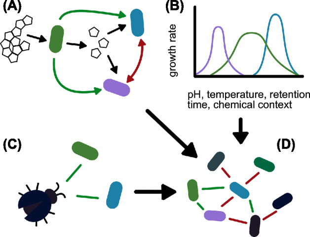
Sources of co-occurrence in microbial interaction networks. (A) Co-occurrence relationships can be driven by microbial interactions. Cross-feeding between species can be detected as co-occurrence relationships, while competition can cause mutual exclusion. (B) Organisms that share niches are more likely to co-occur. If samples were taken from a heterogeneous environment, differing niche specialization may induce spurious interactions. (C) Not all interacting species are detected in a 16S rRNA dataset. (D) The final inferred network contains both spurious and true interactions.

Indirect edges can be a result of sample heterogeneity. Such heterogeneity occurs when environmental factors differ within the studied ecosystem and may be a result of experimental design. The phenomenon is problematic when network analysis is used to infer associations. As a result of diverging niche preferences of microbes, shared niche preferences in a variable environment can be a source of co- occurrence patterns. When two species have growth optima in the same niches, they will co-occur, while the opposite effect will result in mutual exclusion. Niche preference may also explain why closely related species frequently co-occur, as they are likely to have more niche overlap than more distantly related species (Chaffron et al.2010; Faust et al.2012; Pascual-García, Tamames and Bastolla 2014).

Despite the possible influence of niche preferences on network structure, network inference tools often do not incorporate environmental data. This can result in a sharp increase in environmentally induced indirect edges. Tools based on inverse covariance such as SPIEC-EASI are theoretically able to remove these edges, under two assumptions: first, that the data are multivariate normally distributed and second, that all components of the systems have been considered. The first assumption can be relaxed, but the second is not so easy to tackle in the presence of a variable environment.

Regardless, a good sampling strategy can mitigate the effect of niches. Investigators may work with controlled environments, such as bioreactors or artificial biofilms. In such situations, niche preferences are less likely to cause spurious associations, as sample variation is reduced and remaining niches (e.g. anoxic zones in the biofilm) can be accounted for with a thorough monitoring strategy. In less structured environments, investigators can choose to split up a dataset when there are large differences between sets of samples that can be attributed to environmental factors. This could be justified because associations between relevant taxa and environmental factors have previously been described in the literature, or because the environmental features correlate to community variation. Alternatively, the effect of niche preferences can be mitigated by selecting for generalist species. Investigators can choose highly heterogeneous samples and set a stringent prevalence filter; consequently, only species occurring in many samples will be preserved. Pascual-García, Tamames and Bastolla (2014) used this approach to study cosmopolitan species. They were able to find species that co-occurred across different environments, and showed that some of these co-occurrences were supported by the literature and therefore likely represented biotic interactions.

While niches can introduce environmentally induced indirect edges, the visualization of environmental influence is a major strength of association networks. Most researchers collect additional clinical or environmental data in their microbiome studies, which can be included in an integrated network. Visualizing niche preferences can be valuable in systems where little is known about the microbes of interest, and in fact, recent observations on macro-ecological co-occurrence networks have shown that these networks may represent niche preferences better than they represent biotic interactions (Freilich et al.2018). The networks’ sensitivity to environmental factors is also beneficial for the reconstruction of community structure. Network-based measures of β-diversity, such as TINA and PINA, resolved habitat-induced clusters in the human microbiome more clearly than other approaches (Schmidt, Rodrigues and Von Mering 2017)

Moreover, networks can represent niches as mediators of microbial interactions. Some microbes change environmental properties to create new niches. They may cause acidification, provide spatial structure or remove oxygen from the environment (Ziegler et al.2013; Welch et al.2016). Co-occurrence patterns can show microbes' abilities to generate spatial structures or an anaerobic environment. For example, early and late colonizers in dental plaques are negatively associated (Faust et al.2012). This is not a direct interaction, but the result of aerobic bacteria creating an anaerobic environment that favours the oxygen-sensitive late colonizers (Kolenbrander et al.2006; Welch et al.2016).

Of all the discussed network inference tools, few support inclusion of environmental or host data. For example, CoNet computes associations between taxa and environmental factors such as pH or host metadata such as weight. MInt assumes that there is an additive linear influence of environmental or host factors on species abundances. It removes this influence by first regressing out these factors and then inferring the taxon network from the residuals (Biswas et al.2016). Associations between taxa and environmental factors are usually computed for relative abundances. It remains to be evaluated to what extent conclusions based on these associations hold for absolute abundances.

Correlations to environmental abundances are not the only approach to include environmental data. For categorical variables (e.g. sampling method or location), appropriate differential abundance tests such as those implemented in ALDex2 or DESeq2 can be used (Love, Huber and Anders 2014; Fernandes et al. 2013). Species that are differentially abundant could then be connected to a node representing the environmental factor of interest, or the effect size could be added as a node property. If investigators include such data in a network, it may become more obvious how certain modules of the network represent environmental conditions, even though not all species of the modules may be significantly differentially abundant. As networks are a flexible form of data storage and visualization, there is little reason to limit them to abundance data.

BIOLOGICAL INTERPRETATION OF NETWORK PROPERTIES

With microbial associations only predicting biotic interactions in a minority of cases, emergent properties may be more reliable in the search for new biological insights. Microbial interaction networks provide an excellent tool for studying them. Abstract concepts from network theory may hint at biological emergent properties, such as antibiotics tolerance in microbial communities, where microbes lacking resistance genes can tolerate antibiotics if they are part of a community (Kim et al.2013; de Vos et al.2017). However, the link between these concepts and experimental observations is unclear. In this section, we address the following network properties: hub species, betweenness centrality, network motifs, assortativity, transitivity, modularity and network robustness. A graphical summary of these properties is provided in Fig. 2.

Figure 2.

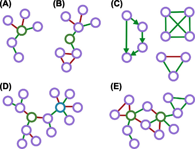
Emergent node properties in networks. (A) Network with the green node representing a hub, as it has the highest degree. (B) Network with the green node having the highest betweenness centrality. (C) Examples of motifs that can be found in networks. The feed-forward motif: (here, a 4-node motif is shown) is a known motif in gene regulatory networks (Shen-Orr et al.2002), while the clique and triad motifs are examples of motifs that can be found in undirected microbial networks (Ma and Ye, 2017). (D) Assortativity in a network. The green node is assortative, because it only connects to other nodes with the same degree. The blue node is disassortative. (E) Fragility or robustness in a network. This network is fragile to targeted attacks, because any attack on the green nodes fragments the network.

Defining node importance in networks

In the search for meaningful biological knowledge, hub species are frequently an outcome of microbial network analysis. Hub species are nodes that have the highest degree in the network and are therefore associated with a high number of other species. Identifying these species is straightforward, and their importance to community structure seems almost intuitive. Yet, the ecological role of hub species is still unclear. For example, hub species may represent keystone species, which are known to be important for ecosystem structure and functioning. Their removal can cause the ecosystem to collapse (Paine 1969). Hub species do not necessarily share the same biological implications, as investigators cannot infer such major changes unless they carry out experiments that involve removal of hub species and randomly selected control species (Berry and Widder 2014). Moreover, recent work has demonstrated that known keystone species in macro-ecological networks do not necessarily result in detectable signals in co-occurrence networks (Freilich et al.2018). This further weakens the assumption that hub species are likely to represent keystones.

A related concept to hub species are the Strongly Interacting Species (SIS) (Gibson et al.2016). In simulations, these ‘levers’ were shown to be able to steer ecosystems towards certain community types. For these community shifts to occur, heterogeneous interaction strengths are necessary, with SIS having the strongest interactions. Overall, the role of hub species in community structure is poorly defined and may contain aspects of keystone species as well as lever species. In general, without further experimental validation, it is unclear whether predicted hub species or SIS act as keystones or levers in the ecosystem of interest.

Beyond degree, other types of node centrality can be a proxy for node importance (Borgatti 2005). For example, the betweenness centrality of a node is calculated as the total number of shortest paths from all nodes to all other nodes that pass through the node (Freeman 1977). Therefore, a node that has a degree of two can have the highest betweenness centrality in a network if it connects clusters that make up the network. Despite its low degree, it can affect large sections of the network. Apart from shortest paths, random walks through a network can also be used to estimate node centrality (Newman 2005). Nodes that are visited more frequently during a random walk are then assigned greater centrality estimates. Other forms of centrality exist as well, each making different assumptions on the nature of interactions between nodes. For example, betweenness centrality assumes that the shortest path matters (e.g. package delivery from one location to another), whereas centrality measure based on random walks assumes that information or metabolites travel randomly (e.g. gossip in a social network). Applying the wrong centrality measure to a network can result in incorrect measures of node importance (Borgatti 2005). As the mechanisms behind microbial interactions may be diverse and are generally unknown, we cannot recommend an optimal choice for centrality measures of microbial networks.

Moreover, some measures of centrality rely on the simulation of movement on networks. Their interpretation and relevance differs depending on the type of network; walks on an undirected network faces fewer limitations than walks on a directed network. Hence, directed networks constructed from time series data represent community structure differently from undirected networks constructed from cross-sectional datasets. Fig. 3 showcases this issue. In the undirected network shown in Fig. 3A, the blue node appears to be a hub species. However, as the directionality pattern in 3B shows, it benefits from the presence of other species, but does not influence them. In the directed network shown in Fig. 3B, the blue node appears to be a ‘dead end’, whereas walks can pass freely from the grey node to other nodes. Hence, simulations that rely on random walks will indicate that the grey node is the most influential one, as most random walks will pass through it.

Figure 3.

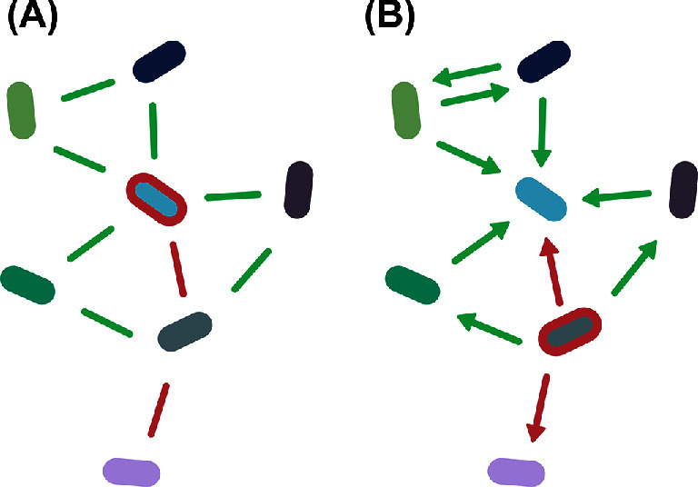
Node directionality can influence node importance. (A) In this undirected network, the red-bordered blue node scores best on centrality measures. As movement across this node is possible, in silico simulations of random walks, shortest paths or other types of movement will support the hypothesis that this node plays a key role in network structure. (B) In this directed network, in silico simulations of movement processes will not traverse the blue node. Hence, the red-bordered grey node can now be identified as having the most influence.

Linking network properties to biology

While measures of centrality describe network components, higher level descriptions of networks may be informative as well. For example, a motif is an overrepresented subnetwork with at least three nodes, with overrepresentation meaning that the motif occurred significantly more often than expected by chance (Milo et al.2002). Motifs have frequently been found in gene regulatory networks, and models have shown that they can stabilize signals in transcriptional networks (Shen-Orr et al.2002). Hence, they may play a role in efficient and robust flows of information in intracellular signalling pathways. Regardless of their function, investigators have used motifs to identify key regulators in gene regulatory networks (Green et al.2018).

Microbial networks differ from gene regulatory networks with respect to selection pressure. While genes and gene motifs are conserved due to unique, vital functions that these genes provide, host-associated microbial communities may contain more redundancy and express more opportunistic behaviour. Yet, they are also exposed to selection on the community level, as microbes’ intimate associations with their hosts imply that they experience at least part of the selection pressure their hosts face. To mitigate opportunistic behaviour by microbes, hosts have evolved several strategies to control community composition (Walter and Ley 2011; Foster et al.2017). This unique selection pressure may lead to patterns in community structure, but it is not evident what those patterns would look like in a microbial network.

At this point, the role of motifs in microbial networks has not been established. It is possible that such motifs represent conserved information transfer or conserved cross-feeding interactions. Information transfer could involve processes such as quorum sensing or electrical communication. Inter-species communication has been observed in aquatic environments and human pathogens (Canovas et al.2016; Mori et al.2017). Similarly, microbes can use electrical communication to coordinate metabolic activity in biofilm communities (Prindle et al.2015). Even if direct interactions have not been demonstrated, microbes may change their transcriptome in response to other species (Plichta et al.2016). The ability to coordinate behaviour on the inter-species level suggests that microbes can collaborate. If conserved, such relationships could form motifs.

Currently, the presence and function of motifs in microbial networks remains confined to speculation. There are already hints that they may at least be useful as biomarkers. Ma and Ye (2017) investigated the presence of triad motifs in human microbiome datasets. They found that specific motifs were over- or underrepresented in multiple diseases. We still do not know if such patterns are conserved across ecosystems (or even across tools) or why they would be there. Establishing the role of motifs in microbial networks requires more exploratory research.

Similar to motifs, assortativity coefficients describe network structure. In an assortative network, nodes are more likely to connect to similar nodes. Multiple definitions of this similarity exist. Firstly, assortativity may be defined as similarity in node degree (Newman 2002). Based on this definition, Newman was able to calculate assortativity scores for multiple networks, with positive assortativity scores indicating that nodes are more likely to connect to nodes with similar degree. In contrast to social networks, Newman (2002) found that biological networks were disassortative. He demonstrated with a model that assortative networks are broken up less easily by removing high-degree nodes than disassortative networks.

Although Newman defined similarity with respect to node degree, similarity can also be calculated with respect to in- or out-degree for directed networks. The majority of microbial network inference tools do not provide directed networks, but assortativity could also be defined as similarity in co-occurrence or mutual exclusion. Investigators may also use local assortativity, where the degree is only compared to the degree of a node's direct neighbours. Piraveenan, Prokopenko and Zomaya (2012) observed that many biological networks are assortative rather than disassortative when these alternative coefficients are used. Hence, assortativity coefficients should be interpreted carefully in the context of microbial networks, as the definition of assortativity employed changes the outcome entirely. Moreover, assortativity may also refer to similarity in taxonomic group (Kurtz et al.2015). This type of assortativity indicates whether species are more likely to interact with closely related species. While such a coefficient contains more biological information, it is less amenable to evaluations based on network theory.

While assortativity refers to heterogeneity of edges in a network, transitivity describes heterogeneity of global structure, i.e. it quantifies the extent to which nodes cluster together. Hence, this property is also referred to as the global clustering coefficient. To the best of our knowledge, transitivity has not been reported to be informative for microbial networks. In social networks, transitivity quantifies the statement ‘Friends of my friends are friends’ (Burk, Steglich and Snijders 2007). While microbes do not have friends, they can display cross-feeding, and high transitivity might be indicative of degradation pathways or niche filtering. However, as we may not be able to estimate assortativity or transitivity without knowing the true interaction network, these coefficients may have little bearing on the interpretation of inferred networks. Currently, we do not know whether they may be consequences of community properties such as evenness (Faust et al.2015b).

Finally, modularity quantifies to what extent networks can be broken up into smaller components. For the identification of such modules, a rich toolkit is available. For instance, the Markov Cluster algorithm simulates random walks through a network to define clusters (Dongen 2000; Van Dongen and Abreu-Goodger 2012). While the Walktrap algorithm also relies on random walks, it benefits from lower runtimes and can therefore handle larger networks than the Markov Cluster algorithm (Pons and Latapy 2005). An algorithm developed by Newman and Girvan (2004) separates networks into modules by iteratively removing the highest betweenness nodes in the network. As each of these algorithms returns modules with different structural properties (i.e. highly compact modules or a minimal number of inter-module edges), their performance in module identification differs depending on the desired properties of a module (Leskovec, Lang and Mahoney 2010).

Regardless of the choice of algorithm, the source of modularity in microbial networks is not entirely clear. Modules may visualize different niches and have been used to study habitat preferences, for example, in soil (Chaffron et al.2010). In another example, Guidi et al. (2016) studied carbon export in plankton communities sampled during the TARA Oceans expedition and found that two modules were associated with this process. One module contained prokaryotes and explained approximately 60% of the variation in carbon export. The other module contained phages and could predict 89% of the same variation. Interestingly, the most important nodes in these networks were Synechococcus, a cyanobacterium and two Synechococcus phages. This indicates how these modules represented carbon export as an interplay between phages and their hosts and shows the potential of network modules as indicators of important ecological processes.

Although the study system may be the same, drivers behind the modules can differ. In another study on free-living communities in a marine ecosystem, modules were shown to correspond to the depths where samples were collected, supporting the existence of environmentally driven modules (Cram et al.2015). Cram et al. identified two modules, one of which corresponded to surface chlorophyll and daylight length. It may be challenging to distinguish modules due to shared pathways and cross-feeding from those introduced through environmental factors. For example, Jiang et al. (2015) observed that modules corresponded to soil variables as well as potential nitrification activity. The difference between these may be impossible to identify when little is known about the organisms in a module.

Overall, modules may be indicative of ecological processes governing community structure, but further information is required to identify their origin. In part, this information can be gathered from overrepresentation of specific functions or taxonomic groups in a module. If specific groups of enzyme-coding genes are overrepresented, the taxa in the module may be specialized on a specific nutrient. The metabolic pathways concerned may be inferred from the overrepresented genes. For example, a network of forest soils could contain a module with species that play a role in nitrogen fixation (Menezes et al.2015). Alternatively, if taxa are overrepresented, this could indicate the effect of niche filtering.

Network robustness is an in silico property

Newman (2002) posed that assortativity can be an indicator of network robustness. However, how is robustness measured in the context of microbial networks? First, we would like to clarify that we are not referring to robustness in the statistical sense, where robustness means that method choice does not affect research outcomes (Huber 2011). While this definition of robustness has value to microbial networks and would ideally be reported, the next section focuses on robustness as a concept from network theory.

Robustness, as a network property, can be studied using percolation theory (Cohen et al.2000). This theory describes how information can flow from one node to the next. One of its applications is to model the effect of node removal on a network. In this context, robustness refers to a network's vulnerability to random or targeted node removal, where the network is considered vulnerable when it breaks up in smaller parts as a result of node removal. The percolation threshold is a quantitative measure of network vulnerability: when enough nodes are removed to move past this threshold, the network breaks down and the size of its largest component decreases sharply (Cohen et al.2000).

The robustness of biological networks is closely related to their degree distribution. This distribution of biological networks does not always follow a power law (where the degree distribution of the network have a heavy-tailed distribution), but there are frequently many more nodes with low than high degree (Camacho, Guimerà and Amaral 2002; Khanin and Wit 2006; Lima-Mendez and van Helden 2009). As only few nodes have high degree and are therefore hubs, biological networks are in theory robust to random node removal, but sensitive to targeted node removal (Albert, Jeong and Barabási 2000; Kwon and Cho 2008). While percolation is difficult to demonstrate in practice, it is possible to compute which nodes are influencers. Influencers may be an in silico alternative to keystones, as removal of influencers causes a network to fragment (Morone and Makse 2015).

There is also a third definition of robustness in the ecological sense, which is defined as the capacity of an ecosystem to maintain its current state despite fluctuations in the behaviour of its member species or its environment (Mumby et al.2014). For example, the taxonomic composition of the gut microbiome may not be robust to dietary changes (David et al.2014), even when the functional composition does display robustness (Eng and Borenstein 2018).

To the best of our knowledge, there are no extensive evaluations on the use of percolation theory in microbiome research. Node removal analysis may not predict how systems respond in real life, since the network is only a simplified representation of the ecosystem. Moreover, while all association networks are static representations of ecosystems, directed networks inferred from time series may be more suitable for node removal simulations. Regardless, network robustness is far easier to evaluate than ecological robustness, and would therefore be a valuable diagnostic tool if it is predictive of ecological robustness.

FROM A NETWORK TO A HYPOTHESIS

In the previous section, we addressed the nature of edges. We also hinted at how to improve experimental design to uncover or avoid sample heterogeneity. Inclusion of additional information may allow researchers to distinguish indirect from direct edges and to elucidate functional mechanisms behind co-occurrence. Here, we provide examples of this approach.

Environmental information can be included in networks

Lima-Mendez et al. (2015) studied the Tara Oceans plankton dataset, which is unique in the area and range of organism sizes covered: samples were taken at two depths in eight oceanic provinces and included organisms ranging in size from viruses to small metazoans. As addressed previously, studying the effects of biotic and abiotic factors on ecosystem structure poses a problem for network construction: environments with changing abiotic factors can cause spurious co-occurrences to appear. The authors attempted to tackle this problem by including all measured abiotic factors. Their initial network contained both environmental factors and taxa, which often formed triplets where two taxa were positively or negatively associated with the same environmental factor. Such triplets suggest that the edge between the two taxa is a consequence of their response to the environmental factor. To quantify the extent of indirectness in a triplet, they calculated its interaction information. Taxon edges in triplets with significantly negative interaction information were assumed to be due to an environmental factor and removed. 42% of previously known plankton interactions were found in the network, and a previously unknown, strongly significant candidate interaction was validated with confocal laser microscopy.

In a similar manner, Wang et al. (2016) investigated lung microbiome data collected from patients with chronic obstructive pulmonary disease. Previous studies indicated that an increase in disease severity was associated with a decrease in α diversity (Rogers et al.2004; Zakharkina et al.2013; Huang et al.2014). Wang et al. (2016) exploited host metadata to find taxa that would play a role in this dysbiotic state. After excluding collinear variables, 66 clinical variables were included in the integrated network. Consequently, they found that several sputum biomarkers were hub nodes in the co-occurrence network. These biomarkers were mostly associated with inflammation, indicating that the dysbiotic state was correlated with an inflammatory response in the patients. They suggest that specific hub species were drivers of the inflammatory response.

Identifying key players in the microbiome

While Agler et al. (2016) did not include metadata in this way, they carried out in silico experiments to quantify the importance of hub species in the Arabidopsis microbiome. The Arabidopsis phyllosphere (above-ground plant surface) network contained three hubs that were correlated to most other nodes. Agler et al. (2016) hypothesized that those nodes had a disproportionate effect on the ecosystem. To test this hypothesis, they performed a node removal experiment in silico, where they removed each of the hubs and observed that their removal affected more edges than removal of non-hub species did. They then confirmed the effects of two hubs, Albugo sp. and Dioszegia sp., through host colonization experiments and interaction assays. As Albugo needs a living host to survive, they were unable to study individual interactions. Nonetheless, host colonization experiments showed a decrease in microbial α diversity on infected Arabidopsis plants. For Dioszegia, interaction assays revealed that this hub reduced leaf colonization efficiency of some bacteria. Their approach demonstrates how causal relationships can be tested with species that cannot ordinarily be cultured and how keystone behaviour of identified hub species can be experimentally validated.

Microbial networks may be especially valuable in the study of pathobionts. Unlike true pathogens, pathobionts can be present in the microbiome of healthy individuals. As a result, identifying causal relationships between a pathobiont and a disease is not as straight-forward, but network analysis can help elucidate the principles through which pathobionts cause disease. Meyer et al. (2016) approached Black Band Disease in coral metaorganisms in this manner. As Black Band Disease is a polymicrobial infection, there is no single causal agent. However, one cyanobacterium, Roseofilum reptotaenium, was present in most samples taken from black bands (Miller and Richardson 2010). Meyer et al. (2016) first compared healthy to diseased coral microbiomes. They found that the microbiomes of healthy corals were more uniform than those of diseased corals, further supporting the validity of the Anna Karenina principle (Zaneveld, McMinds and Thurber 2017).

As R. reptotaenium is present in healthy coral as well, the authors hypothesized that it was not a primary pathogen and interactions in the microbiome were responsible for disease progression. Indeed, they found that genera associated with diseased microbiomes co-occurred with other disease-associated genera. The position of R. reptotaenium in the network was particularly interesting, as its low number of associations linked it mostly to highly connected species. The authors’ follow-up analysis on R. reptotaenium showed that it was indeed directly affecting highly connected hub species through a compound that disturbed quorum sensing, thereby altering microbial interactions. Overall, the network structure successfully highlighted the pathobiont's mechanism of infection in addition to its importance in disease progression.

Network approaches have also been applied to mouse studies. In such studies, causal relationships are more readily observed than in clinical trials. Standardization of mouse studies implies reduced sample heterogeneity, and as these studies are better controlled, it is more likely that changes in network structure are the result of microbial interactions rather than environmental factors. For example, Mahana et al. (2016) investigated the effect of antibiotics treatments on mice fed with a high-fat diet. Mice treated with antibiotics had increased adiposity compared to untreated mice on the same high-fat diet. They applied unsupervised clustering on physiological data to cluster samples in six groups. Most of the clusters corresponded to specific phenotypes (e.g. mice on antibiotics or young control mice). The authors then constructed separate networks for each cluster. To compare them, they identified potential keystone species. They quantified network robustness by performing targeted node removal and suggest based on this analysis that specific antibiotics could target keystone taxa and result in ecosystem collapse. While this is an attractive hypothesis, their analysis was conducted in silico, and the ecological role of hub or bottleneck taxa is still not fully understood.

The above approaches highlight two key strategies to learn more from microbial networks. Firstly, networks can integrate measurements of environmental parameters. We cannot recommend a standard parameter set; each of the studies above included their own relevant parameters. A good understanding of the ecosystem under consideration is therefore vital for experimental design. In many studies, abiotic parameters or biomarkers will be measured regardless of their use in network construction. However, while the data are there, incorporating it is not yet a trivial exercise, since no microbial network inference tool supports all types of environmental data. Categorical data may also guide the division of data into groups, for instance according to treatment. A separate network can then be constructed for each group, as Mahana et al. (2016) did. This can reduce sample heterogeneity.

Secondly, researchers can apply concepts from network theory and percolation theory to further analyse their networks, as demonstrated by Agler et al. (2016) and Mahana et al. (2016). As promising as their work is, it is unclear how predictive in silico results are of ecosystem behaviour, and experimental verification remains a necessity.

Properties of inferred networks are not reliable

Overall, most of the properties we addressed above can be calculated in a straightforward and user-friendly manner. Yet, the effect of environmental conditions and tool choice on emergent properties is unclear, and it is therefore unknown if emergent properties can be inferred reliably from microbial networks. Following Berry and Widder (2014), we generated interaction matrices with the Klemm–Eguíluz algorithm and simulated community dynamics with the gLV equation. Not all microbial communities may follow gLV dynamics. For instance, their dynamics may be better described by neutral models (Sloan et al.2006), and gLV-type models may be unable to correctly describe all interaction mechanisms (Momeni, Xie and Shou 2017). Nonetheless, despite their simplifying assumptions, studies have demonstrated the merit of gLV models in microbiome analysis (Bucci and Xavier 2014; de Vos et al.2017). The simplicity of these models makes them easy to implement and fast to solve numerically in simulations.

As there are no fully verified microbial interaction networks, we can only estimate their topology. However, Sung et al. (2017) showed that only 17.6% of gut microbes in a literature-curated gut microbial interaction network were highly connected. Experimental work has also shown that inferred networks could be fitted to a (truncated) power law (Zhou et al.2011). Moreover, food webs have been found to have skewed degree distributions (Solé and Montoya 2001; Dunne, Williams and Martinez 2002). Overall, this supports the existence of hub species in microbial networks, and those can be simulated with the Klemm–Eguíluz algorithm, which generates networks through preferential attachment (Klemm and Eguíluz 2002). Consequently, we generated synthetic interaction networks with this algorithm and then used these ‘known’ networks to test tools’ abilities to infer emergent properties from data. A graphical summary of the simulation is provided in Fig. S1 (Supporting Information), while a more elaborate explanation of the methodology and a code repository are provided as supplementary files.

Network structure is changed by sample heterogeneity

To study the effect of environmental factors, we changed growth rates in half of the samples in each dataset, effectively simulating different environmental conditions in a single dataset. A similar approach included environmental parameters in a gLV model before, and this model could be fitted to seasonal fluctuations in a lake population (Dam et al.2016).

We expected the increasing environmental influence to be accompanied by a decrease in precision, as more environmentally induced indirect edges are formed. This is indeed reflected in Fig. 4B and 4C. While not all tools reported an increase in degree (especially SPIEC-EASI kept inferring sparse networks), precision decreased for all tools. Moreover, the environmental factors changed the network structure, as transitivity increased markedly. While the transitivity is expected to increase as the degree increases, it also increases for tools that do not report a sharp increase in degree. The differences between the SPIEC-EASI algorithms is especially noteworthy, as the changes in precision are not drastically different between the two, whereas the transitivity coefficients are. Moreover, the small increase in degree indicates that the networks inferred by SPIEC-EASI are rewired as the environmental factors become stronger.

Figure 4.

Network statistics for association networks inferred by CoNet, gCoda, SparCC, Spearman correlation and SPIEC-EASI from datasets with increasing environmental strength. For CoNet, two p-value merging methods were tested: Fisher p-value merging and Brown p-value merging. For SPIEC-EASI, two different algorithms were included: the graphical lasso as well as the Meinshausen–Bühlmann method. These settings are referred to as GL and MB. (A) Scatterplot of precision versus sensitivity for all generated networks. Sensitivity measures how many of the known interactions are predicted, whereas precision quantifies how many of the predicted interactions are correct. In (B-E) a quadratic function was fitted to the data points, and the gray area represents the 95% confidence interval for the predicted quadratic function. (B) Average degree for all networks, with the average degree for the Klemm–Eguíluz matrices indicated at x = 0. The average degree increases drastically for CoNet and Spearman. (C-E) Precision, assortativity and transitivity of all networks. Precision decreases for all tools when environmental strength increases, whereas transitivity increases. However, no general trend can be observed for assortativity.

Finally, Fig. 4D indicates how assortativity varied wildly for all tools across conditions. Assortativity is generally assumed to be negative in biological networks. The Klemm–Eguíluz interaction matrices reflect this. Yet, most tools fail to return a negative assortativity; if they do, that changes once the dataset conditions change. For SPIEC-EASI, positive assortativity can at least partially be explained by the low number of edges (sparsity) of its inferred networks. With nodes in the SPIEC-EASI networks following a narrower degree distribution, they are less likely to be disassortative as there are fewer high-degree nodes to connect to. In contrast, networks inferred with CoNet have negative assortativity scores at low environmental strength, but the scores become positive when the influence of the environment increases. This may be explained by an increase in node degree once CoNet starts correlating species as a result of environmental factors.

Global network properties in inferred networks frequently failed to match the values measured in the Klemm–Eguíluz interaction matrices. Network theory provides a valuable resource, but some measures may not be suitable for microbiome studies. As topological characteristics of networks are easily calculated with the R igraph package or within Cytoscape, authors do sometimes report them in a publication. Based on our simulation, it seems unwise to attribute biological relevance to such properties in the absence of experiments or additional information. If the underlying interaction network is unknown, they are as likely to be a result of tool bias as they are to be a result of organized, complex behavior. These results reflect those obtained by Connor, Barberán and Clauset (2017), who showed that network properties can change entirely when threshold settings for Spearman correlation are altered.

As we mentioned previously, modules may represent different niches. Hence, we would expect the introduction of two niches in our dataset to generate a modular structure of the network. Fig. 5 displays this structure for datasets from one specific Klemm–Eguíluz matrix.

Figure 5.

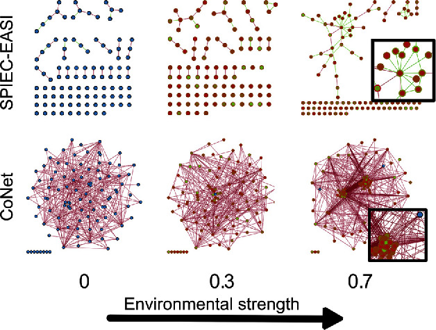
Network structure across the environmental gradient for networks inferred with SPIEC-EASI and CoNet. SPIEC-EASI was run with the Meinshausen–Bühlmann method, while CoNet used Brown p-value merging. For visualization of SPIEC-EASI networks, a circular layout was used, while the CoNet networks were visualized with a force-directed layout that takes edge sign into account. Two modules become visible as the environment becomes stronger. Similar to the modules found by SPIEC-EASI, those displayed in the CoNet 0.7 network are connected by positive edges. The fill and border colours of the nodes indicate the effect of the two environmental conditions on growth rates, with green implying that the condition has a positive effect on the growth rate and red implying a reduced growth rate. In the last two CoNet networks, the blue nodes represent environmental factors.

Notably, two clusters are formed when the environmental strength is increased. The colours of the nodes indicate that this is indeed a result of similar responses to the environment. While SPIEC-EASI still generated a sparse network, additional positive edges were formed between similarly-colored nodes, and a few negative edges appear between dissimilar nodes. In contrast, the degree increased drastically with environmental strength in CoNet. This structure was only visible for the simulated datasets where there are distinct groups of microbes that respond differently to a strong environmental factor, so the effects of the factors are completely reversed for each of the groups in half of the dataset. We did not enforce this constraint, so not all of the inferred networks share this structure.

This modular structure could not be identified without edge signs, as the modules consisted of co-occurring (as opposed to mutually exclusive) species. Our synthetic environment therefore appears to mimic the effects observed in experimental studies (Chaffron et al.2010; Cram et al.2015; Jiang et al.2015). Moreover, experimental results suggest that modules may be consistent across tools even when specific edges are not (Wang et al.2017). However, clustering approaches to identify such modules need to take the edge sign of microbial associations into account.

Centrality is different for each tool

As degree and betweenness centrality are of interest to microbial ecologists, we evaluated whether tools could identify species with high degree or a high betweenness centrality score.

For the highest degree species, abundance is generally very low. Since the interaction matrix used in the gLV simulations has a low percentage of positive edges, highly connected species have a higher chance than low-degree species to be exposed to negative interactions. As only SPIEC-EASI and CoNet attribute high degree to low-abundance species, this may explain their better performance in this simulation (Fig. S3, Supporting Information).

Fig. S2 (Supporting Information) shows that tools scoring high on precision are not necessarily the ones performing best when searching for hub species or highest betweenness centrality species. Even changing the settings for one of the SPIEC-EASI analyses caused a marked change in identified hubs. Moreover, while gCoda and SPIEC-EASI both scored well on precision, they did not score equally well when identifying hub species. The simulation shows that precision is not the only measure that should be incorporated when testing tools for emergent properties, although it is vital for interaction prediction.

There is a striking lack of overlap in identified hub species, as tools mostly identify unique hubs (Fig. S4, Supporting Information). This matches an experimental study on a paddy soil microbiome, where most hub species were not conserved across tools (Wang et al.2017). As the tool predictions rarely overlap and the overlap was not enriched in true positives compared to individual tool predictions, we doubt whether an ensemble approach incorporating multiple tools will increase the accuracy of hub species inference.

Accuracy increases when the top percentage is evaluated

Previous work indicates that the sensitivity of degree and betweenness centralities to errors decreases when more nodes are considered, rather than the top 1 or top 3 hub nodes (Borgatti, Carley and Krackhardt 2006). We wanted to confirm this for our analysis and calculated the number of correctly predicted hubs when we analysed the top 3, 5, 7, 10, 20 and 30 hub species. In this case, we investigated the overlap between hub nodes in the true positive network and in the inferred networks, which is one of the most stringent measures of accuracy assessed by Borgatti and colleagues. A less stringent approach would be to test whether the highest centrality node is present in the top 10%.

Fig. 6 shows how the number of correct predictions increases as more nodes are evaluated. For example, if the top 10 hubs are taken from a network inferred with CoNet, approximately half will be correct; if the top 20 are taken, this increases to 11 correct predictions on average. Moreover, we computed p-values using the hypergeometric test, which gives the probability of drawing the observed number of correct hubs by chance. The p-values stop decreasing after more than 20 hub species are identified. This is likely to be an innate property of our true positive network, as exceeding this 20% means the degree of species is no longer part of the tail of the degree distribution, i.e. these species are no longer hubs.

Figure 6.

Number of correct predictions and p-values in networks inferred with CoNet, gCoda, SparCC, Spearman correlation and SPIEC-EASI. In both figures, the standard deviation is shown. For CoNet, two p-value merging methods were tested: Fisher p-value merging and Brown p-value merging. For SPIEC-EASI, two different algorithms were included: the graphical lasso as well as the Meinshausen–Bühlmann method. These settings are referred to as GL and MB. (A) Mean number of correctly predicted hubs for increasingly large sets of hubs. A quadratic equation was fitted to the data points. (B) Mean p-values for increasingly large sets of hubs, with the p-values calculated individually for each replicate. These values were calculated from the hypergeometric test, where the p-value represents the probability that the correctly predicted hubs were drawn randomly from the population (n = 100). Values below the purple line are smaller than 0.05.

However, as none of the tested tools identified hub species well, identification and interpretation of hub species should be handled with care in real datasets. This implies that inference of hub species may be more accurate when ∼10% of high-degree hubs are studied rather than a select few. Moreover, the gLV simulation produced high-degree, low-abundance species, and not all tools appeared to be able to identify these. While analyses on the human microbiome and farm soils have also identified highly connected, low-abundance taxa (Faust et al.2012; van der Heijden and Hartmann 2016; Claussen et al.2017), we do not know whether the associations between those are true biotic interactions.

NETWORK INTERPRETATION BENEFITS FROM DATA INTEGRATION

Even in our relatively simple simulation, networks were often dense and difficult to interpret. The situation is worse in practice: most investigators will find a ‘hairball’ network when they start analysing their datasets. Reducing the size of that hairball down to a more informative version of itself is necessary before follow-up experiments can be done. For studying individual interactions, a low number of false positives is a requirement. It would also be useful to have more information on the interactions themselves. Once an investigator knows which associations are statistically robust and what mechanisms they represent, follow-up experiments can be reductionist without needing to be excessively high-throughput. For that purpose, we discuss some methods to reduce the number of edges in a network and to identify the mechanisms behind them.

Agglomeration and prevalence reduce node number

Agglomeration and prevalence filtering are relatively simple to perform, as they require no additional data nor well-annotated species. Agglomeration can ‘set’ network detail at the taxonomic level. Researchers can apply an agglomeration step before network inference to study microbial networks at higher taxonomic levels. If species share specific functions with their phylogenetic group, their abundance may vary randomly, even though the total abundance of the higher phylogenetic group can be stable as a result of the unique function. An agglomeration step will filter out noise induced by these phylogenetic similarities, while revealing conserved interactions at higher taxonomic levels. As an example, Yun and Cho (2016) visualized how specific orders correlated to environmental factors and showed how different communities were associated with certain metabolites. If researchers are interested in highly conserved cross-feeding interactions (e.g. methanogens and hydrogen-producing bacteria), agglomeration can be beneficial.

In addition to taxonomy, ecological groups may also be used. For plankton, functional types such as autotrophs and silicifiers have previously been defined (Quere et al.2005). Lima-Mendez et al. (2015) grouped species in their network according to these plankton functional types. The agglomerated network suggests that parasites are important interaction partners of many other plankton functional types, whereas silicifiers had less predicted interactions with parasites and grazers than did other functional types.

However, agglomeration steps may result in loss of vital information, especially when strains possess unique functions. For example, the coral pathogen R. reptotaenium was unique in its ability to disrupt quorum sensing networks (Meyer et al.2016). If the network is created at a higher taxonomic level, unique interactions may be ‘diluted’ as relatives do not share the interaction. Unless the reaction is strong enough, it will not be part of the final network. This can be prevented if the agglomeration step is carried out on the constructed network, rather than on the supplied data. In that case, the agglomeration step can retain edges at lower taxonomic levels as part of the metadata, and taxa that have conflicting edge signs despite phylogenetic similarity can be retained as separate nodes.

As mentioned previously, researchers can also choose to filter for high prevalence. This approach is beneficial in reducing sample heterogeneity and in increasing precision of network inference. The only remaining taxa will be more generalist in nature, and interactions for those may be more reliable. Of course, rare taxa will be lost in the analysis. This may be detrimental in some cases, as rare taxa may be more likely to perform unique functions (Jousset et al.2017). Although the goal of species reduction would also be achieved by an abundance filter, a prevalence filter may have less impact on inferred network structure. The influential species simulated by Gibson et al. (2016) were not always highly abundant and would be removed by abundance filters. Moreover, abundance filters do not remove sampling heterogeneity, as highly abundant taxa that are only present in a few samples would be retained.

Visualizing functions in addition to taxa

When species are sufficiently annotated or metagenomics data are available, more detailed information about the community members can be included in the network. While this will not directly reduce ‘hairball’ size, association networks with such information are easier to interpret. For example, KEGG Orthology (KO) profiles or SEED subsystems can be used to predict specific traits or metabolic functions (Overbeek et al.2013; Kanehisa et al.2016). Moreover, metabolic information can reveal functional redundancy when incorporated as a node property.

Integration of functional profiles in networks could also reveal specific niches. In a study on wheat and cucumber, KO profiles were used to identify functional differences between rhizobiomes and soil microbiomes (Ofek-Lalzar et al.2014). The authors found that KOs associated with plant cell wall degradation, motility and chemotaxis were enriched in rhizobial communities, and that some enrichments were specific to the host species. In fact, specialized tools have been developed to perform such comparisons: FishTaco estimates shifts in functional profiles and was used to evaluate differences between healthy controls and a Type 2 diabetes cohort (Manor and Borenstein 2017). In these contexts, the investigators compared KO profiles of different communities. Similar approaches could be used to compare KO profiles of network modules.

While KO profiles have been used extensively, more abstract descriptions of phenotypes may be easier to integrate in a network. For example, the Integrated Microbial Genomes database provides phenotypic annotations, and a standard ontology for microbial phenotypes has been developed (Markowitz et al.2011; Chibucos et al.2014). However, annotating microbial data with these phenotypes is not straightforward, as experimental verification of phenotypes may not be feasible for many species. Moreover, genotype-phenotype matching is not fully reliable (Power, Parkhill and de Oliveira 2017). Hence, ontologies have not been adopted in microbiology as they have been in protein research and genomics. For instance, BugBase provides sequence-based annotation of 16S and metagenomics datasets (Ward et al.2017), but only a limited subset of the phenotypes described in the ontology of microbial phenotypes is currently available. In contrast, FAPROTAX uses functions described in the literature to annotate microbial data (Louca, Parfrey and Doebeli 2016). While it currently describes over 80 functions, its use in understudied microbiomes is limited.

Despite these difficulties, annotation with a suitable ontology, whether this is a phenotype or gene-based one, would allow researchers to better integrate their data in databases and perform interdisciplinary studies (Bard and Rhee 2004). As sizes of databases increase, and interoperability becomes more important, adoption of standard ontologies will be vital to avoid further fragmentation of publically available data. Moreover, ontologies can identify the most informative features in a biological dataset and are therefore useful in data exploration (Mazandu, Chimusa and Mulder 2017). Ontologies also support automated reasoning and could therefore quantify differences at multiple levels of the ontological hierarchy (Rodríguez-García and Hoehndorf 2018). Automated reasoning could be used to report all properties that are unique for each node, module or network, or to suggest phenotypes of uncultured species. For example, an uncultured species assigned to the order Methanomicrobiales could be assigned the methanogen phenotype because all cultured species in that order have methanogen activity. As network analysis is not always carried out by experts on a particular ecosystem, ontologies can support researchers who possess little in-depth knowledge of the ecosystem under scrutiny.

In addition to ontologies, metabolic information can be used to describe specific functions. In the context of networks, metabolic information can be mapped onto edges as well as nodes. As metabolic functions of microbes can differ or overlap, they can indicate metabolic complementarity or redundancy and thus whether edges are likely to represent mutualism or competition. Tools based on metabolic models can provide such predictions. For example, RevEcoR computes metabolite consumption and secretion to provide indices of complementarity or competition (Cao et al.2016). In contrast, MMinte uses flux balance analysis to compute growth rates of species in mono- and co-culture. Tools such as these allow investigators to predict ecological interactions between species. However, metabolic models require the full genome sequence, are limited by poor annotation and may be inaccurate without manual curation (Henry et al.2010). Hence, their use is limited to a small number of well-studied species.

Strikingly, competition for nutrients may result in associations between species, as habitat filtering can have a larger effect on species abundance than competition (Freilich et al.2009; Levy and Borenstein 2013). Hence, predicted competition may appear as co-occurrence in a network, while mutualistic cross-feeding relationships can also be inferred as co-occurrence. Consequently, metabolic information has the potential to reveal more about the nature of associations than co-occurrence alone. Positive associations combined with competition predicted from metabolic models could be indicative of strong habitat filtering.

As far as we are aware, there is no optimal choice for agglomeration steps or metadata choices. Those depend on the quality of the data and the nature of the experiment.

QUANTIFYING THE PERFORMANCE OF NETWORK TOOLS

Due to lacking benchmark data, researchers frequently have to resort to synthetic datasets to identify tool properties. Weiss et al. (2016) evaluate several tools with a synthetic dataset, as we did. Their evaluation shows how tools are affected by some of the challenging aspects of microbiome data, such as compositionality, sparsity and noise. In contrast, we focused on emergent properties and the often overlooked influence of the environment. Our datasets had relatively even species abundance distributions and included no additional noise. Hence, tool performance in our simulation does not necessarily reflect tool performance on actual datasets. However, the simulation highlights to what extent microbial network inference tools differ, both in their response to simulated environmental factors and in their ability to identify hub species.

While both evaluations rely on synthetic datasets, validation through experiments and literature are likely to be even more informative, as these reflect the real-world application of microbial networks. Moreover, analyses that describe the statistical robustness of microbial networks could also highlight problematic conclusions.

Synthetic communities validate networks

Synthetic communities or reduced-complexity communities provide an attractive approach for the validation of microbial networks. As the work from Agler et al. (2016) demonstrates, not all species, such as those that require live hosts, can be cultured for in vitro interaction assays. To remedy this issue, synthetic communities can be established inside or on a host. In contrast to the full ecosystem, these communities reduce the size of the microbiome to a level that is more amenable to dynamic modelling. For example, Arabidopsis has been used to study the effect of reduced-complexity soil communities on plants traits (Panke-Buisse, Lee and Kao-Kniffin 2017). For gut microbes, gnotobiotic mice allow researchers to construct synthetic communities and collect tissue samples, so that the mechanisms behind host-microbe interactions can be studied more easily (Faith et al.2010; Desai et al.2016). For communities that can be cultured in vitro, high-throughput systems are available that support identification of metabolite-driven interactions (Chodkowski and Shade 2017). Hence, synthetic communities serve to validate microbial association networks and in some cases to elucidate the interaction mechanisms behind these associations. However, the extent to which microbial interactions depend on context is not entirely clear, and this may affect the ability of synthetic communities to validate associations from real-world ecosystems. Microbial interactions can vary due to the composition of the background community, and leaving out species or their host to construct a synthetic community changes the context (de Muinck et al.2013; Plichta et al.2016).

In addition to validation of networks, synthetic communities can be used to study dynamics of microbial communities (Vorholt et al.2017). For example, competition may be required for a stable microbiome (Coyte, Schluter and Foster 2015), and synthetic communities could test this hypothesis. Investigators could also perturb synthetic communities and observe the consequences for network structure, as was done for gene regulatory networks (Luscombe et al.2004).

Linking network properties to dynamic behaviour of microbial communities would allow us to discover novel applications of networks as a diagnostic tool. For example, in silico robustness may be predictive of an ecosystem's robustness and may be a tool for management of such ecosystems. Identifying influencers or hub species would allow clinicians to prescribe alternative antibiotics that achieve a shift towards a healthier community state without affecting the entire gut microbiota, as proposed by Mahana et al. (2016). Such applications are still science fiction until a link between these in silico models and experimental observations has been thoroughly established. Synthetic communities may help in the establishment of this link.

In fact, the role of microbial interactions in disease has already been characterized with relatively simple communities. For example, polymicrobial urinary tract infections (UTIs) are caused by bacterial communities. De Vos et al. (2017) constructed an interaction network from mono- and cocultures, which revealed that microbial interactions had two major effects: they resulted in the assembly of highly stable UTI communities, and they provided tolerance to antibiotics for sensitive strains. A study on Drosophila gut microbes showed that higher order interactions were important in the maintenance of biodiversity, and that this diversity affected Drosophila fitness (Gould et al.2017).

Even though validation of microbial association networks may still be out of reach in some (if not most) cases, establishing the effect of context dependency, the biological implications of hub species as well as a better understanding of microbial dynamics already represent valuable contributions.

Benchmark datasets are necessary to develop better tools

Throughout this review, we have demonstrated that network analysis requires investigators to develop unique approaches that answer their research questions. As a result, no standard for data processing or parameter selection is available. Nor is there a ‘one size fits all’ tool. Hence, developing standard protocols for network construction, as was done for amplicon sequencing in the Earth Microbiome Project, is currently not feasible (Thompson et al.2017). This is in part due to our lack of knowledge on tool performance; we have no benchmark dataset to measure tool accuracy. It is also due to the possibility to integrate multiple data sources. The more metadata is included in a network, the larger the effect of multiple testing. Hence, expert knowledge will remain valuable in the selection of relevant biotic and abiotic factors.

However, microbial network inference tools would benefit from standardized benchmark datasets, similar to those developed for microbiome studies or inference of gene regulatory networks (Marbach et al.2010; Sinha et al.2015). What would these benchmark datasets look like? Firstly, there would be no single ideal dataset, but rather, a suite of datasets. While the tools make different assumptions and implement different methods, we do not know the best tool for the job. This is for two reasons; firstly, we do not know sufficiently well which jobs a tool does well (e.g. high-precision prediction of associations, hub taxon identification, module detection etc.), and secondly, we do not yet know which aspects of microbial networks are meaningful for the analysis of real-world datasets. For example, high precision may not be a requirement for accurate assessments of node importance, but we do not yet understand which measure of node importance best reflects the ecological importance of a species.

To tackle that first reason, it is necessary to evaluate biases and limitations that particular tools may have. For example, we found that CoNet and SPIEC-EASI were able to find hub species with low relative abundances, while the other tools did not identify them. Hence, if identification of these species is important, SparCC and gCoda may not be the best choice. At the same time, SparCC may do better when handling datasets with low numbers of effective species (Weiss et al.2016). Revealing such biases requires (simulated) datasets with a pre-specified evenness, species centrality or other property of interest. However, the novelty of such evaluations, especially when repeated on newer tools, may be insufficient to garner interest in the scientific community. Therefore, any such benchmark datasets should be accessible and simple to use to support systematic adoption by tool developers. NeSSM provides an example of such a resource for microbiome sequencing, as it constructs artificial metagenomes from a reference database (Jia et al.2013). With data simulators such as NeSSM, users are able to evaluate how their tools perform on low- versus high-complexity communities, or how they are affected by different sequencing technologies. As it is still poorly understood how data quality and pre-processing affects microbial network inference, network inference tool developers would benefit from such a resource.

However, NeSSM output, as other simulations, may not reflect real-world microbial communities. For example, we assumed in our simulation that microbial communities follow relatively simple Lotka–Volterra dynamics. As real-world communities may only partially be governed by such dynamics and since we did not simulate measurement noise, tool performance on our simulated datasets will differ from the real-world situation. At the same time, in most cases we do not know the interactions and dynamics underlying real-world microbiomes, so performance cannot be evaluated on these datasets. Data from synthetic communities would provide an intermediate representation of complexity. For sequencing analysis, the mockrobiota resource, which contains data from mock communities, serves this purpose (Bokulich et al.2016).

Yet, synthetic communities face similar limitations as mockrobiota: they are still poor reflections of real-world data, as they only contain a fraction of the diversity and noise. While there is no complete ground truth available for real-world datasets (e.g. all interactions and processes have been quantified), a database could be constructed that would contain known associations. This could be used to conclude whether inferred networks are supported by literature, or to more systematically evaluate to what extent network structure reflects ecology. Fig. 7 provides an illustration of such benchmarks. With different types of benchmarks available, we can expect a more diverse range of performance estimators. These would allow users to make more informed choices regarding the network inference tool and the experimental design.

Figure 7.

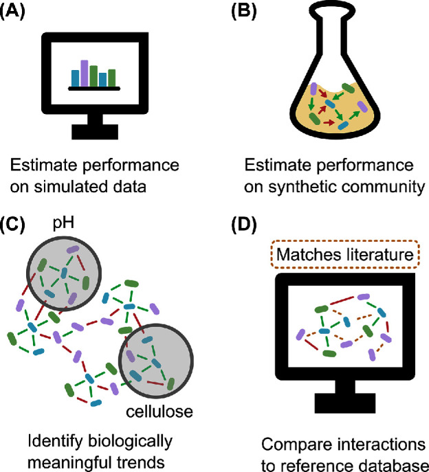
Types of benchmark suites for evaluation of network inference tools. (A) Simulated datasets using different models can help evaluate whether tools are able to identify ecological interactions and network properties. (B) Synthetic communities can provide a ground-truth network with known interactions, which can then be used to evaluate tool precision on real-world data. (C) Network modules can be associated with specific environmental factors or metabolic properties. Inferred networks could be evaluated for their visualization of such modules, if prior biological knowledge is available. (D) A reference database could be used to match inferred edges to known interactions. In this way, the sensitivity of network inference can be assessed for real-world communities. While it is straightforward to assess precision in simulated and synthetic communities, it is difficult to measure it for real-world communities, since the absence of a predicted interaction is hard to prove.

Statistical robustness of network properties

Overall, there are some key methodological issues that need to be resolved to reduce bias in the field. Such issues go beyond the performance of microbial network inference tools, and require researchers to understand the limitations of their approaches. Firstly, the number of errors in microbial association networks is large and may be mitigated with appropriate pre-processing steps. Yet, the high false positive rate of these tools and apparent sensitivity to settings implies that statistical robustness of networks properties (in the sense that they are not affected by different settings, missing values, noise or errors) may be low.

Conclusions drawn from association networks would therefore benefit from statistical robustness analysis. The centrality of a node could be reported together with a confidence interval or some other measure of statistical robustness. For example, networks can be rewired while preserving the degree distribution and number of associations (Karrer, Levina and Newman 2008). The authors used this rewiring strategy to calculate a ‘variation of information’ coefficient. This coefficient quantifies how similar an emergent property (e.g. betweenness centrality) of a slightly rewired network was to the original network; if the network property is statistically robust, the coefficient is small. Hence, their coefficient identifies emergent properties that would change if some of the edges are incorrect. It may not be sensible to report hub species if their confidence interval overlaps with ∼50% of the nodes in the network.

While the previous example addresses statistical robustness, the coefficient does not explicitly address incomplete data. Borgatti, Carley and Krackhardt (2006) tested the effect of four different types of errors on network properties: edge deletion, node deletion, edge addition and node addition. Accuracy for nearly all evaluated measures, i.e. degree and different types of centrality, decreased as the number of errors increased. However, they found that properties of observed networks, even with errors, reflected the properties of their synthetic networks. Wang et al. (2012) expanded upon this analysis by testing real-world networks and exploring different types of error. Interestingly, they found that false aggregation, which occurs when two nodes are wrongly described as one node, had a major effect on centrality.

Not only is false aggregation inherent to species assignment, it may also be introduced by taxonomic agglomeration of species. Hence, network properties may be far less robust when abundance data are generalized to higher taxonomic levels. This indicates that there is a cost associated with taxonomic agglomeration; if the network is agglomerated, in silico experiments may not be as reliable as the global structure of the network is changed. Moreover, network properties like the clustering coefficient or node centralities will change.

Overall, publishing a confidence estimate would allow readers to judge network properties appropriately. Frantz and Carley (2017) developed a statistic, the confidence level, that quantifies how reliable centrality (i.e. degree, betweenness) estimates are when the false negative error rate is known. While such a statistic would be valuable for microbiome studies, we do not know what the error rates are, and how they relate to sequencing depth, aggregation or network inference method. Consequently, estimating error rates is likely to be guesswork until complex, validated networks are available. While a confidence interval that includes methodologically introduced errors may not be achievable, information coefficients based on rewired networks can already be calculated.

Networks do not explain mechanisms (yet)

Even if we were able to infer network properties with high accuracy, such properties may not yield useful biological knowledge. For example, network robustness is a representation of ecological robustness, but we do not know if this is a biologically relevant representation. If the value of network properties in microbiology is to be realized, we need to better understand how network robustness reflects ecological robustness, or in what sense hub species are important to microbial communities. As these are still open questions, experimental validation remains vital to any study reporting these properties, and studies that do not validate network properties should be careful to attribute meaning to them.

Networks provide a valuable tool, but they are best considered as a generator of new hypotheses rather than a solid conclusion. Moreover, they are likely to represent different aspects of microbial communities depending on the tool used to construct the network. If the hypothesis focuses on causal relationships, tools that exploit time-series data may be more suitable due to their ability to provide directed networks. Similarly, if environmental factors are expected to significantly influence community structure, a tool that can take these factors into account (e.g. CoNet or MInt) may be more appropriate.

The integration of external data provides additional support for hypotheses based on microbial networks. Besides information on metabolism or the phenotype, that could include a reference database. Such databases have already been developed for protein interactions and macro-ecological interactions (Poelen, Simons and Mungall 2014; Szklarczyk et al.2016). It is possible that certain trophic chains, cross-feeding, host-parasite or other interactions are conserved over space and time. Like genes, those interactions could be mapped to ‘orthologous’ groups that represent cross-feeding, quorum sensing or even indicators of environmentally-induced indirect interactions. Edge curation is time-consuming. A reference database could, especially for well-studied systems such as the gut, indicate conserved interactions. Standardized metadata annotations would allow for more robust inter-sample comparisons and permit larger-scale, more informative meta-studies.

Microbiome datasets are being produced faster than ever, but we only begin to understand the structure and functioning of microbial communities. Microbial networks provide a flexible and valuable tool in increasing that understanding, even though they have some pitfalls. Without context, they mean little; hence, it is up to microbiologists to provide that context, and to analysts to integrate it into the networks.

FUNDING

This work was supported by KU Leuven.

Conflict of interest. None declared.

REFERENCES

- Aderem A. Systems biology: its practice and challenges. Cell 2005;121:511–3. [DOI] [PubMed] [Google Scholar]
- Agler MT, Ruhe J, Kroll S et al. . Microbial hub taxa link host and abiotic factors to plant microbiome variation. PLoS Biol 2016;14:e1002352. [DOI] [PMC free article] [PubMed] [Google Scholar]
- Aitchison J. The Statistical Analysis of Compositional Data. London, United Kingdom: Chapman and Hall, 1986. [Google Scholar]
- Albert R, Jeong H, Barabási A-L. Error and attack tolerance of complex networks. Nature 2000;406:378–82. [DOI] [PubMed] [Google Scholar]
- Allard R. Use of time-series analysis in infectious disease surveillance. Bull World Health Organ 1998;76:327. [PMC free article] [PubMed] [Google Scholar]
- Alshawaqfeh M, Serpedin E, Younes AB. Inferring microbial interaction networks from metagenomic data using SgLV-EKF algorithm. BMC Genomics 2017;18:228. [DOI] [PMC free article] [PubMed] [Google Scholar]
- Bard JBL, Rhee SY. Ontologies in biology: design, applications and future challenges. Nat Rev Genet 2004;5:213–22. [DOI] [PubMed] [Google Scholar]
- Belenguer A, Duncan SH, Calder AG et al. . Two routes of metabolic cross-feeding between Bifidobacterium adolescentis and butyrate-producing anaerobes from the human gut. Appl Environ Microbiol 2006;72:3593–9. [DOI] [PMC free article] [PubMed] [Google Scholar]
- Berry D, Widder S. Deciphering microbial interactions and detecting keystone species with co-occurrence networks. Front Microbiol 2014;5:219. [DOI] [PMC free article] [PubMed] [Google Scholar]
- Biswas S, McDonald M, Lundberg DS et al. . Learning microbial interaction networks from metagenomic count data. J Comput Biol 2016;23:526–35. [DOI] [PubMed] [Google Scholar]
- Bokulich NA, Rideout JR, Mercurio WG et al. . mockrobiota: a public resource for microbiome bioinformatics benchmarking. mSystems 2016;1:e00062–16. [DOI] [PMC free article] [PubMed] [Google Scholar]
- Borgatti SP. Centrality and network flow. Social Networks 2005;27:55–71. [Google Scholar]
- Borgatti SP, Carley KM, Krackhardt D. On the robustness of centrality measures under conditions of imperfect data. Social Networks 2006;28:124–36. [Google Scholar]
- Bray JR, Curtis JT. An ordination of the upland forest communities of southern Wisconsin. Ecol Monogr 1957;27:325–49. [Google Scholar]
- Bucci V, Xavier JB. Towards predictive models of the human gut microbiome. J Mol Biol 2014;426:3907–16. [DOI] [PMC free article] [PubMed] [Google Scholar]
- Buffie CG, Bucci V, Stein RR et al. . Precision microbiome reconstitution restores bile acid mediated resistance to Clostridium difficile. Nature 2015;517:205–8. [DOI] [PMC free article] [PubMed] [Google Scholar]
- Burk WJ, Steglich CEG, Snijders TAB. Beyond dyadic interdependence: Actor-oriented models for co-evolving social networks and individual behaviors. Int J Behav Dev 2007;31:397–404. [Google Scholar]
- Busby PE, Soman C, Wagner MR et al. . Research priorities for harnessing plant microbiomes in sustainable agriculture. PLoS Biol 2017;15:e2001793. [DOI] [PMC free article] [PubMed] [Google Scholar]
- Callahan BJ, McMurdie PJ, Rosen MJ et al. . DADA2: high-resolution sample inference from Illumina amplicon data. Nat Methods 2016;13:581–3. [DOI] [PMC free article] [PubMed] [Google Scholar]
- Camacho J, Guimerà R, Amaral LAN. Robust patterns in food web structure. Phys Rev Lett 2002;88:228102. [DOI] [PubMed] [Google Scholar]
- Canovas J, Baldry M, Bojer MS et al. . Cross-Talk between Staphylococcus aureus and Other Staphylococcal Species via the agr Quorum Sensing System. Front Microbiol 2016;7:1733. [DOI] [PMC free article] [PubMed] [Google Scholar]
- Cao H, Gibson TE, Bashan A et al. . Inferring human microbial dynamics from temporal metagenomics data: Pitfalls and lessons. BioEssays 2017;39. [DOI] [PubMed] [Google Scholar]
- Cao Y, Wang Y, Zheng X et al. . RevEcoR: an R package for the reverse ecology analysis of microbiomes. BMC Bioinformatics 2016;17:294. [DOI] [PMC free article] [PubMed] [Google Scholar]
- Chaffron S, Rehrauer H, Pernthaler J et al. . A global network of coexisting microbes from environmental and whole-genome sequence data. Genome Research 2010;20:947–59. [DOI] [PMC free article] [PubMed] [Google Scholar]
- Chibucos MC, Zweifel AE, Herrera JC et al. . An ontology for microbial phenotypes. BMC Microbiol 2014;14:294. [DOI] [PMC free article] [PubMed] [Google Scholar]
- Chodkowski JL, Shade A. A Synthetic Community System for Probing Microbial Interactions Driven by Exometabolites. mSystems 2017;2:e00129–17. [DOI] [PMC free article] [PubMed] [Google Scholar]
- Claussen JC, Skiecevičienė J, Wang J et al. . Boolean analysis reveals systematic interactions among low-abundance species in the human gut microbiome. PLoS Comput Biol 2017;13:e1005361. [DOI] [PMC free article] [PubMed] [Google Scholar]
- Cohen R, Erez K, Ben-Avraham D et al. . Resilience of the internet to random breakdowns. Phys Rev Lett 2000;85:4626–8. [DOI] [PubMed] [Google Scholar]
- Connor N, Barberán A, Clauset A. Using null models to infer microbial co-occurrence networks. PLoS ONE 2017;12:e0176751. [DOI] [PMC free article] [PubMed] [Google Scholar]
- Costea PI, Zeller G, Sunagawa S et al. . A fair comparison. Nat Methods 2014;11:359-. [DOI] [PubMed] [Google Scholar]
- Coyte KZ, Schluter J, Foster KR. The ecology of the microbiome: networks, competition, and stability. Science 2015;350:663–6. [DOI] [PubMed] [Google Scholar]
- Cram JA, Xia LC, Needham DM et al. . Cross-depth analysis of marine bacterial networks suggests downward propagation of temporal changes. ISME J 2015;9:2573–86. [DOI] [PMC free article] [PubMed] [Google Scholar]
- Cregger MA, Veach AM, Yang ZK et al. . The Populus holobiont: dissecting the effects of plant niches and genotype on the microbiome. Microbiome 2018;6:31. [DOI] [PMC free article] [PubMed] [Google Scholar]
- Dam P, Fonseca LL, Konstantinidis KT et al. . Dynamic models of the complex microbial metapopulation of lake mendota. npj Syst Biol Appl 2016;2:16007. [DOI] [PMC free article] [PubMed] [Google Scholar]
- David LA, Maurice CF, Carmody RN et al. . Diet rapidly and reproducibly alters the human gut microbiome. Nature 2014;505:559–63. [DOI] [PMC free article] [PubMed] [Google Scholar]
- Delgado-Baquerizo M, Oliverio AM, Brewer TE et al. . A global atlas of the dominant bacteria found in soil. Science 2018;359:320–5. [DOI] [PubMed] [Google Scholar]
- Desai MS, Seekatz AM, Koropatkin NM et al. . A dietary fiber-deprived gut microbiota degrades the colonic mucus barrier and enhances pathogen susceptibility. Cell 2016;167:1339–1353.e21. [DOI] [PMC free article] [PubMed] [Google Scholar]
- Desiro A, Salvioli A, Ngonkeu EL et al. . Detection of a novel intracellular microbiome hosted in arbuscular mycorrhizal fungi. ISME J 2014;8:257–70. [DOI] [PMC free article] [PubMed] [Google Scholar]
- Dethlefsen L, Relman DA. Incomplete recovery and individualized responses of the human distal gut microbiota to repeated antibiotic perturbation. Proc Natl Acad Sci 2011;108:4554–61. [DOI] [PMC free article] [PubMed] [Google Scholar]
- Dongen S. A cluster algorithm for graphs. Amsterdam, The Netherlands: CWI (Centre for Mathematics and Computer Science), 2000.
- Dunne JA, Williams RJ, Martinez ND. Food-web structure and network theory: the role of connectance and size. Proc Natl Acad Sci 2002;99:12917–22. [DOI] [PMC free article] [PubMed] [Google Scholar]
- Emig D, Ivliev A, Pustovalova O et al. . Drug target prediction and repositioning using an integrated network-based approach. PLoS ONE 2013;8:e60618. [DOI] [PMC free article] [PubMed] [Google Scholar]
- Eng A, Borenstein E. Taxa-function robustness in microbial communities. Microbiome 2018;6:45. [DOI] [PMC free article] [PubMed] [Google Scholar]
- Faith JJ, Rey FE, O’donnell D et al. . Creating and characterizing communities of human gut microbes in gnotobiotic mice. ISME J 2010;4:1094–8. [DOI] [PMC free article] [PubMed] [Google Scholar]
- Fang H, Huang C, Zhao H et al. . gCoda: Conditional Dependence Network Inference for Compositional Data. J Comput Biol 2017;24:699–708. [DOI] [PMC free article] [PubMed] [Google Scholar]
- Faust K, Bauchinger F, Laroche B et al. . Signatures of ecological processes in microbial community time series. Microbiome 2018;6:120. [DOI] [PMC free article] [PubMed] [Google Scholar]
- Faust K, Lahti L, Gonze D et al. . Metagenomics meets time series analysis: unraveling microbial community dynamics. Curr Opin Microbiol 2015;25:56–66. [DOI] [PubMed] [Google Scholar]
- Faust K, Lima-Mendez G, Lerat J-S et al. . Cross-biome comparison of microbial association networks. Front Microbiol 2015b;6:1200. [DOI] [PMC free article] [PubMed] [Google Scholar]
- Faust K, Raes J. CoNet app: inference of biological association networks using Cytoscape. F1000Res 2016;5:1519. [DOI] [PMC free article] [PubMed] [Google Scholar]
- Faust K, Sathirapongsasuti JF, Izard J et al. . Microbial co-occurrence relationships in the human microbiome. PLoS Comput Biol 2012;8:e1002606. [DOI] [PMC free article] [PubMed] [Google Scholar]
- Fernandes AD, Macklaim JM, Linn TG et al. . ANOVA-like differential expression (ALDex) analysis for mixed population RNA-Seq. PLOS One 2013;8:e67019. [DOI] [PMC free article] [PubMed] [Google Scholar]
- Fisher CK, Mehta P. Identifying keystone species in the human gut microbiome from metagenomic timeseries using sparse linear regression. PLoS ONE 2014;9:e102451. [DOI] [PMC free article] [PubMed] [Google Scholar]
- Foster KR, Schluter J, Coyte KZ et al. . The evolution of the host microbiome as an ecosystem on a leash. Nature 2017;548:43–51. [DOI] [PMC free article] [PubMed] [Google Scholar]
- Frantz TL, Carley KM. Reporting a network's most-central actor with a confidence level. Comput Math Organ Theory 2017;23:301–12. [Google Scholar]
- Freeman LC. A set of measures of centrality based on betweenness. Sociometry 1977;40:35–41. [Google Scholar]
- Freilich MA, Wieters E, Broitman BR et al. . Species co-occurrence networks: can they reveal trophic and non-trophic interactions in ecological communities? Ecology 2018;99:690–9. [DOI] [PubMed] [Google Scholar]
- Freilich S, Kreimer A, Borenstein E et al. . Metabolic-network-driven analysis of bacterial ecological strategies. Genome Biol 2009;10:R61. [DOI] [PMC free article] [PubMed] [Google Scholar]
- Friedman J, Alm EJ. Inferring correlation networks from genomic survey data. PLoS Comput Biol 2012;8:e1002687. [DOI] [PMC free article] [PubMed] [Google Scholar]
- Gerber GK. The dynamic microbiome. FEBS Lett 2014;588:4131–9. [DOI] [PubMed] [Google Scholar]
- Gibbons SM, Kearney SM, Smillie CS et al. . Two dynamic regimes in the human gut microbiome. PLoS Comput Biol 2017;13:e1005364. [DOI] [PMC free article] [PubMed] [Google Scholar]
- Gibson TE, Bashan A, Cao H-T et al. . On the origins and control of community types in the human microbiome. PLoS Comput Biol 2016;12:e1004688. [DOI] [PMC free article] [PubMed] [Google Scholar]
- Gifford SM, Sharma S, Rinta-Kanto JM et al. . Quantitative analysis of a deeply sequenced marine microbial metatranscriptome. ISME J 2011;5:461–72. [DOI] [PMC free article] [PubMed] [Google Scholar]
- Gloor GB, Macklaim JM, Pawlowsky-Glahn V et al. . Microbiome datasets are compositional: and this is not optional. Front Microbiol 2017;8:2224. [DOI] [PMC free article] [PubMed] [Google Scholar]
- Gould AL, Zhang V, Lamberti L et al. . High-dimensional microbiome interactions shape host fitness. bioRxiv 2017:232959. [DOI] [PMC free article] [PubMed] [Google Scholar]
- Green S, Şerban M, Scholl R et al. . Network analyses in systems biology: new strategies for dealing with biological complexity. Synthese 2018;195:1751–77. [Google Scholar]
- Guidi L, Chaffron S, Bittner L et al. . Plankton networks driving carbon export in the oligotrophic ocean. Nature 2016;532:465–70. [DOI] [PMC free article] [PubMed] [Google Scholar]
- Harvey PH, Colwell RK, Silvertown JW et al. . Null models in ecology. Annu Rev Ecol Syst 1983;14:189–211. [Google Scholar]
- Henry CS, DeJongh M, Best AA et al. . High-throughput generation, optimization and analysis of genome-scale metabolic models. Nat Biotechnol 2010;28:977–82. [DOI] [PubMed] [Google Scholar]
- Holmes I, Harris K, Quince C. Dirichlet multinomial mixtures: generative models for microbial metagenomics. PLoS ONE 2012;7:e30126. [DOI] [PMC free article] [PubMed] [Google Scholar]
- Huang YJ, Sethi S, Murphy T et al. . Airway microbiome dynamics in exacerbations of chronic obstructive pulmonary disease. J Clin Microbiol 2014;52:2813–23. [DOI] [PMC free article] [PubMed] [Google Scholar]
- Huber PJ. Robust statistics. International Encyclopedia of Statistical Science. Berlin, Heidelberg: Springer-Verlag, 2011, 1248–51. [Google Scholar]
- Jia B, Xuan L, Cai K et al. . NeSSM: a next-generation sequencing simulator for metagenomics. PLoS ONE 2013;8:e75448. [DOI] [PMC free article] [PubMed] [Google Scholar]
- Jiang Y, Sun B, Li H et al. . Aggregate-related changes in network patterns of nematodes and ammonia oxidizers in an acidic soil. Soil Biolo Biochem 2015;88:101–9. [Google Scholar]
- Jousset A, Bienhold C, Chatzinotas A et al. . Where less may be more: how the rare biosphere pulls ecosystems strings. ISME J 2017;11:853–62. [DOI] [PMC free article] [PubMed] [Google Scholar]
- Kanehisa M, Furumichi M, Tanabe M et al. . KEGG: new perspectives on genomes, pathways, diseases and drugs. Nucleic Acids Res 2017;45:D353–61. [DOI] [PMC free article] [PubMed] [Google Scholar]
- Karrer B, Levina E, Newman MEJ. Robustness of community structure in networks. Phys Rev E 2008;77:46119. [DOI] [PubMed] [Google Scholar]
- Khanin R, Wit E. How scale-free are biological networks. J Comput Biol 2006;13:810–8. [DOI] [PubMed] [Google Scholar]
- Kim S-W, Suda W, Kim S et al. . Robustness of gut microbiota of healthy adults in response to probiotic intervention revealed by high-throughput pyrosequencing. DNA Research 2013;20:241–53. [DOI] [PMC free article] [PubMed] [Google Scholar]
- Klemm K, Eguiluz VM. Highly clustered scale-free networks. Phys Rev E 2002;65:36123. [DOI] [PubMed] [Google Scholar]
- Kolenbrander PE, Palmer RJ, Rickard AH et al. . Bacterial interactions and successions during plaque development. Periodontol 2000 2006;42:47–79. [DOI] [PubMed] [Google Scholar]
- Kurtz ZD, Müller CL, Miraldi ER et al. . Sparse and compositionally robust inference of microbial ecological networks. PLoS Comput Biol 2015;11:e1004226. [DOI] [PMC free article] [PubMed] [Google Scholar]
- Kwon Y-K, Cho K-H. Quantitative analysis of robustness and fragility in biological networks based on feedback dynamics. Bioinformatics 2008;24:987–94. [DOI] [PubMed] [Google Scholar]
- Leskovec J, Lang KJ, Mahoney M. Empirical comparison of algorithms for network community detection. Proceedings of the 19th International Conference on World Wide Web. ACM 2010. pp. 631–40.
- Levy R, Borenstein E. Metabolic modeling of species interaction in the human microbiome elucidates community-level assembly rules. Proc Natl Acad Sci 2013;110:12804–9. [DOI] [PMC free article] [PubMed] [Google Scholar]
- Li SS, Zhu A, Benes V et al. . Durable coexistence of donor and recipient strains after fecal microbiota transplantation. Science 2016;352:586–9. [DOI] [PubMed] [Google Scholar]
- Liao J, Cao X, Zhao L et al. . The importance of neutral and niche processes for bacterial community assembly differs between habitat generalists and specialists. FEMS Microbiology Ecology 2016;92, DOI: 10.1093/femsec/fiw174. [DOI] [PubMed] [Google Scholar]
- Lima-Mendez G, Faust K, Henry N et al. . Determinants of community structure in the global plankton interactome. Science 2015;348:1262073-. [DOI] [PubMed] [Google Scholar]
- Lima-Mendez G, van Helden J. The powerful law of the power law and other myths in network biology. Mol BioSyst 2009;5:1482–93. [DOI] [PubMed] [Google Scholar]
- Liu Y, Lai Q, Göker M et al. . Genomic insights into the taxonomic status of the Bacillus cereus group. Sci Rep 2015;5:14082. [DOI] [PMC free article] [PubMed] [Google Scholar]
- Louca S, Parfrey LW, Doebeli M. Decoupling function and taxonomy in the global ocean microbiome. Science 2016;353:1272–7. [DOI] [PubMed] [Google Scholar]
- Love MI, Huber W, Anders S. Moderated estimation of fold change and dispersion for RNA-seq data with DESeq2. Genome Biol 2014;15:550. [DOI] [PMC free article] [PubMed] [Google Scholar]
- Luscombe NM, Babu MM, Yu H et al. . Genomic analysis of regulatory network dynamics reveals large topological changes. Nature 2004;431:308–12. [DOI] [PubMed] [Google Scholar]
- Ma ZS, Ye D. Trios—promising in silico biomarkers for differentiating the effect of disease on the human microbiome network. Sci Rep 2017;7:13259. [DOI] [PMC free article] [PubMed] [Google Scholar]
- Mahana D, Trent CM, Kurtz ZD et al. . Antibiotic perturbation of the murine gut microbiome enhances the adiposity, insulin resistance, and liver disease associated with high-fat diet. Genome Med 2016;8:48. [DOI] [PMC free article] [PubMed] [Google Scholar]
- Manor O, Borenstein E. Systematic characterization and analysis of the taxonomic drivers of functional shifts in the human microbiome. Cell Host Microbe 2017;21:254–67. [DOI] [PMC free article] [PubMed] [Google Scholar]
- Marbach D, Prill RJ, Schaffter T et al. . Revealing strengths and weaknesses of methods for gene network inference. Proc Natl Acad Sci 2010;107:6286–91. [DOI] [PMC free article] [PubMed] [Google Scholar]
- Markowitz VM, Chen I-MA, Palaniappan K et al. . IMG: the integrated microbial genomes database and comparative analysis system. Nucleic Acids Res 2012;40:D115–22. [DOI] [PMC free article] [PubMed] [Google Scholar]
- Martín-Fernández JA, Barceló-Vidal C, Pawlowsky-Glahn V. Dealing with zeros and missing values in compositional data sets using nonparametric imputation. Math Geol 2003;35:253–78. [Google Scholar]
- Martín-Fernández JA, Hron K, Templ M et al. . Model-based replacement of rounded zeros in compositional data: classical and robust approaches. Comput Stat Data Anal 2012;56:2688–704. [Google Scholar]
- Mazandu GK, Chimusa ER, Mulder NJ. Gene Ontology semantic similarity tools: survey on features and challenges for biological knowledge discovery. Brief Bioinform 2017;18:886–901. [DOI] [PubMed] [Google Scholar]
- Menezes AB, Prendergast‐Miller MT, Richardson AE et al. . Network analysis reveals that bacteria and fungi form modules that correlate independently with soil parameters. Environ Microbiol 2015;17:2677–89. [DOI] [PubMed] [Google Scholar]
- Meyer JL, Gunasekera SP, Scott RM et al. . Microbiome shifts and the inhibition of quorum sensing by Black Band Disease cyanobacteria. ISME J 2016;10:1204–16. [DOI] [PMC free article] [PubMed] [Google Scholar]
- Miller AW, Richardson LL. A meta-analysis of 16S rRNA gene clone libraries from the polymicrobial black band disease of corals. FEMS Microbiol Ecol 2011;75:231–41. [DOI] [PubMed] [Google Scholar]
- Milo R, Shen-Orr S, Itzkovitz S et al. . Network motifs: simple building blocks of complex networks. Science (80-) 2002;298:824–7. [DOI] [PubMed] [Google Scholar]
- Mirzaei MK, Maurice CF. Ménage à trois in the human gut: interactions between host, bacteria and phages. Nat Rev Micro 2017;15:397–408. [DOI] [PubMed] [Google Scholar]
- Momeni B, Xie L, Shou W. Lotka-Volterra pairwise modeling fails to capture diverse pairwise microbial interactions. Elife 2017;6:e25051. [DOI] [PMC free article] [PubMed] [Google Scholar]
- Mori JF, Ueberschaar N, Lu S et al. . Sticking together: inter-species aggregation of bacteria isolated from iron snow is controlled by chemical signaling. ISME J 2017;11:1075–86. [DOI] [PMC free article] [PubMed] [Google Scholar]
- Morone F, Makse HA. Influence maximization in complex networks through optimal percolation. Nature 2015;524:65–68. [DOI] [PubMed] [Google Scholar]
- Moya A, Ferrer M. Functional redundancy-induced stability of gut microbiota subjected to disturbance. Trends Microbiol 2016;24:402–13. [DOI] [PubMed] [Google Scholar]
- de Muinck EJ, Stenseth NC, Sachse D et al. . Context-dependent competition in a model gut bacterial community. PLoS ONE 2013;8:e67210. [DOI] [PMC free article] [PubMed] [Google Scholar]
- Mumby PJ, Chollett I, Bozec Y-M et al. . Ecological resilience, robustness and vulnerability: how do these concepts benefit ecosystem management? Curr Opin Environ Sustain 2014;7:22–27. [Google Scholar]
- Nakatsuji T, Chiang H-I, Jiang SB et al. . The microbiome extends to subepidermal compartments of normal skin. Nat Commun 2013;4:1431. [DOI] [PMC free article] [PubMed] [Google Scholar]
- Newman MEJ. Assortative mixing in networks. Phys Rev Lett 2002;89:208701. [DOI] [PubMed] [Google Scholar]
- Newman MEJ. A measure of betweenness centrality based on random walks. Social Networks 2005;27:39–54. [Google Scholar]
- Newman MEJ, Girvan M. Finding and evaluating community structure in networks. Phys Rev E 2004;69:26113. [DOI] [PubMed] [Google Scholar]
- O’Callaghan M. Microbial inoculation of seed for improved crop performance: issues and opportunities. Appl Microbiol Biotechnol 2016;100:5729–46. [DOI] [PMC free article] [PubMed] [Google Scholar]
- Ofek-Lalzar M, Sela N, Goldman-Voronov M et al. . Niche and host-associated functional signatures of the root surface microbiome. Nat Commun 2014;5:4950. [DOI] [PubMed] [Google Scholar]
- Olesen SW, Alm EJ. Dysbiosis is not an answer. Nat Microbiol 2016;1:16228. [DOI] [PubMed] [Google Scholar]
- Overbeek R, Olson R, Pusch GD et al. . The SEED and the Rapid Annotation of microbial genomes using Subsystems Technology (RAST). Nucl Acids Res 2014;42:D206–14. [DOI] [PMC free article] [PubMed] [Google Scholar]
- Paine RT. A note on trophic complexity and community stability. Am Nat 1969;103:91–93. [Google Scholar]
- Panke-Buisse K, Lee S, Kao-Kniffin J. Cultivated sub-populations of soil microbiomes retain early flowering plant trait. Microb Ecol 2017;73:394–403. [DOI] [PMC free article] [PubMed] [Google Scholar]
- Paramsothy S, Kamm MA, Kaakoush NO et al. . Multidonor intensive faecal microbiota transplantation for active ulcerative colitis: a randomised placebo-controlled trial. The Lancet 2017;389:1218–28. [DOI] [PubMed] [Google Scholar]
- Parfrey LW, Walters WA, Lauber CL et al. . Communities of microbial eukaryotes in the mammalian gut within the context of environmental eukaryotic diversity. Front Microbiol 2014;5:298. [DOI] [PMC free article] [PubMed] [Google Scholar]
- Pascual-García A, Tamames J, Bastolla U. Bacteria dialog with Santa Rosalia: Are aggregations of cosmopolitan bacteria mainly explained by habitat filtering or by ecological interactions? BMC Microbiol 2014;14:284. [DOI] [PMC free article] [PubMed] [Google Scholar]
- Piraveenan M, Prokopenko M, Zomaya A. Assortative mixing in directed biological networks. IEEE/ACM Trans Comput Biol and Bioinf 2012;9:66–78. [DOI] [PubMed] [Google Scholar]
- Plichta DR, Juncker AS, Bertalan M et al. . Transcriptional interactions suggest niche segregation among microorganisms in the human gut. Nat Microbiol 2016;1:16152. [DOI] [PubMed] [Google Scholar]
- Poelen JH, Simons JD, Mungall CJ. Global biotic interactions: an open infrastructure to share and analyze species-interaction datasets. Ecological Informatics 2014;24:148–59. [Google Scholar]
- Pollet T, Berdjeb L, Garnier C et al. . Prokaryotic community successions and interactions in marine biofilms: the key role of Flavobacteriia. FEMS Microbiol Ecol 2018;94:fiy083. [DOI] [PubMed] [Google Scholar]
- Pons P, Latapy M. Computing communities in large networks using random walks. International Symposium on Computer and Information Sciences. Berlin, Heidelberg: Springer, 2005, 284–93. [Google Scholar]
- Power RA, Parkhill J, de Oliveira T. Microbial genome-wide association studies: lessons from human GWAS. Nat Rev Genet 2017;18:41–50. [DOI] [PubMed] [Google Scholar]
- Prindle A, Liu J, Asally M et al. . Ion channels enable electrical communication in bacterial communities. Nature 2015;527:59–63. [DOI] [PMC free article] [PubMed] [Google Scholar]
- Quere C Le, Harrison SP, Colin Prentice I et al. . Ecosystem dynamics based on plankton functional types for global ocean biogeochemistry models. Glob Chang Biol 2005;11:2016–40. [Google Scholar]
- Reshef DN, Reshef YA, Finucane HK et al. . Detecting novel associations in large data sets. Science 2011;334:1518–24. [DOI] [PMC free article] [PubMed] [Google Scholar]
- Ridenhour BJ, Brooker SL, Williams JE et al. . Modeling time-series data from microbial communities. ISME J 2017;11:2526–37. [DOI] [PMC free article] [PubMed] [Google Scholar]
- Roager HM, Hansen LBS, Bahl MI et al. . Colonic transit time is related to bacterial metabolism and mucosal turnover in the gut. Nat Microbiol 2016;1:16093. [DOI] [PubMed] [Google Scholar]
- Rodríguez-García MÁ, Hoehndorf R. Inferring ontology graph structures using OWL reasoning. BMC Bioinformatics 2018;19:7. [DOI] [PMC free article] [PubMed] [Google Scholar]
- Rogers GB, Carroll MP, Serisier DJ et al. . Characterization of bacterial community diversity in cystic fibrosis lung infections by use of 16S ribosomal DNA terminal restriction fragment length polymorphism profiling. J Clin Microbiol 2004;42:5176–83. [DOI] [PMC free article] [PubMed] [Google Scholar]
- Ruan Q, Dutta D, Schwalbach MS et al. . Local similarity analysis reveals unique associations among marine bacterioplankton species and environmental factors. Bioinformatics 2006;22:2532–8. [DOI] [PubMed] [Google Scholar]
- Schmidt TSB, Rodrigues JFM, Von Mering C. A family of interaction-adjusted indices of community similarity. ISME J 2017;11:791–807. [DOI] [PMC free article] [PubMed] [Google Scholar]
- Shannon P, Markiel A, Ozier O et al. . Cytoscape: a software environment for integrated models of biomolecular interaction networks. Genome Research 2003;13:2498–504. [DOI] [PMC free article] [PubMed] [Google Scholar]
- Shen-Orr SS, Milo R, Mangan S et al. . Network motifs in the transcriptional regulation network of Escherichia coli. Nat Genet 2002;31:64–68. [DOI] [PubMed] [Google Scholar]
- Singer E, Bushnell B, Coleman-Derr D et al. . High-resolution phylogenetic microbial community profiling. ISME J 2016;10:2020–32. [DOI] [PMC free article] [PubMed] [Google Scholar]
- Sinha R, Abnet CC, White O et al. . The microbiome quality control project: baseline study design and future directions. Genome Biol 2015;16:276. [DOI] [PMC free article] [PubMed] [Google Scholar]
- Sloan WT, Lunn M, Woodcock S et al. . Quantifying the roles of immigration and chance in shaping prokaryote community structure. Environ Microbiol 2006;8:732–40. [DOI] [PubMed] [Google Scholar]
- Solé RV, Montoya M. Complexity and fragility in ecological networks. Proc Biol Sci 2001;268:2039–45. [DOI] [PMC free article] [PubMed] [Google Scholar]
- Solomon KV, Haitjema CH, Henske JK et al. . Early-branching gut fungi possess a large, comprehensive array of biomass-degrading enzymes. Science 2016;351:1192–5. [DOI] [PMC free article] [PubMed] [Google Scholar]
- Sun D-L, Jiang X, Wu QL et al. . Intragenomic heterogeneity of 16S rRNA genes causes overestimation of prokaryotic diversity. Appl Environ Microbiol 2013;79:5962–9. [DOI] [PMC free article] [PubMed] [Google Scholar]
- Sung J, Kim S, Cabatbat JJT et al. . Global metabolic interaction network of the human gut microbiota for context-specific community-scale analysis. Nat Comms 2017;8:15393. [DOI] [PMC free article] [PubMed] [Google Scholar]
- Szklarczyk D, Morris JH, Cook H et al. . The STRING database in 2017: quality-controlled protein–protein association networks, made broadly accessible. Nucleic Acids Res 2016;45:362–68. [DOI] [PMC free article] [PubMed] [Google Scholar]
- Taylor-Teeples M, Lin L, De Lucas M et al. . An Arabidopsis gene regulatory network for secondary cell wall synthesis. Nature 2015;517:571–5. [DOI] [PMC free article] [PubMed] [Google Scholar]
- Thompson LR, Sanders JG, McDonald D et al. . A communal catalogue reveals Earth's multiscale microbial diversity. Nature 2017;551:457–63. [DOI] [PMC free article] [PubMed] [Google Scholar]
- Tipton L, Müller CL, Kurtz ZD et al. . Fungi stabilize connectivity in the lung and skin microbial ecosystems. Microbiome 2018;6:12. [DOI] [PMC free article] [PubMed] [Google Scholar]
- Tsilimigras MCB, Fodor AA. Compositional data analysis of the microbiome: fundamentals, tools, and challenges. Ann Epidemiol 2016;26:330–5. [DOI] [PubMed] [Google Scholar]
- van der Heijden MGA, Hartmann M. Networking in the plant microbiome. PLoS Biol 2016;14:e1002378. [DOI] [PMC free article] [PubMed] [Google Scholar]
- Van Dongen S, Abreu-Goodger C. Using MCL to extract clusters from networks. Bacterial Molecular Networks New York, NY: Springer, 2012, 281–95. [DOI] [PubMed] [Google Scholar]
- Vandeputte D, Falony G, Vieira-Silva S et al. . Stool consistency is strongly associated with gut microbiota richness and composition, enterotypes and bacterial growth rates. Gut 2016;65:57–62. [DOI] [PMC free article] [PubMed] [Google Scholar]
- Vandeputte D, Kathagen G, D’hoe K et al. . Quantitative microbiome profiling links gut community variation to microbial load. Nature 2017;551:507. [DOI] [PubMed] [Google Scholar]
- Vasquez Y, Escobar MC, Neculita CM et al. . Biochemical passive reactors for treatment of acid mine drainage: Effect of hydraulic retention time on changes in efficiency, composition of reactive mixture, and microbial activity. Chemosphere 2016;153:244–53. [DOI] [PubMed] [Google Scholar]
- Vorholt JA, Vogel C, Carlström CI et al. . Establishing Causality: Opportunities of Synthetic Communities for Plant Microbiome Research. Cell Host Microbe 2017;22:142–55. [DOI] [PubMed] [Google Scholar]
- Van Nood E, Vrieze A, Nieuwdorp M et al. . Duodenal Infusion of Donor Feces for Recurrent Clostridium difficile. N Engl J Med 2013;368:407–15. [DOI] [PubMed] [Google Scholar]
- de Vos MGJ, Zagorski M, McNally A et al. . Interaction networks, ecological stability, and collective antibiotic tolerance in polymicrobial infections. Proc Natl Acad Sci USA 2017:114:10666–71201713372. [DOI] [PMC free article] [PubMed] [Google Scholar]
- Walter J, Ley R. The human gut microbiome: ecology and recent evolutionary changes. Annu Rev Microbiol 2011;65:411–29. [DOI] [PubMed] [Google Scholar]
- Wang DJ, Shi X, McFarland DA et al. . Measurement error in network data: A re-classification. Social Networks 2012;34:396–409. [Google Scholar]
- Wang H, Wei Z, Mei L et al. . Combined use of network inference tools identifies ecologically meaningful bacterial associations in a paddy soil. Soil Biol Biochem 2017;105:227–35. [Google Scholar]
- Wang Z, Bafadhel M, Haldar K et al. . Lung microbiome dynamics in COPD exacerbations. Eur Respir J 2016:47:1082–92ERJ-01406. [DOI] [PubMed] [Google Scholar]
- Ward T, Larson J, Meulemans J et al. . BugBase Predicts Organism Level Microbiome Phenotypes. bioRxiv 2017:133462. [Google Scholar]
- Weiss S, Van Treuren W, Lozupone C et al. . Correlation detection strategies in microbial data sets vary widely in sensitivity and precision. ISME J 2016;10:1669–81. [DOI] [PMC free article] [PubMed] [Google Scholar]
- Welch JLM, Rossetti BJ, Rieken CW et al. . Biogeography of a human oral microbiome at the micron scale. Proc Natl Acad Sci USA 2016;113:E791–800. [DOI] [PMC free article] [PubMed] [Google Scholar]
- Xia LC, Steele JA, Cram JA et al. . Extended local similarity analysis (eLSA) of microbial community and other time series data with replicates. BMC Syst Biol. BioMed Central, 2011;5:S15. [DOI] [PMC free article] [PubMed] [Google Scholar]
- Xiao S, Fei N, Pang X et al. . A gut microbiota-targeted dietary intervention for amelioration of chronic inflammation underlying metabolic syndrome. FEMS Microbiol Ecol 2014;87:357–67. [DOI] [PMC free article] [PubMed] [Google Scholar]
- Xiao Y, Angulo MT, Friedman J et al. . Mapping the ecological networks of microbial communities. Nat Commun 2017;8:2042. [DOI] [PMC free article] [PubMed] [Google Scholar]
- Yun J, Cho K. Effects of organic loading rate on hydrogen and volatile fatty acid production and microbial community during acidogenic hydrogenesis in a continuous stirred tank reactor using molasses wastewater. J Appl Microbiol 2016;121:1627–36. [DOI] [PubMed] [Google Scholar]
- Zakharkina T, Heinzel E, Koczulla RA et al. . Analysis of the airway microbiota of healthy individuals and patients with chronic obstructive pulmonary disease by T-RFLP and clone sequencing. PLoS ONE 2013;8:e68302. [DOI] [PMC free article] [PubMed] [Google Scholar]
- Zaneveld JR, McMinds R, Thurber RV. Stress and stability: applying the Anna Karenina principle to animal microbiomes. Nat Microbiol 2017;2:17121.nmicrobiol2017121. [DOI] [PubMed] [Google Scholar]
- Zeng Q, Rodrigo A. Neutral models of short-term microbiome dynamics with host subpopulation structure and migration limitation. Microbiome 2018;6:80. [DOI] [PMC free article] [PubMed] [Google Scholar]
- Zhang X, Zhang T, Young AA et al. . Applications and comparisons of four time series models in epidemiological surveillance data. PLoS ONE 2014;9:e88075. [DOI] [PMC free article] [PubMed] [Google Scholar]
- Zhou J, Deng Y, Luo F et al. . Phylogenetic molecular ecological network of soil microbial communities in response to elevated CO2. mBio 2011;2:e00122–11. [DOI] [PMC free article] [PubMed] [Google Scholar]
- Ziegler S, Dolch K, Geiger K et al. . Oxygen-dependent niche formation of a pyrite-dependent acidophilic consortium built by archaea and bacteria. ISME J 2013;7:1725–37. [DOI] [PMC free article] [PubMed] [Google Scholar]
Associated Data
This section collects any data citations, data availability statements, or supplementary materials included in this article.