Fluctuations between high- and low-modularity topology in time-resolved functional connectivity

Abstract

Modularity is an important topological attribute for functional brain networks. Recent human fMRI studies have reported that modularity of functional networks varies not only across individuals being related to demographics and cognitive performance, but also within individuals co-occurring with fluctuations in network properties of functional connectivity, estimated over short time intervals. However, characteristics of these time-resolved functional networks during periods of high and low modularity have remained largely unexplored. In this study we investigate basic spatiotemporal properties of time-resolved networks in the high and low modularity periods during rest, with a particular focus on their spatial connectivity patterns, temporal homogeneity and test-retest reliability. We show that spatial connectivity patterns of time-resolved networks in the high and low modularity periods are represented by increased and decreased dissociation of the default mode network module from task-positive network modules, respectively. We also find that the instances of time-resolved functional connectivity sampled from within the high (respectively, low) modularity period are relatively homogeneous (respectively, heterogeneous) over time, indicating that during the low modularity period the default mode network interacts with other networks in a variable manner. We confirmed that the occurrence of the high and low modularity periods varies across individuals with moderate inter-session test-retest reliability and that it is correlated with previously-reported individual differences in the modularity of functional connectivity estimated over longer timescales. Our findings illustrate how time-resolved functional networks are spatiotemporally organized during periods of high and low modularity, allowing one to trace individual differences in long-timescale modularity to the variable occurrence of network configurations at shorter timescales.

1. Introduction

Spontaneous brain activity has been shown to form highly organized network patterns of global functional couplings (Biswal et al., 1995; Fox and Raichle, 2007). These so-called resting-state functional brain networks have been consistently identified from fluctuations in the blood oxygenation level dependent (BOLD) signal measured over several minutes of resting-state functional magnetic resonance imaging (rs-fMRI) (Damoiseaux et al., 2006; Fox et al., 2005; Smith et al., 2009; Van Dijk et al., 2010) as well as from spontaneous magnetoencephalographic recordings (Brookes et al., 2011; Hipp et al., 2012). The coupling strengths between brain regions in these functional networks (i.e., functional connectivity) are typically defined based on statistical dependencies (e.g., correlation coefficient) of those regional activities. Functional connectivity as measured by rs-fMRI is known to have functional significance and clinical relevance (Greicius et al., 2004; Seeley et al., 2007; Buckner et al., 2009).

Many topological properties of brain networks have been identified using graph theoretical analysis (Bullmore and Sporns, 2009; Rubinov and Sporns, 2010). In particular, there is strong evidence for modules both in functional and structural brain networks (Hagmann et al., 2008; Meunier et al., 2009; van den Heuvel and Sporns, 2011; Power et al., 2011; Shen et al., 2012; van den Heuvel and Sporns, 2013; for a review, see Sporns and Betzel, 2016). The modules are defined as subnetworks of densely connected or coupled nodes that are only sparsely connected or coupled with the rest of the network. In general, modular organization of biological networks may confer several functional advantages, e.g., adaptability to a changing environment (Kashtan and Alon, 2005; Kashtan et al., 2007) and conservation of resources for connections or couplings (Bullmore and Sporns, 2012; Clune et al., 2013). Modularity refers to the degree to which modules dissociate from each other and is a particularly important topological attribute for functional brain networks. Previous studies have reported that modularity of functional networks in the human brain varies across individuals and is related to life-span development and aging (Betzel et al., 2014; Cao et al., 2014b; Chan et al., 2014; Geerligs et al., 2015; Gallen et al., 2016; for a review, see Zuo et al., 2017), and cognitive performance, e.g., in working memory (Kitzbichler et al., 2011; Stevens et al., 2012; Meunier et al., 2014; Stanley et al., 2014; Vatansever et al., 2015). Modules in functional networks have also been shown to reconfigure with changes in cognitive and behavioral states (Bassett et al., 2011; Braun et al., 2015).

Recently, functional connectivity in rs-fMRI data has been reported to fluctuate on a time scale of tens of seconds (Chang and Glover, 2010; Handwerker et al., 2012; Hutchison et al., 2013b; Keilholz et al., 2013; Gonzalez-Castillo et al., 2014; for reviews, see Hutchison et al., 2013a; Calhoun et al., 2014; Preti et al., 2017). Fluctuations on this short timescale or time-resolved functional connectivity have been observed not only at the level of individual edges, but also at the level of the whole network. Network-level fluctuations have been assessed by focusing on temporal changes in various types of graph metrics (Jones et al., 2012; Zalesky et al., 2014; Betzel et al., 2016; Chen et al., 2016; Shine et al., 2016a, b) and by decomposing the time series of time-resolved functional connectivity into a small set of connectivity states or components (Leonardi et al., 2013; Allen et al., 2014; Damaraju et al., 2014; Leonardi et al., 2014; Yang et al., 2014; Barttfeld et al., 2015; Hutchison and Morton, 2015; Miller et al., 2016; Rashid et al., 2016; Nomi et al., 2017). Fluctuations in time-resolved functional connectivity has been shown to be related to development (Hutchison and Morton, 2015), consciousness (Barttfeld et al., 2015), cognition and behavior (Kucyi and Davis, 2014; Yang et al., 2014; Madhyastha et al., 2015; Chen et al., 2016; Shine et al., 2016a, b; Nomi et al., 2017), and neuropsychiatric disorders (Damaraju et al., 2014; Miller et al., 2016; Rashid et al., 2016; Zhang et al., 2016). Changes in functional networks during rest have been observed not only from relatively slow BOLD signals but also from relatively fast electromagnetic recordings (de Pasquale et al., 2010, 2012, 2016; Baker et al., 2014; Brookes et al., 2014).

In addition to previously observed individual variations in modularity measured over longer timescales, several recent human rs-fMRI studies have reported that modularity of time-resolved functional networks varies on shorter timescales (Jones et al., 2012; Betzel et al., 2016; Shine et al., 2016a). Jones et al. (2012) applied a community detection algorithm to time-resolved networks and demonstrated temporal variations in the modular organization of functional networks. Betzel et al. (2016) focused on periods when time-resolved functional connectivity on a large number of edges is stronger or weaker than expected by chance, given its long-timescale functional connectivity, and showed that these periods are associated with periods of high modularity in time-resolved functional networks. Shine et al. (2016a) defined segregated and integrated states of time-resolved functional networks based on fluctuations in nodal participation coefficients and within-module degree (Guimerà and Nunes Amaral, 2005) and demonstrated that the modularity of time-resolved networks in the segregated state is greater than that in the integrated state. The latter two studies have established the close relationship of fluctuations in connectivity strengths and network topology with fluctuations in modularity of time-resolved functional networks. However, no previous study has directly tracked temporal changes in modularity to characterize time-resolved network configurations during periods of high and low modularity.

The present study aims to reveal the following three basic properties of time-resolved functional networks in the high and low modularity periods. (1) Spatial connectivity patterns. What connectivity patterns are dominant in the high (low) modularity period? To clarify this point, we extract periods of high and low modularity in time-resolved functional networks from human rs-fMRI data and characterize patterns in time-resolved connectivity averaged within the high or the low modularity period. We also compare these patterns to those obtained using methods previously employed to extract a low-dimensional representation of the time-resolved connectivity, the k-means clustering algorithm (Allen et al., 2014) and principal component analysis (PCA; Leonardi et al., 2013). (2) Temporal homogeneity. How homogeneous are different instances of time-resolved functional connectivity sampled from within the high (low) modularity period? To answer this question, we examine the similarity of time-resolved functional connectivity among within-period samples and their temporal average. This analysis helps to explain how time-resolved samples of functional connectivity shape the long-timescale correlation structure in rs-fMRI data and the averaged connectivity patterns in the high or the low modularity period. (3) Test-retest reliability. Are there differences in the rate of occurrence of the high and low modularity periods across individuals? If so, how consistently do the high and low modularity periods appear within each individual? To address these questions, we compute frequency and mean dwell time of the high (low) modularity period in each individual and then assess their individual differences and test-retest reliability using multi-session rs-fMRI data. The test-retest analysis is also performed on the modularity of long-timescale functional connectivity so that we can interpret individual variations in modularity reported in previous studies from a time-resolved network perspective.

2. Materials and methods

2.1. Dataset

The primary dataset in this study comes from the Washington University-University of Minnesota (WU-Minn) consortium of the Human Connectome Project (HCP; http://www.humanconnectome.org). We also employed another independent dataset from the enhanced Nathan Kline Institute-Rockland Sample (NKI-RS; http://fcon_1000.projects.nitrc.org/indi/enhanced) to demonstrate the reproducibility of our findings. Details about the HCP dataset are described in this section while the NKI dataset is detailed in Supplementary Methods.

Participants in the HCP dataset were recruited by the WU-Minn HCP consortium and all subjects provided written informed consent (Van Essen et al., 2013). Instead of using larger samples from the more than 1,000 subjects in the HCP, we focused on the sample set labeled 100 Unrelated Subjects in the database of the HCP (ConnectomeDB, https://db.humanconnectome.org), since the detection of communities in time-resolved functional networks in this study is computationally demanding. This sample set has been used in previous studies investigating connectivity states of time-resolved functional networks (Shine et al., 2016a, b) and evaluating the test-retest reliability of graph-theoretical measures (Termenon et al., 2016). From these 100 unrelated subjects, we excluded 15 participants because of their head movements during rs-fMRI scans, which met at least one of the following criteria in any of runs (Xu et al., 2015): (1) maximum translation > 3 mm, (2) maximum rotation > 3° or (3) mean framewise displacement (FD) > 0.2 mm, where the FD was computed using the l2 norm of the six translation and rotation parameter differences in motion correction. We eliminated in addition one participant aged ≥ 36 years and finally obtained a sample of healthy adults aged ≥22 years and < 36 years, comprising 84 individuals (40 males).

Imaging data in the HCP dataset were acquired using a modified 3T Siemens Skyra scanner with a 32-channel head coil. Resting-state fMRI data in an eyes open condition were collected in four runs of approximately 14 min (1,200 time points) each, two runs in one session on day 1 and two runs in another session on day 2 (scanning parameters: repetition time (TR) = 720 ms, echo time (TE) = 33.1 ms, flip angle = 52°, voxel size = 2 mm isotropic, field of view (FOV) = 208 × 180 mm² and 72 slices). In each session, the data were acquired with opposing phase encoding directions, left-to-right (LR) in one run and right-to-left (RL) in the other run. Scanning parameters of a T1-weighted structural image were TR = 2,400 ms, TE = 2.14 ms, flip angle = 8°, voxel size = 0.7 mm isotropic, FOV = 224 × 224 mm² and 320 slices.

We used images in ConnectomeDB preprocessed with the minimal preprocessing pipelines adopted by the HCP (Glasser et al., 2013). The minimal preprocessing for rs-fMRI data included (1) gradient distortion correction, (2) motion correction, (3) bias field removal, (4) spatial distortion correction, (5) transformation to Montreal Neurological Institute (MNI) space and (6) intensity normalization. The rs-fMRI data were further preprocessed in the following order: (1) discarding of the first 10 s volumes, (2) removal of outlier volumes and interpolation, (3) nuisance regression using global, white matter and cerebrospinal fluid (CSF) mean signals and the Friston-24 motion time series (Friston et al., 1996), (4) temporal band-pass filtering (cutoff: low, 1/(66 TRs) = 0.021 Hz; high, 0.1 Hz; the low-cut frequency was specified as the reciprocal of the width of the time window for computing time-resolved functional connectivity) and (5) linear and quadratic detrending. Our approach to remove outliers is essentially similar to the motion scrubbing (Power et al., 2012) and censoring (Power et al., 2014); however, instead of removing affected time points, we replaced outliers with an interpolated value to keep the number of time points in a sliding time window. As in Allen et al. (2014), outlier detection and interpolation were performed using the function 3dDespike in AFNI (Cox, 2012).

2.2. Cortical parcellation

Connectivity analyses were performed in a region-wise manner within the cortex. In the HCP dataset, the cortex was parcellated into 114 distinct regions on the basis of a subdivision of the Desikan-Killiany anatomical atlas in FreeSurfer (Cammoun et al., 2012) (see Supplementary Fig. S1). The subdivision was performed using the atlas files myatlas_60_lh.gcs and myatlas_60_rh.gcs in Connectome Mapper (https://github.com/LTS5/cmp). Based on the area of overlap, we associated every parcel with one of the 7 network components, the control network (CON), the default mode network (DMN), the dorsal attention network (DAN), the limbic system (LIM), the saliency/ventral attention network (VAN), the somatomotor network (SMN) and the visual network (VIS), in a functional cortical parcellation defined based on the similarity of intrinsic functional connectivity profiles in 1,000 subjects (Yeo et al., 2011).

2.3. Functional connectivity and window parameters

As a metric of functional connectivity, we used the Fisher z-transformed Pearson correlation coefficient between pairs of rs-fMRI time series averaged within each cortical region. The raw correlation coefficient was used only when presenting a functional connectivity matrix in figures. The conventional long-timescale functional connectivity was derived from the total duration of rs-fMRI time series. In contrast, the time-resolved functional connectivity was computed using a tapered sliding window approach. Window parameters were specified such that the shape of tapered window and the between-window duration became similar to those employed in Allen et al. (2014). Specifically, the tapered window was created by convolving a rectangle (width = 66 TRs = 47.52 s) with a Gaussian kernel (σ = 9 TRs = 6.48 s) and was moved in steps of 3 TRs = 2.16 s, resulting in a total number of 369 windows.

2.4. Modularity of functional networks

A modularity quality function (Newman and Girvan, 2004), from which communities in a network were detected, is a widely used measure of the modularity of a network. Since functional brain networks may contain negative edge weights, we adopted the asymmetric generalization of the modularity quality function introduced in Rubinov and Sporns (2011):

$$\mathit{Q}=\frac{1}{{\nu }^{+}}\underset{i,j}{\Sigma }\left(w_{i,j}^{+}-e_{i,j}^{+}\right){\delta }_{M_i,M_j}-\frac{1}{{\nu }^{+}+{\nu }^{-}}\underset{i,j}{\Sigma }\left(w_{i,j}^{-}-e_{i,j}^{-}\right){\delta }_{M_i,M_j},$$ (1)

where $w_{i,j}^{+}$ is equal to the i, j-th entry of a functional connectivity matrix w_i,j if w_i,j > 0 and is equal to zero otherwise. Similarly, $w_{i,j}^{-}=-w_{i,j}$ if w_i,j < 0 and $w_{i,j}^{-}=0$ otherwise. The term $e_{i,j}^{\pm }=s_i^{\pm }{s}_j^{\pm }∕{\nu }^{\pm }$ stands for the expected density of positive or negative edge weights given a strength-preserved random null model, where $s_i^{\pm }=\underset{j}{\Sigma }{w}_{i,j}^{\pm }$ and ${\nu }^{\pm }=\underset{i,j}{\Sigma }{w}_{i,j}^{\pm }$. The Kronecker delta function δ_Mi,Mj is equal to one when the i, j-th nodes are in the same community and is equal to zero otherwise.

Communities in functional networks were detected by maximizing this quality function Q using the Louvain algorithm (Blondel et al., 2008) and the maximized Q value was used as a measure of modularity evaluating the goodness of the resulting partition. Community detection and Q maximization were performed using the function community_louvain.m in the Brain Connectivity Toolbox (BCT version 2016-01-16; http://www.brain-connectivity-toolbox.net) with the default resolution parameter γ = 1. We ran this function 100 times and chose the maximum Q and its corresponding partition for further analyses. For time-resolved functional networks, the quality function was computed separately in each time window, yielding time-resolved partitions and modularity scores Q_t for t = 1, …, T, where T is the number of windows. It should be mentioned that both Q and Q_t cannot be properly compared between the HCP and the NKI datasets, since cortical parcellations employed in these datasets were different from each other while the behavior of these quality functions depend both on the size of networks as well as the resolution of module partitions (Good et al., 2010).

2.5. Periods of high and low modularity

Periods of high and low modularity in time-resolved functional connectivity were defined as periods in which Q_t was significantly greater and smaller than its median across all subjects, respectively (see Fig. 1). Here we determined the high and low modularity periods across individuals in order to characterize time-resolved network properties during periods of high and low modularity in an absolute sense. The statistical significance was evaluated based on null distributions of fluctuations in modularity amplitude, derived from null models assuming stationarity of time-resolved functional connectivity.

Fig. 1.

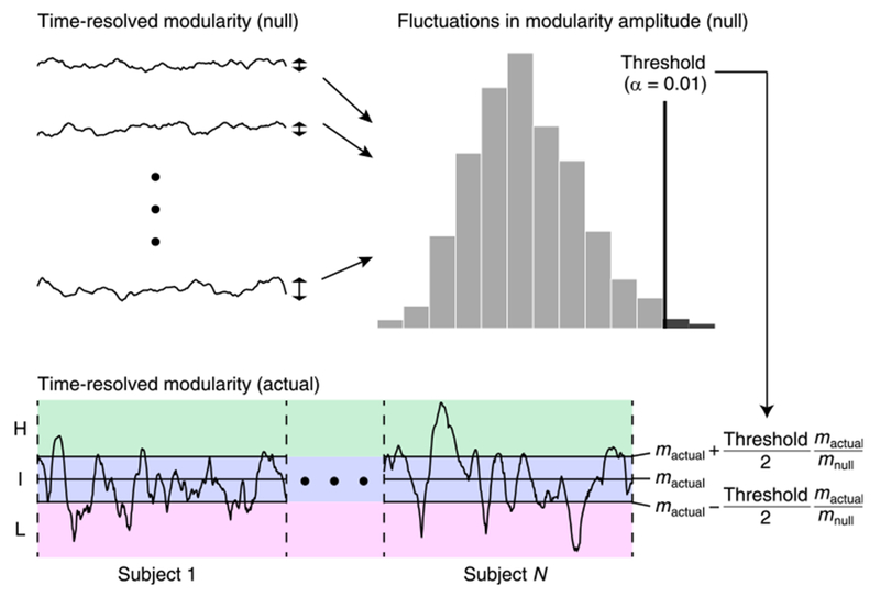
The procedure to determine the high and low modularity periods. Modularity of null time-resolved functional connectivity was generated to obtain null distributions of fluctuations in modularity amplitude. The threshold with α = 0.01 in this null distribution was used for determining periods when actual time-resolved modularity was significantly greater or smaller than its median across subjects m_actual. With this threshold and the normalization constant m_actual/m_null (m_null: the median of time-resolved modularity across all samples from the null distribution), time-resolved functional connectivity in each time window was associated with either the high modularity (H), the intermediate (I) or the low modularity (L) period (also see the paragraph containing Eqs. (2) and (3)).

Null time-resolved functional connectivity was generated using stationary vector autoregressive (VAR) models (Chang and Glover, 2010; Zalesky et al., 2014; de Pasquale et al., 2016; Shine et al., 2016a, b). Parameters in the null stationary VAR models were estimated from actual rs-fMRI time series for each pair of regions. The order of the VAR models was set to 11 (in the HCP dataset) and 12 (in the NKI dataset) to use a maximum lag of approximately 8 s (Zalesky et al., 2014; Shine et al., 2016a). The estimated VAR models were used for individually simulating null stationary rs-fMRI time series for each pair of regions, where initial values for the simulation were a randomly-sampled contiguous block of actual rs-fMRI time series and the innovation term was a randomly-sampled residual of the VAR estimation. From the simulated rs-fMRI data the null time-resolved functional connectivity was computed in the same way as the actual data. As in Zalesky et al. (2014) and Shine et al. (2016a, b), a total of around 2,500 null samples (HCP, 30 samples×84 subjects; NKI, 32 samples×80 subjects) were generated from actual data of all subjects for each rs-fMRI run.

Null distributions of fluctuations in modularity amplitude were obtained from Q_t of null time-resolved functional connectivity. A threshold with α = 0.01 in this null distribution (see Fig. 1) was used to determine the high and low modularity periods. The high modularity period was defined as the period when

$${\mathit{Q}}_{\mathit{t}}>m_{\text{actual}}+\frac{\text{Threshold}}{2}\frac{m_{\text{actual}}}{m_{\text{null}}}$$ (2)

holds, where m_actual and m_null are the median of actual and null time-resolved modularity across all subjects and samples, respectively. Similarly, the low modularity period was defined as the period when

$${\mathit{Q}}_{\mathit{t}}<m_{\text{actual}}-\frac{\text{Threshold}}{2}\frac{m_{\text{actual}}}{m_{\text{null}}}$$ (3)

holds and the intermediate period was the period other than the high or the low modularity period. In Eqs. (2) and (3) we multiplied the threshold by the normalization term m_actual/m_null to absorb potential discrepancies in overall Q_t magnitude between the actual data and the null data generated from the pairwise VAR simulations.

We generated null data from stationary VAR models to determine the periods of high and low modularity because these null models have been used previously in studies by Zalesky et al. (2014) and Shine et al. (2016a, b) that examined fluctuations in network attributes closely related to modularity, i.e. efficiency and the balance of integration and segregation. Our use of VAR models allows a more direct comparison of our own findings with those of these earlier studies. There are other approaches to generate null data, for instance, phase randomization with the same random sequence of phases (Prichard and Theiler, 1994) and generating covariance- and spectra-constrained random normal deviates (Laumann et al., 2016). Recent discussion on the use of null models in time-resolved functional connectivity studies can be found in Liégeois et al. (2017) and Miller et al. (2017).

2.6. Analysis of spatial connectivity patterns

Spatial patterns of time-resolved functional connectivity in the high or the low modularity period were mainly assessed with their temporal median (i.e., the centroid of time-resolved functional connectivity in the high or the low modularity period). These averaged connectivity patterns were characterized by referring to known intrinsic functional connectivity networks (Yeo et al., 2011) as well as by comparing to the connectivity patterns observed in low-dimensional functional connectivity states detected by the k-means clustering algorithm and PCA.

The k-means clustering algorithm has been widely used for detecting a small set of brief functional connectivity patterns (Allen et al., 2014; Damaraju et al., 2014; Barttfeld et al., 2015; Hutchison and Morton, 2015; Gonzalez-Castillo et al., 2015; Rashid et al., 2016; Nomi et al., 2017). We performed k-means clustering using the same procedure as in Allen et al. (2014) and Barttfeld et al. (2015). In this procedure time-resolved functional connectivity concatenated across subjects was subsampled along the time dimension before clustering of all samples. The subsampling was performed by choosing local maxima of the time series of functional connectivity variance, resulting in 15–35 (HCP) and 24–41 (NKI) windows per subjects in subject exemplars. The clustering algorithm was first applied to this set of subject exemplars 500 times with the l1 distance metric and random initialization, and then the obtained median centroids with the minimum error were used as an initial starting point for the subsequent k-means clustering of all time window samples. We used k = 2 as the number of clusters in order to extract two major distinctive connectivity states, and we compared the connectivity patterns observed in their cluster centroids to the patterns found in the centroids of the high and low modularity periods.

Unlike the k-means clustering, PCA has been used to extract a low-dimensional representation of time-resolved functional connectivity in a continuous manner. We performed PCA according to the approach described in Leonardi et al. (2013). The principal components were obtained by eigenvalue decomposition: CC^T = UDU^T, where the matrix C denotes time-resolved functional connectivity concatenated across subjects (here the temporal average of time-resolved connectivity was subtracted individually). The matrix U contains the eigenvectors of CC^T (i.e., the principal components of C) in its columns and D is a diagonal matrix containing the corresponding eigenvalues. The weights of principal components were derived as U^TC, representing the contribution of each principal component in the variability of time-resolved functional connectivity over time. We mainly focused on the principal component with the largest eigenvalue (the first principal component) and compared the connectivity patterns in the first principal component to the patterns observed in differences of centroid edge weights between the high and low modularity periods.

2.7. Analysis of temporal homogeneity

Temporal homogeneity of time-resolved functional connectivity within the high or the low modularity period was evaluated using similarity measures for edge weights and partitions of functional networks. These similarity measures were computed between samples of time-resolved functional connectivity in each modularity period within individuals, as well as between each sample of time-resolved functional connectivity and its corresponding centroid. The similarity of edge weights was quantified by the Pearson correlation coefficient between the vectorized weights. The similarity of partitions was quantified by the normalized mutual information using the BCT function partition_distance.m.

2.8. Analysis of test-retest reliability

Test-retest reliability of the occurrence of the high and low modularity periods within each individual was evaluated using the multi-session rs-fMRI data in the HCP dataset. The occurrence of these periods was assessed through their frequency and mean dwell time (Allen et al., 2014; Damaraju et al., 2014; Hutchison and Morton, 2015). The frequency is defined as the ratio of the number of time windows classified into a particular modularity period relative to the total number of windows. The mean dwell time is the number of consecutive windows classified into a particular modularity period, averaged within each subject. The mean dwell time of a modularity period to which no windows were assigned was set to zero. We omitted the first and last segments of consecutive windows from the mean dwell time since the beginnings and/or the ends of these episodes fall outside of the scanning period. We did not define the mean dwell time of a modularity period in a subject when all its consecutive windows overlapped with either the beginning or the end of the entire scan period.

The test-retest reliability was quantified by the intra-class correlation coefficient (ICC; Shrout and Fleiss, 1979). The ICC has been used in a number of test-retest studies on rs-fMRI data (Schwarz and McGonigle, 2011; Wang et al., 2011; Braun et al., 2012; Guo et al., 2012; Cao et al., 2014a; Andellini et al., 2015; Termenon et al., 2016; for a review, see Zuo and Xing, 2014). We computed the ICC under a two-way mixed model (McGraw and Wong, 1996):

$$\text{ICC}=\frac{\text{BMS}-\text{EMS}}{\text{BMS}+(l-1)\text{EMS}},$$ (4)

where BMS is the between-subjects mean square, EMS is the error mean square and l is the number of repeated observations per subject. According to previous rs-fMRI test-retest studies (Guo et al., 2012; Andellini et al., 2015), we interpreted 0.2<ICC ≤ 0.4 as indicative of a fair test-retest reliability and ICC>0.4 as moderate to good test-retest reliability. Consistent with Braun et al. (2012), Cao et al. (2014a) and Andellini et al. (2015), negative ICC scores were set to zero, since the reason for the presence of negative ICCs is unclear (Müller and Büttner, 1994) and negative reliability is difficult to interpret (Rousson et al., 2002).

3. Results

Most of the results presented in this section (in Figs. 2–5 and Table 2) are derived from run 2LR of the HCP dataset. Reproducibility of the findings about the spatial connectivity patterns and the temporal homogeneity were examined in Supplementary Results using the other three runs of the HCP dataset (and a single run of the NKI dataset). We selected run 2LR because time-resolved modularity Q_t in this run was least affected by head movements; the correlation coefficient between Q_t and the sliding-window-averaged FD, averaged over subjects, was −0.11 in run 1LR, −0.056 in run 1RL, −0.029 in run 2LR and −0.10 in run 2RL. This mean correlation coefficient was also found to be small in the NKI dataset (−0.064). The relationships of Q_t to FD are further evaluated in more detail in Supplementary Results.

3.1. Spatial connectivity patterns

First, we examined spatial patterns of time-resolved functional connectivity averaged within each modularity period. Fig. 2A shows the centroids of the high modularity, the intermediate and the low modularity periods. The centroid of the high modularity period had the highest contrast of edge weights, exhibiting the modular organization of distinct functional networks most clearly. Differences of centroid edge weights between the high and low modularity periods can be characterized as a pronounced dissociation of the task-negative DMN module from the task-positive DAN, VAN, SMN and VIS modules in the high modularity period. These spatial patterns were less evident in the low modularity period, which exhibited much less differentiated (“flat”) connectivity patterns in its centroid. Increased dissociation of the task-positive and task-negative systems in the high modularity period can also be seen in Supplementary Fig. S2, where nodes in the centroids are reordered based on communities detected by modularity maximization in long time-scale functional connectivity.

Fig. 2.

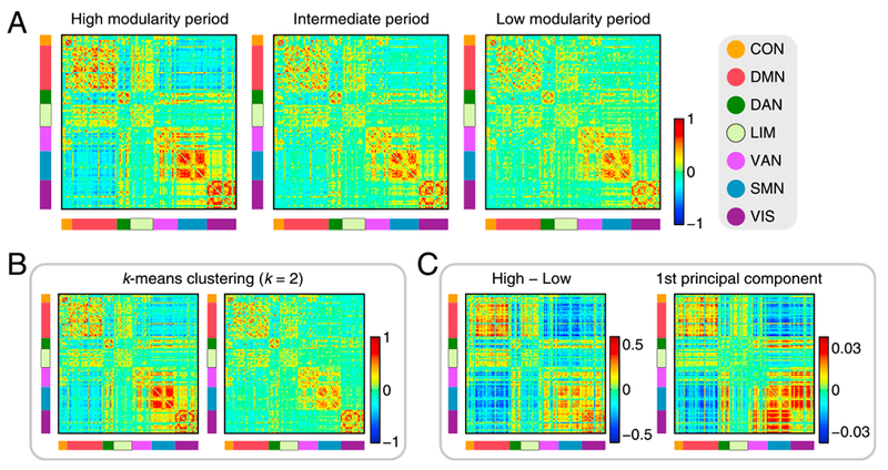
A, Centroids of time-resolved functional connectivity in the high modularity, the intermediate and the low modularity periods. A list of the assignment of cortical nodes to the 7 network components in Yeo et al. (2011) is presented in Supplementary Fig. S1. B, Centroids derived from the k-means clustering algorithm with k = 2. C, Left: differences of centroid edge weights between the high and low modularity periods. Right: the first principal component of time-resolved functional connectivity.

We then compared the connectivity patterns observed in the centroids of the high and low modularity periods to the patterns derived from the k-means clustering algorithm and PCA. Fig. 2B shows that the centroids of the high and low modularity periods had similar connectivity patterns to the patterns observed in the centroids of the two mutually-distinctive connectivity states detected using k-means clustering with k = 2. Differences of centroid edge weights between the high and low modularity periods also resembled the first principal component of time-resolved functional connectivity (see Fig. 2C), indicating that transitions between the high and low modularity periods mainly occurred along the direction of the principal component that explained the largest amount of variance. These results suggest that transitions between the high and low modularity periods, accompanied by changes in the degree of dissociation of the DMN from task-positive networks, accounted for much of the observed fluctuations in time-resolved functional connectivity.

3.2. Temporal homogeneity

Next, we investigated temporal homogeneity of time-resolved functional connectivity within each modularity period. We first looked into the similarity of time-resolved connectivity in a single representative subject. Then, we assessed the similarity of time-resolved connectivity using the data from all subjects.

3.2.1. Individual subject analysis

Fig. 3A displays exemplars of time-resolved functional connectivity in the high and low modularity periods. As in the centroids shown in Fig. 2A, the dissociation of the DMN module from the task-positive network modules was more evident in exemplars sampled from the high modularity period, whereas this module configuration was less pronounced in exemplars sampled from the low modularity period. These exemplars of time-resolved functional connectivity were computed from the time windows whose temporal positions are indicated by the small triangles in the transition sequence of modularity periods shown in Fig. 3B. Fig. 3C shows the matrix displaying the similarity between samples of time-resolved functional connectivity, where the same time axis is used in Fig. 3B and C. This similarity matrix demonstrates that samples of time-resolved functional connectivity in the high modularity period were similar to each other, whereas those in the low modularity period were dissimilar to each other (the similarity of the exemplars presented in Fig. 3A is highlighted by the circles in Fig. 3C).

Fig. 3.

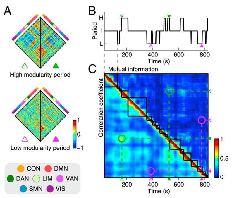
Analysis of temporal homogeneity in one representative subject (subject ID in the HCP database: 133928). A, Exemplars of time-resolved functional connectivity in the high and low modularity periods. B, Transition sequence of modularity periods. The green and magenta triangles are placed at the positions of the time windows from which the exemplars shown in A were computed. C, Similarity between samples of time-resolved functional connectivity. The lower triangular part shows the similarity of edge weights quantified by the Pearson correlation coefficient and the upper triangular part presents the similarity of partitions quantified by the normalized mutual information. The green and magenta circles highlight the similarity scores between the exemplars presented in A.

3.2.2. Group analysis

Fig. 4 shows distributions of the similarity scores over all subjects. Consistent with our observations in the individual subject analysis, samples of time-resolved functional connectivity in the high modularity period were more similar to each other compared to the low modularity periods, in terms of both edge weights (Cohen’s d = 1.4) and partitions (d = 1.2) (see Fig. 4A; the p-values were essentially zero due to a large number of samples in the distributions). The greater similarity in the high modularity period was also confirmed when the similarity scores were computed between each sample of time-resolved functional connectivity and its corresponding centroid, both for edge weights (d = 1.1) and partitions (d = 0.9) (see Fig. 4B). These results indicate that the modular connectivity patterns observed in the high modularity period are relatively homogeneous in time, while the flat connectivity patterns in the low modularity period are relatively heterogeneous.

Fig. 4.

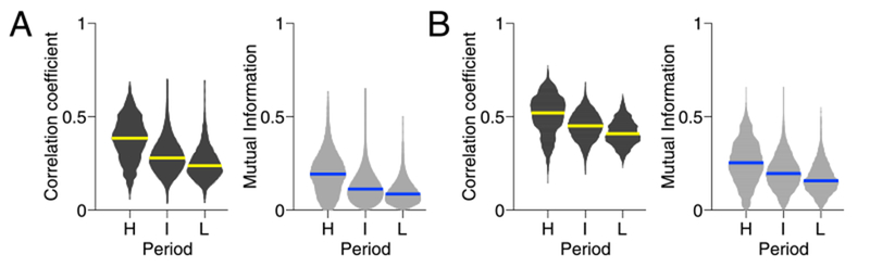
Distributions of the similarity measures of time-resolved functional connectivity. A bar in a distribution indicates the median. A, The similarity of edge weights (left; Pearson correlation coefficient) and partitions (right; normalized mutual information) between samples of time-resolved functional connectivity in each modularity period within individuals. These distributions were derived only from pairs of samples that are apart from each other by more than the width of the time window. B, The similarity of edge weights (left) and partitions (right) between each sample of time-resolved functional connectivity and its corresponding centroid.

The correlation coefficients displayed in Fig. 4B are projected into the space spanned by the first and second principal components (PCs 1 and 2) in Fig. 5 (left panels). In this figure each colored dot represents a sample of time-resolved functional connectivity and its color indicates the similarity to its corresponding centroid. The color gradient in this figure shows that the greater similarity to respective centroids was associated with a larger weight of PC 1, which corresponds to a greater expression of the modular connectivity patterns in Fig. 2C (right) in each sample. Although the cluster of samples in the high modularity period partially overlapped with the cluster of the low modularity period, their centers of mass were separated along the direction of PC 1 (see Fig. 5, right panels), as is expected from the similarity of connectivity patterns between PC 1 and the differences of centroid edge weights (see Fig. 2C).

Fig. 5.

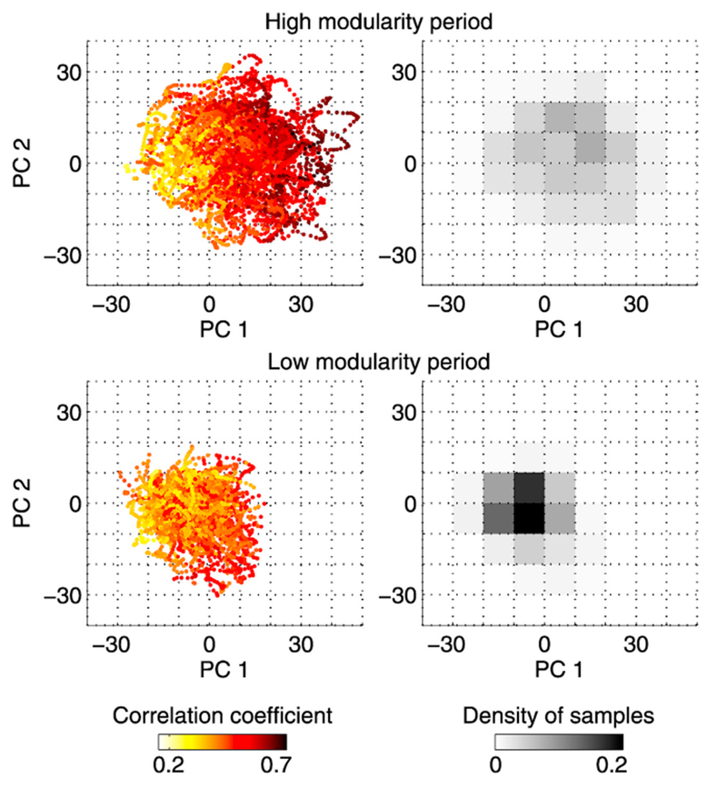
Left panels: samples of time-resolved functional connectivity in the space spanned by the first and second principal components (PCs 1 and 2). Each colored dot represents a sample of time-resolved functional connectivity and its color shows the similarity (Pearson correlation coefficient) of edge weights to its corresponding centroid. The numbers of samples in the high and low modularity periods were almost the same (5,329 and 5,310, respectively). Right panels: two-dimensional histograms showing the density of samples of time-resolved functional connectivity in the PC space.

It should be mentioned that the homogeneity of time-resolved functional connectivity is not necessarily linked to the cohesion of samples in the PC space. On the contrary, relatively homogeneous samples in the high modularity period were not well clustered but rather dispersed, while relatively heterogeneous samples in the low modularity period were more densely clustered near the origin of the PC space (see Fig. 5). This is because, in the low modularity period, a variety of combinations of components other than PC 1 or PC 2 shaped heterogeneous connectivity patterns across the clustered samples near the origin. On the other hand, dispersions to the positive direction of PC 1 resulted in an increased homogeneity of samples in the high modularity period, since its centroid and PC 1 shared similar connectivity patterns as presented in Fig. 2.

3.3. Test-retest reliability

Finally, we evaluated the test-retest reliability of the occurrence of each modularity period within individuals. We first confirmed that the occurrence of the modularity periods varied across individuals in run 2LR; the ranges of the frequency across subjects were 0-0.49 (H), 0.28–0.91 (I) and 0.0054–0.72 (L); and the ranges of the mean dwell time were 0–62 s (H), 26–114 s (I) and 3.6–72 s (L). The following test-retest analysis examined how consistently each modularity period appeared within individuals over the two sessions (2 × 28 min) and the four runs (4 × 14 min) of rs-fMRI scans in the HCP dataset.

Table 1 displays the ICC of the frequency and mean dwell time of each modularity period. Moderate session-level reliability (ICC > 0.4) was observed in the frequency of the high and low modularity periods as well as the mean dwell time of the low modularity period. These metrics of occurrence also demonstrated fair (ICC >0.2) to moderate run-level reliability, while the dwell time of the high modularity period demonstrated only fair session-level reliability. The frequency and mean dwell time of the intermediate period were not reproducible both at the session and run levels. Our test-retest analysis showed that the individual differences in the occurrence of the high and low modularity periods were somewhat reproducible.

Table 1.

The ICCs of the frequency and mean dwell time of each modularity period and the ICC of the modularity Q of long-timescale functional connectivity.

	High modularity period		Intermediate period		Low modularity period		Modularity Q
	Frequency	Dwell time	Frequency	Dwell time	Frequency	Dwell time
Across two sessions (one session: 28 min)
ICC	0.44	0.21	0.19	0	0.52	0.55	0.46
95% CI	[0.25, 0.59]	[0.00, 0.41]	[0, 0.38]	[0, 0.10]	[0.34, 0.66]	[0.39, 0.69]	[0.27, 0.61]
Across four runs (one run: 14 min)
ICC	0.28	0.11	0.16	0	0.42	0.31	0.45
95% CI	[0.17, 0.40]	[0.01, 0.22]	[0.06, 0.28]	[0, 0.08]	[0.30, 0.53]	[0.20, 0.44]	[0.33, 0.56]

ICC >0.4 is shown in bold and 0.2< ICC ≤ 0.4 is shown in bold italic. As explained in the section entitled Analysis of test-retest reliability, negative ICC scores are regarded as zero.

The individual differences in the occurrence of the high and low modularity periods were closely linked to the previously-reported individual differences in the modularity Q of long-timescale functional connectivity. Consistent with the literature, we observed that the long-timescale modularity Q varied across individuals (the range of Q across subjects in run 2LR, 0.37–0.64) with moderate session-level and run-level reproducibility (see Table 1). Table 2 shows that Q was positively (respectively, negatively) correlated to the frequency and mean dwell time of the high (respectively, low) modularity period across individuals, indicating that the high (low) modular period is more likely to occur and lasts with a longer duration in individuals with high (low) Q scores. This result demonstrated that the individual variations in the modularity Q of long-timescale functional connectivity can be explained by the differences in the occurrence of the high and low modularity periods across individuals.

Table 2.

Pearson correlation coefficient between the modularity Q of long-timescale functional connectivity and the frequency and mean dwell time of each modularity period (bold, p<0.01).

	High modularity state		Intermediate state		Low modularity state
	Frequency	Dwell time	Frequency	Dwell time	Frequency	Dwell time
r	0.65	0.35	0.13	−0.03	−0.65	−0.49
95% CI	[0.50, 0.76]	[0.14, 0.52]	[−0.08, 0.34]	[−0.24, 0.19]	[−0.76, −0.50]	[−0.64, −0.31]

4. Discussion

Although recent studies have reported that fluctuations in edge weights and topology of resting-state functional brain networks co-occur with temporal changes in their modularity, the spatiotemporal configurations of time-resolved functional networks during periods of high and low modularity have remained largely unexplored. In this study we examined how time-resolved functional networks sampled from periods of high and low modularity are organized in space and time, whether the occurrence of these periods varies across individuals, and whether individual differences are reproducible across sessions. Our analysis of spatial connectivity patterns showed that the time-resolved connectivity in the high modularity period was characterized by the pronounced dissociation of the DMN from task-positive networks and that the transitions between this module structure and the flat connectivity profiles of the low modularity period well summarized overall fluctuations of the time-resolved connectivity. The temporal homogeneity analysis demonstrated that the decoupling of the DMN from task-positive networks consistently occurred across samples of the time-resolved connectivity in the high modularity period, whereas the flat connectivity patterns observed in the low modularity period were relatively heterogeneous and more dissimilar to each other over time. The test-retest analysis confirmed that the occurrence of the high and low modularity periods varied across individuals with moderate inter-session reproducibility and that these variations across individuals can explain individual differences in the modularity of long-timescale functional connectivity.

Our spatial and temporal analyses of time-resolved functional networks in the high and low modularity periods bring a new perspective to previously observed attributes of the correlation structure in rs-fMRI data. It is well-established that time courses of regional activity in the DMN and task-positive networks are correlated within and anti-correlated between networks when these correlations are computed from several minutes of rs-fMRI measurements (Fox et al., 2005; Fox and Raichle, 2007). Our findings on a time scale of tens of seconds demonstrated that this specific correlation structure among the DMN and task-positive networks was recurrently strengthened in the high modularity period, whereas this structure was weakened and was broken down heterogeneously in the low modularity period. Temporal fluctuations in expression of this specific correlation structure have already been reported in recent studies (e.g., Allen et al., 2014; Betzel et al., 2016). In the present paper we demonstrate a link of this structure to variations in the temporal homogeneity (or heterogeneity) of short-timescale correlations. Our results suggest that the canonical long-timescale correlation structure in rs-fMRI data is shaped by the repeated appearance of relatively uniform correlation patterns in the high modularity period and an averaging out of many dissimilar correlation patterns in the low modularity period. From this perspective, one can argue that the proportion of the high to the low modularity period in rs-fMRI data may underlie the degree to which the DMN is decoupled from task-positive networks in estimates of long-timescale correlations.

The findings about the spatial and temporal connectivity profiles in the high and low modularity periods also provide another perspective on segregated and integrated states of time-resolved functional networks, recently studied by Shine et al. (2016a). There is growing interest in temporal fluctuations in the balance between segregation and integration of neural information (Sporns, 2013; Deco et al., 2015). Shine and colleagues defined states of segregation and integration based on patterns in nodal participation coefficients and within-module degree of time-resolved functional networks and demonstrated that topology of the time-resolved networks in the segregated and integrated states was associated with high and low modularity, respectively (Shine et al., 2016a). Importantly, alternations between these segregated and integrated states were related to cognitive function and the activity of neuromodulatory systems—a network attribute for integration was found to be correlated with measures quantifying fast and effective cognitive performance and with increases in pupil diameter as a surrogate measure of arousal (Shine et al., 2016a). We found that the dissociation of the DMN from task-positive networks was diminished and the similarity between samples of time-resolved functional connectivity was decreased in the low modularity period—hallmarks of network organization that may indeed be related to the level of functional integration. These results suggest that efficient cognitive processing in the integrated state is likely to be supported by multiple, heterogeneous coupling patterns across the whole brain, accompanied by dynamic reconfiguration of interactions between the DMN and other networks, as seen with greater task demands of working memory (Vatansever et al., 2015).

The test-retest analysis of the high and low modularity periods offers a new interpretation of individual differences in modularity measured over longer timescales. Previous studies have shown that this long-timescale modularity varies across individuals and its variability is associated with life-span development and aging (Cao et al., 2014b; Chan et al., 2014), and working memory performance (Stevens et al., 2012; Meunier et al., 2014; Stanley et al., 2014). In this study we demonstrated that individual variations in long-timescale modularity are related to variations in the occurrence of high- and low-modularity periods, after confirming their moderate session-level test-retest reliability. The greater occurrence of the high (low) modularity period in individuals with higher (lower) long-timescale modularity itself is not surprising given their definition; however, it provides a way to trace individual variations in long-timescale modularity to the variable occurrence of temporal building blocks at shorter time scales. The relationship established in our test-retest analysis indicates that individual variations in long-timescale modularity can be interpreted as a result of variations in the emergence of network properties specific to either the high or the low modularity period in time-resolved functional connectivity. The demographic and behavioral relevance of long-timescale modularity may therefore be rooted in the differences in the propensity of the DMN to associate with task-positive networks, and in the balance between homogeneity and heterogeneity of time-resolved functional connectivity.

There are several methodological limitations in this study. First, the sliding window approach is a simple and the most commonly used method for computing time-resolved functional connectivity (Hutchison et al., 2013a; Preti et al., 2017), but it has limitations in detecting sharp connectivity transitions (Lindquist et al., 2014; Shine et al., 2015; Shakil et al., 2016). Since it is necessary to set the width of the time window to be longer than or equal to the reciprocal of the lowest frequency of rs-fMRI data to suppress spurious connectivity fluctuations (Leonardi and Van De Ville, 2015; Zalesky and Breakspear, 2015), changes faster than this specific temporal scale cannot be captured with this approach. This highlights the need to establish methods that can handle connectivity fluctuations on multiple time scales. Second, community detection by modularity maximization fails to detect communities below a certain scale under certain conditions (the resolution limit; Fortunato and Barthelemy, 2007). A single default resolution parameter is used throughout this paper to properly compare the modularity quality function; however, this prevents the algorithm from detecting communities of different sizes. A possible strategy to circumvent this issue is to explore a range of resolution parameters to reveal multiscale community structure in networks (Betzel et al., 2013). Third, head movements are a potential confound in rs-fMRI data (Power et al., 2012, 2014). To solve this issue, we employed extensive artifact reduction methods in this study; high motion subjects were discarded; artifactual BOLD time points were censored and interpolated; motion estimates and the global, white matter and CSF mean signals were regressed out. It should be noted that the findings presented in Results (other than in the section Test-retest reliability) were derived from the rs-fMRI run least affected by head movements, and that there was no consistent relation between the head movements and the modularity time series in this run (see Supplementary Results). And fourth, images in the HCP and the NKI datasets were independently preprocessed. Nevertheless, the findings in this study (with the exception of the test-retest analysis; the NKI dataset contained only a single rs-fMRI run) were reproducible across the HCP and the NKI datasets (see Supplementary Results). While there were some minor differences in the spatial connectivity patterns and the temporal homogeneity (see Supplementary Results), they did not alter the conclusions of this study.

Future research is needed to draw firm conclusions about specific neurobiological mechanisms that underlie fluctuations in the modularity of time-resolved functional networks. For a better understanding of these mechanisms, it is particularly important to establish the relationship of dynamic fluctuations in modularity to their underlying structural connectivity. A simple approach to relate to the structure is evaluating the similarity between structural and time-resolved functional connectivity (Barttfeld et al., 2015; Liégeois et al., 2016). This approach can be used to determine in which modularity period time-resolved functional networks are more shaped by structural connectivity. Another promising approach is to simulate fluctuations in modular organization of resting-state functional networks using whole-brain computational models constrained by structural connectivity (Hansen et al., 2015; Ponce-Alvarez et al., 2015). Generative processes of the modularity fluctuations can be studied by manipulating elements in these models and examining its effects on the simulated time-resolved module configuration. Examining individual differences is also an important direction to relate the modularity fluctuations to the underlying structure. Future analyses integrating individual variations in the occurrence of the high and low modularity periods and structural connectivity, in addition to demographics and cognitive performance, may contribute to a more comprehensive understanding of fluctuations in the modularity of time-resolved functional networks.

References

- Allen EA, Damaraju E, Plis SM, Erhardt EB, Eichele T, Calhoun VD, 2014. Tracking whole-brain connectivity dynamics in the resting state. Cereb. Cortex 24, 663–676. [DOI] [PMC free article] [PubMed] [Google Scholar]
- Andellini M, Cannatà V, Gazzellini S, Bernardi B, Napolitano A, 2015. Test-retest reliability of graph metrics of resting state MRI functional brain networks: a review. J. Neurosci. Methods 253, 183–192. [DOI] [PubMed] [Google Scholar]
- Baker AP, Brookes MJ, Rezek IA, Smith SM, Behrens TEJ, Probert Smith PJ, Woolrich MW, 2014. Fast transient networks in spontaneous human brain activity. eLife 3, e01867. [DOI] [PMC free article] [PubMed] [Google Scholar]
- Barttfeld P, Uhrig L, Sitt JD, Sigman M, Jarraya B, Dehaene S, 2015. Signature of consciousness in the dynamics of resting-state brain activity. Proc. Natl. Acad. Sci. U. S. A. 112, 887–892. [DOI] [PMC free article] [PubMed] [Google Scholar]
- Bassett DS, Wymbs NF, Porter MA, Mucha PJ, Carlson JM, Grafton ST, 2011. Dynamic reconfiguration of human brain networks during learning. Proc. Natl. Acad. Sci. U. S. A. 108, 7641–7646. [DOI] [PMC free article] [PubMed] [Google Scholar]
- Betzel RF, Byrge L, He Y, Goñi J, Zuo XN, Sporns O, 2014. Changes in structural and functional connectivity among resting-state networks across the human lifespan. NeuroImage 102, 345–357. [DOI] [PubMed] [Google Scholar]
- Betzel RF, Fukushima M, He Y, Zuo XN, Sporns O, 2016. Dynamic fluctuations coincide with periods of high and low modularity in resting-state functional brain networks. NeuroImage 127, 287–297. [DOI] [PMC free article] [PubMed] [Google Scholar]
- Betzel RF, Griffa A, Avena-Koenigsberger A, Goñi J, Thiran JP, Hagmann P, Sporns O, 2013. Multi-scale community organization of the human structural connectome and its relationship with resting-state functional connectivity. Netw. Sci. 1, 353–373. [Google Scholar]
- Biswal B, Yetkin FZ, Haughton VM, Hyde JS, 1995. Functional connectivity in the motor cortex of resting human brain using echo-planar MRI. Magn. Reson. Med. 34, 537–541. [DOI] [PubMed] [Google Scholar]
- Blondel VD, Guillaume JL, Lambiotte R, Lefebvre E, 2008. Fast unfolding of communities in large networks. J. Stat. Mech. Theor. Exp. 2008, P10008. [Google Scholar]
- Braun U, Plichta MM, Esslinger C, Sauer C, Haddad L, Grimm O, Mier D, Mohnke S, Heinz A, Erk S, Walter H, Seiferth N, Kirsch P, Meyer-Lindenberg A, 2012. Test-retest reliability of resting-state connectivity network characteristics using fMRI and graph theoretical measures. NeuroImage 59, 1404–1412. [DOI] [PubMed] [Google Scholar]
- Braun U, Schäfer A, Walter H, Erk S, Romanczuk-Seiferth N, Haddad L, Schweiger JI, Grimm O, Heinz A, Tost H, Meyer-Lindenberg A, Bassett DS, 2015. Dynamic reconfiguration of frontal brain networks during executive cognition in humans. Proc. Natl. Acad. Sci. U. S. A. 112, 11678–11683. [DOI] [PMC free article] [PubMed] [Google Scholar]
- Brookes MJ, O’Neill GC, Hall EL, Woolrich MW, Baker A, Palazzo Corner S, Robson SE, Morris PG, Barnes GR, 2014. Measuring temporal, spectral and spatial changes in electrophysiological brain network connectivity. NeuroImage 91C, 282–299. [DOI] [PubMed] [Google Scholar]
- Brookes MJ, Woolrich MW, Luckhoo H, Price D, Hale JR, Stephenson MC, Barnes GR, Smith SM, Morris PG, 2011. Investigating the electrophysiological basis of resting state networks using magnetoencephalography. Proc. Natl. Acad. Sci. U. S. A. 108, 16783–16788. [DOI] [PMC free article] [PubMed] [Google Scholar]
- Buckner RL, Sepulcre J, Talukdar T, Krienen FM, Liu H, Hedden T, Andrews-Hanna JR, Sperling RA, Johnson KA, 2009. Cortical hubs revealed by intrinsic functional connectivity: mapping, assessment of stability, and relation to Alzheimer’s disease. J. Neurosci. 29, 1860–1873. [DOI] [PMC free article] [PubMed] [Google Scholar]
- Bullmore ET, Sporns O, 2009. Complex brain networks: graph theoretical analysis of structural and functional systems. Nat. Rev. Neurosci. 10, 186–198. [DOI] [PubMed] [Google Scholar]
- Bullmore ET, Sporns O, 2012. The economy of brain network organization. Nat. Rev. Neurosci. 13, 336–349. [DOI] [PubMed] [Google Scholar]
- Calhoun VD, Miller R, Pearlson G, Adalı T, 2014. The chronnectome: time-varying connectivity networks as the next frontier in fMRI data discovery. Neuron 84, 262–274. [DOI] [PMC free article] [PubMed] [Google Scholar]
- Cammoun L, Gigandet X, Meskaldji D, Thiran JP, Sporns O, Do KQ, Maeder P, Meuli R, Hagmann P, 2012. Mapping the human connectome at multiple scales with diffusion spectrum MRI. J. Neurosci. Methods 203, 386–397. [DOI] [PubMed] [Google Scholar]
- Cao H, Plichta MM, Schäfer A, Haddad L, Grimm O, Schneider M, Esslinger C, Kirsch P, Meyer-Lindenberg A, Tost H, 2014a. Test-retest reliability of fMRI-based graph theoretical properties during working memory, emotion processing, and resting state. NeuroImage 84, 888–900. [DOI] [PubMed] [Google Scholar]
- Cao M, Wang JH, Dai ZJ, Cao XY, Jiang LL, Fan FM, Song XW, Xia MR, Shu N, Dong Q, Milham MP, Castellanos FX, Zuo XN, He Y, 2014b. Topological organization of the human brain functional connectome across the lifespan. Dev. Cogn. Neurosci. 7, 76–93. [DOI] [PMC free article] [PubMed] [Google Scholar]
- Chan MY, Park DC, Savalia NK, Petersen SE, Wig GS, 2014. Decreased segregation of brain systems across the healthy adult lifespan. Proc. Natl. Acad. Sci. U. S. A. 111, E4997–E5006. [DOI] [PMC free article] [PubMed] [Google Scholar]
- Chang C, Glover GH, 2010. Time-frequency dynamics of resting-state brain connectivity measured with fMRI. NeuroImage 50, 81–98. [DOI] [PMC free article] [PubMed] [Google Scholar]
- Chen T, Cai W, Ryali S, Supekar K, Menon V, 2016. Distinct global brain dynamics and spatiotemporal organization of the salience network. PLoS Biol. 14, e1002469. [DOI] [PMC free article] [PubMed] [Google Scholar]
- Clune J, Mouret JB, Lipson H, 2013. The evolutionary origins of modularity. Proc. Biol. Sci. 280, 20122863. [DOI] [PMC free article] [PubMed] [Google Scholar]
- Cox RW, 2012. AFNI: what a long strange trip it’s been. NeuroImage 62, 743–747. [DOI] [PMC free article] [PubMed] [Google Scholar]
- Damaraju E, Allen EA, Belger A, Ford JM, McEwen S, Mathalon DH, Mueller BA, Pearlson GD, Potkin SG, Preda A, Turner JA, Vaidya JG, van Erp TG, Calhoun VD, 2014. Dynamic functional connectivity analysis reveals transient states of dysconnectivity in schizophrenia. NeuroImage Clin. 5, 298–308. [DOI] [PMC free article] [PubMed] [Google Scholar]
- Damoiseaux JS, Rombouts SARB, Barkhof F, Scheltens P, Stam CJ, Smith SM, Beckmann CF, 2006. Consistent resting-state networks across healthy subjects. Proc. Natl. Acad. Sci. U. S. A. 103, 13848–13853. [DOI] [PMC free article] [PubMed] [Google Scholar]
- de Pasquale F, Della Penna S, Snyder AZ, Lewis C, Mantini D, Marzetti L, Belardinelli P, Ciancetta L, Pizzella V, Romani GL, Corbetta M, 2010. Temporal dynamics of spontaneous MEG activity in brain networks. Proc. Natl. Acad. Sci. U. S. A. 107, 6040–6045. [DOI] [PMC free article] [PubMed] [Google Scholar]
- de Pasquale F, Della Penna S, Snyder AZ, Marzetti L, Pizzella V, Romani GL, Corbetta M, 2012. A cortical core for dynamic integration of functional networks in the resting human brain. Neuron 74, 753–764. [DOI] [PMC free article] [PubMed] [Google Scholar]
- de Pasquale F, Della Penna S, Sporns O, Romani GL, Corbetta M, 2016. A dynamic core network and global efficiency in the resting human brain. Cereb. Cortex 26, 4015–4033. [DOI] [PMC free article] [PubMed] [Google Scholar]
- Deco G, Tononi G, Boly M, Kringelbach ML, 2015. Rethinking segregation and integration: contributions of whole-brain modelling. Nat. Rev. Neurosci. 16, 430–439. [DOI] [PubMed] [Google Scholar]
- Fortunato S, Barthelemy M, 2007. Resolution limit in community detection. Proc. Natl. Acad. Sci. U. S. A. 104, 36–41. [DOI] [PMC free article] [PubMed] [Google Scholar]
- Fox MD, Raichle ME, 2007. Spontaneous fluctuations in brain activity observed with functional magnetic resonance imaging. Nat. Rev. Neurosci. 8, 700–711. [DOI] [PubMed] [Google Scholar]
- Fox MD, Snyder AZ, Vincent JL, Corbetta M, Van Essen DC, Raichle ME, 2005. The human brain is intrinsically organized into dynamic, anticorrelated functional networks. Proc. Natl. Acad. Sci. U. S. A. 102, 9673–9678. [DOI] [PMC free article] [PubMed] [Google Scholar]
- Friston KJ, Williams S, Howard R, Frackowiak RS, Turner R, 1996. Movement-related effects in fMRI time-series. Magn. Reson. Med. 35, 346–355. [DOI] [PubMed] [Google Scholar]
- Gallen CL, Turner GR, Adnan A, D’Esposito M, 2016. Reconfiguration of brain network architecture to support executive control in aging. Neurobiol. Aging 44, 42–52. [DOI] [PMC free article] [PubMed] [Google Scholar]
- Geerligs L, Renken RJ, Saliasi E, Maurits NM, Lorist MM, 2015. A brain-wide study of age-related changes in functional connectivity. Cereb. Cortex 25, 1987–1999. [DOI] [PubMed] [Google Scholar]
- Glasser MF, Sotiropoulos SN, Wilson JA, Coalson TS, Fischl B, Andersson JL, Xu J, Jbabdi S, Webster M, Polimeni JR, Van Essen DC, Jenkinson M, for the WU-Minn HCP Consortium, 2013. The minimal preprocessing pipelines for the Human Connectome Project. NeuroImage 80, 105–124. [DOI] [PMC free article] [PubMed] [Google Scholar]
- Gonzalez-Castillo J, Handwerker DA, Robinson ME, Hoy CW, Buchanan LC, Saad ZS, Bandettini PA, 2014. The spatial structure of resting state connectivity stability on the scale of minutes. Front. Neurosci. 8, 138. [DOI] [PMC free article] [PubMed] [Google Scholar]
- Gonzalez-Castillo J, Hoy CW, Handwerker DA, Robinson ME, Buchanan LC, Saad ZS, Bandettini PA, 2015. Tracking ongoing cognition in individuals using brief, whole-brain functional connectivity patterns. Proc. Natl. Acad. Sci. U. S. A. 112, 8762–8767. [DOI] [PMC free article] [PubMed] [Google Scholar]
- Good BH, de Montjoye YA, Clauset A, 2010. Performance of modularity maximization in practical contexts. Phys. Rev. E 81, 046106. [DOI] [PubMed] [Google Scholar]
- Greicius MD, Srivastava G, Reiss AL, Menon V, 2004. Default-mode network activity distinguishes Alzheimer’s disease from healthy aging: evidence from functional MRI. Proc. Natl. Acad. Sci. U. S. A. 101, 4637–4642. [DOI] [PMC free article] [PubMed] [Google Scholar]
- Guimerà R, Nunes Amaral LA, 2005. Functional cartography of complex metabolic networks. Nature 433, 895–900. [DOI] [PMC free article] [PubMed] [Google Scholar]
- Guo CC, Kurth F, Zhou J, Mayer EA, Eickhoff SB, Kramer JH, Seeley WW, 2012. One-year test-retest reliability of intrinsic connectivity network fMRI in older adults. NeuroImage 61, 1471–1483. [DOI] [PMC free article] [PubMed] [Google Scholar]
- Hagmann P, Cammoun L, Gigandet X, Meuli R, Honey CJ, Wedeen VJ, Sporns O, 2008. Mapping the structural core of human cerebral cortex. PLoS Biol. 6, e159. [DOI] [PMC free article] [PubMed] [Google Scholar]
- Handwerker DA, Roopchansingh V, Gonzalez-Castillo J, Bandettini PA, 2012. Periodic changes in fMRI connectivity. NeuroImage 63, 1712–1719. [DOI] [PMC free article] [PubMed] [Google Scholar]
- Hansen ECA, Battaglia D, Spiegler A, Deco G, Jirsa VK, 2015. Functional connectivity dynamics: modeling the switching behavior of the resting state. NeuroImage 105, 525–535. [DOI] [PubMed] [Google Scholar]
- Hipp JF, Hawellek DJ, Corbetta M, Siegel M, Engel AK, 2012. Large-scale cortical correlation structure of spontaneous oscillatory activity. Nat. Neurosci. 15, 884–892. [DOI] [PMC free article] [PubMed] [Google Scholar]
- Hutchison RM, Morton JB, 2015. Tracking the brain’s functional coupling dynamics over development. J. Neurosci. 35, 6849–6859. [DOI] [PMC free article] [PubMed] [Google Scholar]
- Hutchison RM, Womelsdorf T, Allen EA, Bandettini PA, Calhoun VD, Corbetta M, Della Penna S, Duyn JH, Glover GH, Gonzalez-Castillo J, Handwerker DA, Keilholz S, Kiviniemi V, Leopold DA, de Pasquale F, Sporns O, Walter M, Chang C, 2013a. Dynamic functional connectivity: promise, issues, and interpretations. NeuroImage 80, 360–378. [DOI] [PMC free article] [PubMed] [Google Scholar]
- Hutchison RM, Womelsdorf T, Gati JS, Everling S, Menon RS, 2013b. Resting-state networks show dynamic functional connectivity in awake humans and anesthetized macaques. Hum. Brain Mapp. 34, 2154–2177. [DOI] [PMC free article] [PubMed] [Google Scholar]
- Jones DT, Vemuri P, Murphy MC, Gunter JL, Senjem ML, Machulda MM, Przybelski SA, Gregg BE, Kantarci K, Knopman DS, Boeve BF, Petersen RC, Jack CR, 2012. Non-stationarity in the “resting brain’s” modular architecture. PLoS One 7, e39731. [DOI] [PMC free article] [PubMed] [Google Scholar]
- Kashtan N, Alon U, 2005. Spontaneous evolution of modularity and network motifs. Proc. Natl. Acad. Sci. U. S. A. 102, 13773–13778. [DOI] [PMC free article] [PubMed] [Google Scholar]
- Kashtan N, Noor E, Alon U, 2007. Varying environments can speed up evolution. Proc. Natl. Acad. Sci. U. S. A. 104, 13711–13716. [DOI] [PMC free article] [PubMed] [Google Scholar]
- Keilholz SD, Magnuson ME, Pan WJ, Willis M, Thompson GJ, 2013. Dynamic properties of functional connectivity in the rodent. Brain Connect. 3, 31–40. [DOI] [PMC free article] [PubMed] [Google Scholar]
- Kitzbichler MG, Henson RNA, Smith ML, Nathan PJ, Bullmore ET, 2011. Cognitive effort drives workspace configuration of human brain functional networks. J. Neurosci. 31, 8259–8270. [DOI] [PMC free article] [PubMed] [Google Scholar]
- Kucyi A, Davis KD, 2014. Dynamic functional connectivity of the default mode network tracks daydreaming. NeuroImage 100, 471–480. [DOI] [PubMed] [Google Scholar]
- Laumann TO, Snyder AZ, Mitra AM, Gordon EM, Gratton C, Adeyemo B, Gilmore AW, Nelson SM, Berg JJ, Greene DJ, McCarthy JE, Tagliazucchi E, Laufs H, Schlaggar BL, Dosenbach NUF, Petersen SE, 2016. On the stability of BOLD fMRI correlations. Cereb. Cortex. 10.1093/cercor/bhw265. [DOI] [PMC free article] [PubMed] [Google Scholar]
- Leonardi N, Richiardi J, Gschwind M, Simioni S, Annoni JM, Schluep M, Vuilleumier P, Van De Ville D, 2013. Principal components of functional connectivity: a new approach to study dynamic brain connectivity during rest. NeuroImage 83, 937–950. [DOI] [PubMed] [Google Scholar]
- Leonardi N, Shirer WR, Greicius MD, Van De Ville D, 2014. Disentangling dynamic networks: separated and joint expressions of functional connectivity patterns in time. Hum. Brain Mapp. 35, 5984–5995. [DOI] [PMC free article] [PubMed] [Google Scholar]
- Leonardi N, Van De Ville D, 2015. On spurious and real fluctuations of dynamic functional connectivity during rest. NeuroImage 104, 430–436. [DOI] [PubMed] [Google Scholar]
- Liégeois R, Laumann TO, Snyder AZ, Zhou HJ, Yeo BTT, 2017. Interpreting temporal fluctuations in resting-state functional connectivity MRI. bioRxiv. 10.1101/135681. [DOI] [PubMed] [Google Scholar]
- Liégeois R, Ziegler E, Phillips C, Geurts P, Gómez F, Bahri MA, Yeo BTT, Soddu A, Vanhaudenhuyse A, Laureys S, Sepulchre R, 2016. Cerebral functional connectivity periodically (de)synchronizes with anatomical constraints. Brain Struct. Func. 221, 2985–2997. [DOI] [PubMed] [Google Scholar]
- Lindquist MA, Xu Y, Nebel MB, Caffo BS, 2014. Evaluating dynamic bivariate correlations in resting-state fMRI: a comparison study and a new approach. NeuroImage 101, 531–546. [DOI] [PMC free article] [PubMed] [Google Scholar]
- Madhyastha TM, Askren MK, Boord P, Grabowski TJ, 2015. Dynamic connectivity at rest predicts attention task performance. Brain Connect. 5, 45–59. [DOI] [PMC free article] [PubMed] [Google Scholar]
- McGraw KO, Wong SP, 1996. Forming inferences about some intraclass correlation coefficients. Psychol. Methods 1, 30–46. [Google Scholar]
- Meunier D, Fonlupt P, Saive AL, Plailly J, Ravel N, Royet JP, 2014. Modular structure of functional networks in olfactory memory. NeuroImage 95, 264–275. [DOI] [PubMed] [Google Scholar]
- Meunier D, Lambiotte R, Fornito A, Ersche KD, Bullmore ET, 2009. Hierarchical modularity in human brain functional networks. Front. Hum. Neurosci. 3, 37. [DOI] [PMC free article] [PubMed] [Google Scholar]
- Miller RL, Adalı T, Levin-Schwartz Y, Calhoun VD, 2017. Resting-state fMRI dynamics and null models: perspectives, sampling variability, and simulations. bioRxiv. 10.1101/153411. [DOI] [PMC free article] [PubMed] [Google Scholar]
- Miller RL, Yaesoubi M, Turner JA, Mathalon D, Preda A, Pearlson G, Adalı T, Calhoun VD, 2016. Higher dimensional meta-state analysis reveals reduced resting fMRI connectivity dynamism in schizophrenia patients. PLoS One 11, e0149849. [DOI] [PMC free article] [PubMed] [Google Scholar]
- Müller R, Büttner P, 1994. A critical discussion of intraclass correlation coefficients. Stat. Med. 13, 2465–2476. [DOI] [PubMed] [Google Scholar]
- Newman MEJ, Girvan M, 2004. Finding and evaluating community structure in networks. Phys. Rev. E 69, 026113. [DOI] [PubMed] [Google Scholar]
- Nomi JS, Vij SG, Dajani DR, Steimke R, Damaraju E, Rachakonda S, Calhoun VD, Uddin LQ, 2017. Chronnectomic patterns and neural flexibility underlie executive function. NeuroImage 147, 861–871. [DOI] [PMC free article] [PubMed] [Google Scholar]
- Ponce-Alvarez A, Deco G, Hagmann P, Romani GL, Mantini D, Corbetta M, 2015. Resting-state temporal synchronization networks emerge from connectivity topology and heterogeneity. PLoS Comput. Biol. 11, e1004100. [DOI] [PMC free article] [PubMed] [Google Scholar]
- Power JD, Barnes KA, Snyder AZ, Schlaggar BL, Petersen SE, 2012. Spurious but systematic correlations in functional connectivity MRI networks arise from subject motion. NeuroImage 59, 2142–2154. [DOI] [PMC free article] [PubMed] [Google Scholar]
- Power JD, Cohen AL, Nelson SM, Wig GS, Barnes KA, Church JA, Vogel AC, Laumann TO, Miezin FM, Schlaggar BL, Petersen SE, 2011. Functional network organization of the human brain. Neuron 72, 665–678. [DOI] [PMC free article] [PubMed] [Google Scholar]
- Power JD, Mitra A, Laumann TO, Snyder AZ, Schlaggar BL, Petersen SE, 2014. Methods to detect, characterize, and remove motion artifact in resting state fMRI. NeuroImage 84, 320–341. [DOI] [PMC free article] [PubMed] [Google Scholar]
- Preti MG, Bolton TAW, Van De Ville D, 2017. The dynamic functional connectome: state-of-the-art and perspectives. NeuroImage 160, 41–54. [DOI] [PubMed] [Google Scholar]
- Prichard D, Theiler J, 1994. Generating surrogate data for time series with several simultaneously measured variables. Phys. Rev. Lett. 73, 951–954. [DOI] [PubMed] [Google Scholar]
- Rashid B, Arbabshirani MR, Damaraju E, Cetin MS, Miller R, Pearlson GD, Calhoun VD, 2016. Classification of schizophrenia and bipolar patients using static and dynamic resting-state fMRI brain connectivity. NeuroImage 134, 645–657. [DOI] [PMC free article] [PubMed] [Google Scholar]
- Rousson V, Gasser T, Seifert B, 2002. Assessing intrarater, interrater and test-retest reliability of continuous measurements. Stat. Med. 21, 3431–3446. [DOI] [PubMed] [Google Scholar]
- Rubinov M, Sporns O, 2010. Complex network measures of brain connectivity: uses and interpretations. NeuroImage 52, 1059–1069. [DOI] [PubMed] [Google Scholar]
- Rubinov M, Sporns O, 2011. Weight-conserving characterization of complex functional brain networks. NeuroImage 56, 2068–2079. [DOI] [PubMed] [Google Scholar]
- Schwarz AJ, McGonigle J, 2011. Negative edges and soft thresholding in complex network analysis of resting state functional connectivity data. NeuroImage 55, 1132–1146. [DOI] [PubMed] [Google Scholar]
- Seeley WW, Menon V, Schatzberg AF, Keller J, Glover GH, Kenna H, Reiss AL, Greicius MD, 2007. Dissociable intrinsic connectivity networks for salience processing and executive control. J. Neurosci. 27, 2349–2356. [DOI] [PMC free article] [PubMed] [Google Scholar]
- Shakil S, Lee CH, Keilholz SD, 2016. Evaluation of sliding window correlation performance for characterizing dynamic functional connectivity and brain states. NeuroImage 133, 111–128. [DOI] [PMC free article] [PubMed] [Google Scholar]
- Shen K, Bezgin G, Hutchison RM, Gati JS, Menon RS, Everling S, McIntosh AR, 2012. Information processing architecture of functionally defined clusters in the macaque cortex. J. Neurosci. 32, 17465–17476. [DOI] [PMC free article] [PubMed] [Google Scholar]
- Shine JM, Bissett PG, Bell PT, Koyejo O, Balsters JH, Gorgolewski KJ, Moodie CA, Poldrack RA, 2016a. The dynamics of functional brain networks: integrated network states during cognitive task performance. Neuron 92, 544–554. [DOI] [PMC free article] [PubMed] [Google Scholar]
- Shine JM, Koyejo O, Bell PT, Gorgolewski KJ, Gilat M, Poldrack RA, 2015. Estimation of dynamic functional connectivity using Multiplication of Temporal Derivatives. NeuroImage 122, 399–407. [DOI] [PubMed] [Google Scholar]
- Shine JM, Koyejo O, Poldrack RA, 2016b. Temporal metastates are associated with differential patterns of time-resolved connectivity, network topology, and attention. Proc. Natl. Acad. Sci. U. S. A. 113, 9888–9891. [DOI] [PMC free article] [PubMed] [Google Scholar]
- Shrout PE, Fleiss JL, 1979. Intraclass correlations: uses in assessing rater reliability. Psychol. Bull. 86, 420–428. [DOI] [PubMed] [Google Scholar]
- Smith SM, Fox PT, Miller KL, Glahn DC, Fox PM, Mackay CE, Filippini N, Watkins KE, Toro R, Laird AR, Beckmann CF, 2009. Correspondence of the brain’s functional architecture during activation and rest. Proc. Natl. Acad. Sci. U. S. A. 106, 13040–13045. [DOI] [PMC free article] [PubMed] [Google Scholar]
- Sporns O, 2013. Network attributes for segregation and integration in the human brain. Curr. Opin. Neurobiol. 23, 162–171. [DOI] [PubMed] [Google Scholar]
- Sporns O, Betzel RF, 2016. Modular brain networks. Annu. Rev. Psychol. 67, 613–640. [DOI] [PMC free article] [PubMed] [Google Scholar]
- Stanley ML, Dagenbach D, Lyday RG, Burdette JH, Laurienti PJ, 2014. Changes in global and regional modularity associated with increasing working memory load. Front. Hum. Neurosci. 8, 954. [DOI] [PMC free article] [PubMed] [Google Scholar]
- Stevens AA, Tappon SC, Garg A, Fair DA, 2012. Functional brain network modularity captures inter- and intra-individual variation in working memory capacity. PLoS One 7, e30468. [DOI] [PMC free article] [PubMed] [Google Scholar]
- Termenon M, Jaillard A, Delon-Martin C, Achard S, 2016. Reliability of graph analysis of resting state fMRI using test-retest dataset from the Human Connectome Project. NeuroImage 142, 172–187. [DOI] [PubMed] [Google Scholar]
- van den Heuvel MP, Sporns O, 2011. Rich-club organization of the human connectome. J. Neurosci. 31, 15775–15786. [DOI] [PMC free article] [PubMed] [Google Scholar]
- van den Heuvel MP, Sporns O, 2013. An anatomical substrate for integration among functional networks in human cortex. J. Neurosci. 33, 14489–14500. [DOI] [PMC free article] [PubMed] [Google Scholar]
- Van Dijk KR, Hedden T, Venkataraman A, Evans KC, Lazar SW, Buckner RL, 2010. Intrinsic functional connectivity as a tool for human connectomics: theory, properties, and optimization. J. Neurophysiol. 103, 297–321. [DOI] [PMC free article] [PubMed] [Google Scholar]
- Van Essen DC, Smith SM, Barch DM, Behrens TEJ, Yacoub E, Ugurbil K, for the WU-Minn HCP Consortium, 2013. The WU-Minn human connectome project: an overview. NeuroImage 80, 62–79. [DOI] [PMC free article] [PubMed] [Google Scholar]
- Vatansever D, Menon XDK, Manktelow AE, Sahakian BJ, Stamatakis EA, 2015. Default mode dynamics for global functional integration. J. Neurosci. 35, 15254–15262. [DOI] [PMC free article] [PubMed] [Google Scholar]
- Wang JH, Zuo XN, Gohel S, Milham MP, Biswal BB, He Y, 2011. Graph theoretical analysis of functional brain networks: test-retest evaluation on short- and long-term resting-state functional MRI data. PLoS One 6, e21976. [DOI] [PMC free article] [PubMed] [Google Scholar]
- Xu T, Yang Z, Jiang L, Xing XX, Zuo XN, 2015. A Connectome Computation System for discovery science of brain. Sci. Bull. 60, 86–95. [Google Scholar]
- Yang Z, Craddock RC, Margulies DS, Yan CG, Milham MP, 2014. Common intrinsic connectivity states among posteromedial cortex subdivisions: insights from analysis of temporal dynamics. NeuroImage 93, 124–137. [DOI] [PMC free article] [PubMed] [Google Scholar]
- Yeo BTT, Krienen FM, Sepulcre J, Sabuncu MR, Lashkari D, Hollinshead M, Roffman JL, Smoller JW, Zollei L, Polimeni JR, Fischl B, Liu H, Buckner RL, 2011. The organization of the human cerebral cortex estimated by intrinsic functional connectivity. J. Neurophysiol. 106, 1125–1165. [DOI] [PMC free article] [PubMed] [Google Scholar]
- Zalesky A, Breakspear M, 2015. Towards a statistical test for functional connectivity dynamics. NeuroImage 114, 466–470. [DOI] [PubMed] [Google Scholar]
- Zalesky A, Fornito A, Cocchi L, Gollo LL, Breakspear M, 2014. Time-resolved resting-state brain networks. Proc. Natl. Acad. Sci. U. S. A. 111, 10341–10346. [DOI] [PMC free article] [PubMed] [Google Scholar]
- Zhang J, Cheng W, Liu Z, Zhang K, Lei X, Yao Y, Becker B, Liu Y, Kendrick KM, Lu G, Feng J, 2016. Neural, electrophysiological and anatomical basis of brain-network variability and its characteristic changes in mental disorders. Brain 139, 2307–2321. [DOI] [PubMed] [Google Scholar]
- Zuo XN, He Y, Betzel RF, Colcombe S, Sporns O, Milham MP, 2017. Human connectomics across the life span. Trends Cogn. Sci. 21, 32–45. [DOI] [PubMed] [Google Scholar]
- Zuo XN, Xing XX, 2014. Test-retest reliabilities of resting-state FMRI measurements in human brain functional connectomics: a systems neuroscience perspective. Neurosci. Biobehav. Rev. 45, 100–118. [DOI] [PubMed] [Google Scholar]
Associated Data
This section collects any data citations, data availability statements, or supplementary materials included in this article.