A Regression Approach to Visual Predictive Checks for Population Pharmacometric Models

Abstract

A visual predictive check (VPC) is a common diagnostic procedure for population pharmacometric models. Typically, VPCs are generated by specifying intervals, or “bins”, of an independent variable (e.g., time). However, bin specification is not always straightforward and the choice of bins may affect the appearance, and possibly conclusions, of VPCs. The objective of this work was to demonstrate how regression techniques can be used to derive VPCs and prediction‐corrected VPCs (pcVPCs) for population pharmacometric models. This alternative approach negates the need for empirical bin selection. The proposed method utilizes local and additive quantile regression. Implementation is straightforward and computationally acceptable. This work provides support for deriving VPCs and pcVPCs via regression techniques.

Study Highlights.

What is the current knowledge on the topic?

VPCs of population pharmacometric models are typically performed by defining intervals, or “bins,” of the independent variable. Bin specification is not always straightforward and may affect the appearance, and possibly conclusions, of a VPC.

What question did this study address?

This work proposed a regression approach to VPCs, which negates the need for empirical bins.

What does this study add to our knowledge?

This work extends current VPC methodology, offering enhanced convenience and statistical rigor.

How might this change drug discovery, development, and/or therapeutics?

The proposed methodology offers another approach to performing VPCs, which may assist researchers with evaluating the structural and simulation properties of population pharmacometric models.

A visual predictive check (VPC) is a diagnostic procedure that can facilitate assessments of the structural and stochastic appropriateness of population pharmacometric models.1 Typically, VPCs involve calculating quantiles, such as the 10th, 50th, and 90th percentiles, of the dependent variable within user‐specified intervals, or bins, of the independent variable. These quantiles are computed for the observed data and data simulated from a corresponding population pharmacometric model. The derived quantiles for the observed and simulated data are then compared visually. This intuitive diagnostic procedure can reveal issues related to model specification and guide strategies for model improvement.2

In this typical approach to performing VPCs, the user‐specified intervals of the independent variable, or bins, can be determined by visual inspection of the data and/or automated procedures.3, 4, 5, 6 However, even with efficient automated procedures, bin specification is not always straightforward and can be time consuming. For instance, determining bins can be challenging when sampling is sparse and/or irregular. Moreover, the choice of bins can affect the appearance and interpretation, and possibly conclusions, of a VPC.3, 4

In contrast to empirical bin selection, regression techniques, such as additive quantile regression (AQR)7 and local regression (LOESS),8 can be used to perform VPCs. AQR characterizes a specified quantile, such as the 10th, 50th, or 90th percentile, of a dependent variable conditional on an independent variable (or variables). LOESS is a nonparametric smoothing technique that characterizes the centrality of a dependent variable over an independent variable. Because AQR and LOESS are regression methods, specification of bins of the independent variable is not required. These regression techniques are well established in the statistical literature7, 8, 9, 10, 11, 12 and available in several statistical packages, including freely available R.13

The aim of this work was to demonstrate how regression techniques can be used to perform VPCs and prediction‐corrected VPCs (pcVPCs)14 for population pharmacometric models. This approach negates the need for empirical bin selection, thus offers enhanced convenience and statistical rigor to current VPC methodology.

Methods

Brief overview of AQR and LOESS

As mentioned above, AQR is used to characterize a specified quantile (e.g., the 10th, 50th, or 90th percentile) of a dependent variable conditional on an independent variable (or variables). Nonparametric terms can be included in the model to facilitate a data‐driven model structure. For example, in a population pharmacokinetic (PK) context, AQR can be used to characterize the median, 10th, and 90th percentiles of the concentration‐time profile. Time would be incorporated into the nonparametric component of the model. AQR requires a smoothing parameter λ, which contributes to the shape of the resulting fitted values. Throughout this work, we recommend optimizing for λ to help remove subjectivity when generating VPCs (details are described in the following sections). AQR is available in several statistical packages, including R13 within the quantreg package.15 Formal descriptions of AQR are provided elsewhere.7, 9, 10, 11, 12

LOESS is a nonparametric smoothing technique that characterizes the centrality of a dependent variable over an independent variable. For instance, in a population PK context, LOESS can be used to characterize the centrality of the concentration‐time profile. LOESS requires a “span” parameter α, which determines the smoothness of the fit. Throughout this work, we recommend optimizing for α to offer objectivity when generating VPCs and pcVPCs. Further details of LOESS are available elsewhere.8

Procedure for performing VPCs via regression techniques

The following procedure can be used to perform a VPC via AQR:

1. Apply AQR to the observed data for the specified quantiles, such as the 10th, 50th, and 90th percentiles, and display the results graphically. For this step, it is recommended to optimize for λ, then check visually to ensure the corresponding fitted values from the regressions are consistent with the observed data.

2. Simulate the dependent variable(s) from the derived population pharmacometric model for N replicates of the original data.

3. For each replicate in step 2, apply AQR as in step 1 using the corresponding λs determined in step 1 (i.e., by optimization from the observed data).

4. For each specified quantile, compute the median (and other percentiles if desired) of the fitted values across the N replicates for each value of the independent variable.

To perform a pcVPC14 via LOESS and AQR:

• 1Regress the observed population predictions (PREDs) from the population pharmacometric model against the independent variable using LOESS. This will yield the expected PRED for each measurement j of the independent variable, E(PRED_j). For this step, it is recommended to optimize for α, then check visually to ensure the fitted values from LOESS are consistent with the observed data.
• 2Compute the prediction‐corrected values of the dependent variable for individual i at measurement j, pc _ij:

$${\text{pc}}_{\mathit{ij}}=y_{\mathit{ij}}·\frac{E({\text{PRED}}_j)}{{\text{PRED}}_{\mathit{ij}}},$$ (1)

where y _ij represents the observed dependent variable for individual i at measurement j, E(PRED_j) indicates the expected population prediction for measurement j and PRED_ij is the observed population prediction for individual i at measurement j. If the data are modeled using a log transform both sides approach, then Eq. (1) can be modified to:

$$\text{ln}({\text{pc}}_{\mathit{ij}})=\text{ln}(y_{\mathit{ij}})+(E(\text{ln}({\text{PRED}}_j))-\text{ln}({\text{PRED}}_{\mathit{ij}})),$$ (2)

where E(ln(PRED_j)) is obtained by performing LOESS on ln(PRED_ij) vs. the independent variable.

• 3. Apply the procedure for performing a VPC using pc_ij (or ln(pc_ij)) as the dependent variable.

Hence, the proposed procedure for a pcVPC utilizes current methodology for pcVPCs,14 where E(PRED_j) replaces the median PRED of each bin. In other words, in this new approach, the population predictions PRED_ij are normalized to E(PRED_j), rather than to the median population prediction for each bin. A visual aid to this concept is presented in Figure  1.

Figure 1.

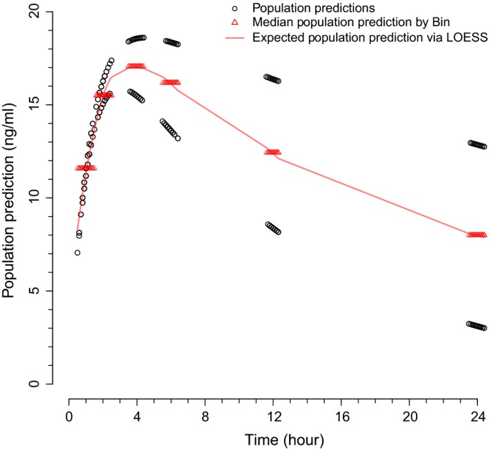
Median population predictions by bin and expected population predictions via LOESS for a hypothetical pharmacokinetic example. The approach to prediction‐corrected visual predictive checks in the current work involves normalizing the population predictions (black open circles) to the expected population predictions via LOESS (red solid line), rather than to the median of the population predictions for each bin (red open triangles).

Evaluation of VPCs via regression techniques

The proposed approach to VPCs and pcVPCs was evaluated in five scenarios. Detailed descriptions are provided below.

Hypothetical population PK

The first scenario used simulated data from a hypothetical one‐compartment PK model (ka = 0.80, CL/F = 8.0 L/h, V/F = 100 L; corresponding between‐subject variances of 0.20, 0.02, and 0.01; proportional residual variance of 0.025). A drug interaction effect, indicated by the presence or absence of a hypothetical concomitant medication, was incorporated into CL/F (fractional effect of 0.25). A total of 100 virtual subjects were simulated, with 50 subjects on the concomitant medication and 50 subjects off the concomitant medication.

Each subject received the same dose of the hypothetical drug (2 mg) and had six samples taken (1, 2, 4, 6, 12, and 24 hours postdose, with random noise added to each time point). The population PK model used for simulation was fitted to the simulated PK data. VPCs via AQR were performed for subjects on and off the concomitant medication separately and a pcVPC via LOESS and AQR was derived for all subjects. The VPCs and pcVPCs characterized the 10th, 50th, and 90th percentiles of the original and simulated PK profiles. The smoothing parameters for AQR and LOESS, λ and α, were determined by optimization based on the original (simulated) PK data. Throughout, optimization procedures for λ and α were based on previous research.10, 16, 17, 18 The VPCs and pcVPCs were generated using 500 replicates of the original (simulated) PK data. To ensure the proposed approach could yield results similar to a conventional bin approach (expected in this simplistic scenario), the VPCs and pcVPC were re‐derived by empirical bin selection, where the bins were determined based on the nominal sampling times noted above.

Warfarin population PK‐pharmacodynamics

The second scenario utilized publicly available PK‐pharmacodynamic (PD) data and NONMEM19 code for warfarin.20 Two different population PK‐PD models were fitted to the data: an effect‐compartment model and a turnover model. Corresponding VPCs via AQR were derived to evaluate and discriminate between the two models. The VPCs characterized the 10th, 50th, and 90th percentiles of the original and simulated PK‐PD profiles. The corresponding λs were determined by optimization based on the original data. The VPCs were generated using 500 replicates of the original data. For the simulated profiles simulation‐based 95% confidence intervals (CIs), were derived for each percentile.21

Phenobarbital population PK

The third scenario used example PK data and NONMEM code provided with Perl‐Speaks‐NONMEM (PsN version 4.6.0),5, 6 which is freely available. The data consisted of 59 neonates who received intravenous phenobarbital. The population PK model consisted of one compartment with a linear weight effect on CL/F. A pcVPC was derived using LOESS and AQR, which characterized the 10th, 50th, and 90th percentiles of the original and simulated profiles. The smoothing parameters α and λ were determined by optimization based on the original data. To ensure consistency with PsN, additional pcVPCs were derived using PsN's vpc command, where the autobin option was used to specify 5, 8, and 10 bins. All pcVPCs were generated using 500 replicates of the original data. For the simulated profiles, 95% CIs were derived for each percentile.

Hypothetical population PK with intensive and sparse sampling

The fourth scenario comprised simulated data from a hypothetical one‐compartment PK model with allometry on CL/F and V/F (ka = 0.80, CL/F = 8.0 L/h/70 kg, V/F = 100 L/70 kg). A total of 200 virtual subjects were included, with 100 subjects on 2 mg and 100 subjects on 4 mg of the hypothetical drug. Dosing was once daily for 8 weeks. A subset of 30 subjects had intensive sampling at 1, 4, 8, 12, and 24 hours after the first dose. All subjects had trough samples taken at days 28 and 56 (within 3 days for both time points). The pcVPCs were generated using the proposed approach. The α and λ parameters were determined by optimization based on the original data. For the simulated percentiles, 95% CIs were displayed.

Hypothetical population PK‐viral kinetics

The last scenario was a population analysis of hypothetical (simulated) PK‐viral kinetic (VK) data. The model used for simulation was based on previously published work22 (see Appendices S1 and S2 for further details). The PK‐VK profiles were simulated for 30 virtual subjects, with 7 time points per subject. The profiles included a substantial proportion of data below the lower limit of detection (LLOD; ~43% of all data). As such, these (simulated) data were analyzed in NONMEM using the structural model used for simulation (Appendices S1 and S2) and NONMEM's M3 method23 to account for censored data. A VPC via AQR was constructed to accommodate the handling of data below the LLOD in the analysis. Specifically, for the observed data, observations indicated as LLOD were imputed based on methods presented elsewhere24 (details in Appendices S1 and s2). Thus, AQR for the observed data included data above and below the LLOD, where the latter were imputed. Simulations were performed using the parameter estimates achieved via M3. The 10th, 50th, and 90th percentiles of the observed and simulated PK‐VK profiles were characterized, where the corresponding λs were determined by optimization based on the observed data. For the simulations, 95% CIs were derived for each percentile.

Additionally, the cumulative proportion of data LLOD over time was calculated for the observed and simulated data, where AQR (median only) was used to characterize the trend. The λ parameter was determined by optimization of the observed data. For the simulations, a 95% CI (for the median) was derived.

Software

The hypothetical PK and PK‐VK data were generated with the mrgsolve package in R25; analyses and simulations were performed in NONMEM19 via PsN version 3.7.6.5, 6 Analyses and simulations for the warfarin PK‐PD scenario were performed in NONMEM via Wings for NONMEM26 using previously written control streams.20 NONMEM via PsN was used for analysis and simulations for the phenobarbital scenario, where control streams were provided by PsN. For all scenarios, the VPCs and pcVPCs via LOESS and/or AQR were derived in R version 3.3.113 by applying the loess,17 loess.as,18 and rqss15 routines. The VPCs and pcVPCs via empirical bin selections were derived in R version 3.3.1 for the first hypothetical PK scenario; PsN and Xpose27 were used for the phenobarbital example. All work was performed on a laptop computer with a 64‐bit operating system, Intel Core i7‐6600U CPU (2.60 GHz 2.81 GHz) and 20 GB of random access memory.

Results

Hypothetical population PK

The VPCs and pcVPCs derived using the proposed approach were similar to those derived from empirical bin selection (Figure  2). For subjects off and on the concomitant medication, optimization for λ, which was based on the original (simulated) data, took between 0.3 and 0.5 seconds per quantile (i.e., the 10th, 50th, or 90th percentile). Application of AQR to the original data took ~0.016 seconds per quantile and performing AQR across the 500 replicates of the original data took ~30 seconds.

Figure 2.

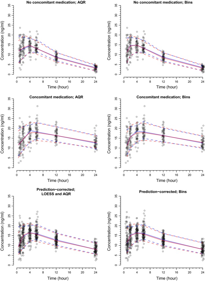
The visual predictive checks (VPCs) for the hypothetical one‐compartment population pharmacokinetic model. The left and right columns of the figure display VPCs via regression and empirical bin selection, respectively. For all plots, the blue solid line represents the observed median and the blue dashed lines represent the observed 10th and 90th percentiles. Similarly, for all plots, the red solid line represents the simulated median and the red dashed lines represent the simulated 10th and 90th percentiles. AQR, additive quantile regression.

For the pcVPC, it took ~0.1 seconds to optimize for α, between 0.4 and 0.5 seconds per quantile to optimize for λ (again based on the original data) and 0.015 seconds per quantile to apply AQR to the original data. It took ~35 seconds to apply AQR across the 500 replicates.

Warfarin population PK‐PD

The VPCs via AQR correctly highlighted the acceptable fit of the effect‐compartment model and the ideal fit of the turnover model (Figure  3). Optimization for λ, which was based on the original data, took between 0.2 and 0.5 seconds per quantile. For both models, it took ~0.016 seconds per quantile to apply AQR to the original data and ~25 seconds to perform AQR across the 500 replicates.

Figure 3.

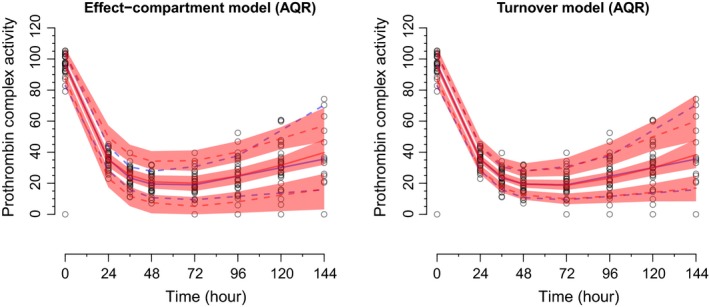
The visual predictive checks (VPCs) for the population pharmacokinetic‐pharmacodynamic models of warfarin. The left and right plots display the VPCs for the effect‐compartment and turnover models, respectively. For both plots, the blue solid line represents the observed median and the blue dashed lines represent the observed 10th and 90th percentiles. Similarly, for both plots, the red solid line represents the simulated median and the red dashed lines represent the simulated 10th and 90th percentiles. The pink shaded regions indicate 95% confidence intervals for the simulations. AQR, additive quantile regression.

Phenobarbital population PK

The pcVPCs via LOESS/AQR and empirical bin selection highlighted that on median, the model underpredicted the 10th and 50th percentiles of the data (Figure  4). However, large variation was observed for the simulated percentiles, as indicated by the 95% CIs. For the pcVPC via LOESS and AQR, it took ~0.03 seconds to optimize for α, 0.3 seconds per quantile for λ optimization, 0.016 seconds per quantile for application of AQR to the original data, and 31 seconds to run AQR across the 500 replicated data sets. The pcVPCs via empirical bins varied in appearance by the number of bins specified. In addition, for all pcVPCs via empirical bins, the last bin was very wide due to sparse sampling within the time interval of 200–400 hours. This led to these pcVPCs being truncated at ~300 hours (i.e., the midpoint of the last bin). In contrast, the pcVPC from the proposed (regression) approach spanned the entire profile.

Figure 4.

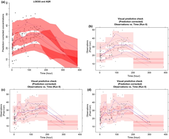
The prediction‐corrected visual predictive checks (pcVPCs) for the population pharmacokinetic model of phenobarbital. For all plots, the blue solid line represents the observed median and the blue dashed lines represent the observed 10th and 90th percentiles. Similarly, for all plots, the red solid line represents the simulated median and the red dashed lines represent the simulated 10th and 90th percentiles. The pink shaded regions indicate 95% confidence intervals for the simulations. AQR, additive quantile regression.

Hypothetical population PK with intensive and sparse sampling

For this scenario, optimization of α and λ was performed initially using all observed data (i.e., intensive and sparse combined). However, this resulted in misspecified LOESS and AQR fits for the subset of subjects with intensive sampling, because optimization was biased toward the trough/sparse samples (i.e., the majority of the data). This was rectified by performing the pcVPCs by clinic visit (first day (n = 30); day 28 (n = 200); and day 56 (n = 200)). This was achieved by writing a simple loop in R. After this modification, the resulting pcVPCs were acceptable (Figure  5). It took ~2 minutes to generate the stratified pcVPCs in Figure  5.

Figure 5.

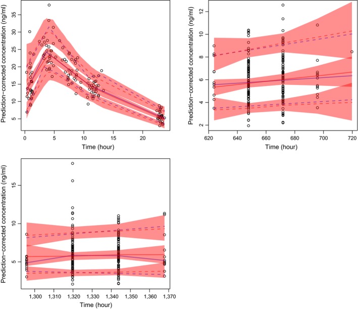
The visual predictive checks for the hypothetical population pharmacokinetic model with intensive and sparse sampling. The subset of intensive subjects is displayed in the upper left panel. The top right and bottom left panels display trough/sparse sampling for all subjects. For all plots, the blue solid line represents the observed median and the blue dashed lines represent the observed 10th and 90th percentiles. Similarly, for all plots, the red solid line represents the simulated median and the red dashed lines represent the simulated 10th and 90th percentiles. The pink shaded regions indicate 95% confidence intervals for the simulations.

Hypothetical population PK‐VK

The VPCs correctly highlighted the appropriateness of accounting for censored (i.e., LLOD) data in this scenario (Figure  6). The VPCs also (correctly) showed that the model could simulate LLOD data consistent with what was observed. For the observed data, it took ~0.4–0.6 seconds per quantile for λ optimization and 0.02–0.03 seconds per quantile to apply AQR. It took ~30 seconds to apply AQR across the 500 replicates.

Figure 6.

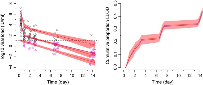
The visual predictive checks for the population pharmacokinetic‐viral kinetic scenario. For the left plot, the dashed line indicates the lower limit of detection (LLOD), the blue solid line represents the observed median, the blue dashed lines represent the observed 10th and 90th percentiles, the red solid and dashed lines indicate the corresponding simulated percentiles, the pink shaded regions indicate 95% confidence intervals (CIs) for the simulations and the circled purple crosses represent imputed data below the LLOD. For the right plot, the blue solid line represents the observed median, the red solid line represents the simulated median, and the pink shaded region indicates the 95% CI for the simulated median.

For the cumulative proportion LLOD, it took ~0.5 seconds for λ optimization and 0.02 seconds to apply AQR (median only for both). It took ~10 seconds to apply AQR across the 500 replicates (again median only).

Discussion

This work proposed the use of regression techniques to perform VPCs and pcVPCs for population pharmacometric models. This alternative approach was shown to be accurate and reliable within evaluation scenarios representative of typical application. The method utilized well‐established statistical techniques and was straightforward to implement.

A highlight of the current work was the extension of the existing, novel methodology for pcVPCs.14 This extension involved normalizing model‐derived population predictions to those expected from LOESS, rather than to the median of the population predictions for each bin. As such, this new approach to pcVPCs may offer improved accuracy in scenarios where bins are required to be wide or highly variable in width due to sparse or irregular sampling, poor design implementation, or other issues. This was shown in the phenobarbital example, where the pcVPC from the proposed approach spanned the entire PK profile in the presence of sparse/irregular sampling at late time points. This provided more information than the pcVPCs derived from bins (via autobin in PsN), which were truncated due to the sparse/irregular sampling. Moreover, the categorical nature of the bins yielded 95% PIs (via Xpose) that were discontinuous and somewhat difficult to interpret.

Another highlight of the current work was the application of the proposed method in a scenario where censored data (i.e., below the LLOD) were accounted for in the analysis (i.e., the hypothetical population PK‐VK model). The proposed methodology yielded VPCs that were accurate and easy to interpret. Furthermore, the transparency of the method, particularly with imputation of censored values (i.e., below the LLOD), offers readers the ability to reproduce the examples and adapt as necessary for future applications.

The computational expense of the proposed approach was acceptable in the evaluation scenarios. However, it is pertinent to note that computation time for the new method is relatively longer than conventional binning approaches. This is to be expected because regression techniques are more computationally demanding than computing simple percentiles within user‐defined bins. Nevertheless, computation time for the proposed approach should still be acceptable for modern personal computers. Moreover, it is important to highlight that even though binning procedures, such as autobin in PsN, offer computational efficiency, to the best of our knowledge, such procedures generate bins to ensure they have approximately equal numbers of observations and/or similar variances of the dependent variable. Hence, these kinds of procedures do not optimize directly for the shape of the pharmacometric profile, and, thus, may not necessarily produce bins that provide means for accurate characterization. Therefore, key advantages of the proposed approach are convenience (i.e., not having to determine bins) and possible improved accuracy, at the expense of some computation time. Future applications of the methodology will reveal how it performs in different scenarios.

The VPCs and pcVPCs presented in this work were derived in R13 using the loess and rqss routines. However, other statistical packages could have been used, such as Stata28 or SAS.29 In the current work, R was chosen for its accessibility and growing use within the pharmacometrics community. Moreover, implementation in R did not require advanced programming.

Despite the strengths of performing VPCs and pcVPCs via regression, the approach is not without possible limitations. For instance, it is possible that implementing LOESS or AQR may be problematic in some scenarios, such as extremely sparse sampling, poor design implementation, uninformative sampling, very small numbers of subjects, highly variable sampling across the profile, extreme residual variability, etc. If LOESS or AQR cannot be achieved (or achieved adequately) with the observed data, other approaches, such as empirical bin selection, may be required. However, in such scenarios, VPCs and/or pcVPCs via empirical bin selection may be highly sensitive to the choice of bins. The longitudinal nature of the data was not accounted for in the AQR procedure used in this work (i.e., a grouping or clustering variable, such as subject identifier, is not specified in rqss15). As such, if confidence intervals or PIs for the estimated quantiles are to be derived, appropriate empirical procedures accounting for the longitudinal nature of the data should be employed. For instance, clustered bootstrap for observed data and methodology proposed previously for simulations2 (the latter was used for the evaluation scenarios). Importantly, appropriate specification of α and λ is crucial for the accuracy of the proposed approach. Therefore, it is recommended to optimize for α and λ first when applying LOESS and AQR (respectively) to the observed data, then inspect visually to ensure the corresponding fitted values are consistent with the observed data. The importance of this step was shown in the scenario with sparse and intensive PK sampling, as visual inspection revealed that optimization had to be stratified by clinic visit to yield sensible results. Optimization can be an efficient and objective way to specify these important parameters. Moreover, more sophisticated optimization algorithms than those presented in this work may be used but may come at the expense of computation time.

Last, the authors would like to reiterate that this work is an extension of current VPC methodology, offering enhanced convenience and statistical rigor. Hence, it is not our intention to discredit previous/conventional approaches, but rather, to offer another way for performing this useful diagnostic procedure. For instance, the new approach could be used as a sensitivity check for conventional binning approaches.

Conclusions

This work provides support for using regression techniques, namely LOESS and AQR, to perform VPCs and pcVPCs for population pharmacometric models. This alternative approach negates the need for empirical bin selection.

Funding

No funding was received for this work.

Conflict of Interest

The authors declared no competing interests for this work.

Author Contributions 

K.M.J. and K.P. wrote the manuscript. K.M.J., C.M.J.K., and K.P. designed the research. K.M.J., K.P., K.N., and C.M.J.K. performed the research.

Supporting information

References

- 1. Karlsson, M.O. & Holford, N. Abstracts of the Annual Meeting of the Population Approach Group in Europe. A tutorial on visual predictive checks. Abstract 1434. < http://www.page-meeting.org/?abstract=1434 > (2008).
- 2. Karlsson, M.O. & Holford, N. Model evaluation: visual predictive checks. < http://www.page-meeting.org/pdf_assets/8694-Karlsson_Holford_VPC_Tutorial_hires.pdf > (2008).
- 3. Lavielle, M. & Bleakley, K. Automatic data binning for improved visual diagnosis of pharmacometric models. J. Pharmacokinet. Pharmacodyn. 38, 861–871 (2011). [DOI] [PubMed] [Google Scholar]
- 4. Sonehag, C. , Olofsson, N. & Simander, R. Automatic binning in visual predictive checks. < http://www.it.uu.se/edu/course/homepage/projektTDB/ht11/project4/Report_ht11_04.pdf > (2012).
- 5. Lindbom, L. , Ribbing, J. & Jonsson, E.N. Perl‐speaks‐NONMEM (PsN) – a Perl module for NONMEM related programming. Comput. Methods Programs Biomed. 75, 85–94 (2004). [DOI] [PubMed] [Google Scholar]
- 6. Lindbom, L. , Pihlgren, P. & Jonsson, E.N. PsN‐Toolkit – a collection of computer intensive statistical methods for non‐linear mixed effect modeling using NONMEM. Comput. Methods Programs Biomed. 79, 241–257 (2004). [DOI] [PubMed] [Google Scholar]
- 7. Koenker, R. Quantile Regression (Cambridge University Press, London, UK, 2005). [Google Scholar]
- 8. Cleveland, W.S. Robust locally weighted regression and smoothing scatterplots. J. Am. Stat. Assoc. 74, 829–836 (1979). [Google Scholar]
- 9. Koenker, R. & Ng, P. A Frisch‐Newton algorithm for sparse quantile regression. < http://www.econ.uiuc.edu/~roger/research/sparse/fn3.pdf > (2005).
- 10. Koenker, R. Additive quantile regression: model selection and confidence bandaids. Braz. J. Probab. Stat. 25, 239–262 (2011). [Google Scholar]
- 11. Koenker, R. , Ng, P. & Portnoy, S. Quantile smoothing splines. Biometika 81, 673–680 (1994). [Google Scholar]
- 12. Koenker, R. & Mizera, I. Penalized triograms: total variation regularization for bivariate smoothing. J. R. Stat. Soc. Series B Stat. Methodol. 81, 145–163 (2004). [Google Scholar]
- 13. R Core Team . R: A Language and Environment for Statistical Computing (R Foundation for Statistical Computing, Vienna, Austria, 2016). < https://www.R-project.org/ >. [Google Scholar]
- 14. Bergstrand, M. , Hooker, A.C. , Wallin, J.E. & Karlsson, M.O. Prediction‐corrected visual predictive checks for diagnosing nonlinear mixed‐effects models. AAPS J 13, 143–151 (2011). [DOI] [PMC free article] [PubMed] [Google Scholar]
- 15. Koenker, R. Quantreg: Quantile Regression, version 4.45. http://cran.r-project.org/package=quantreg (2010). [Google Scholar]
- 16. Hurvich, C.M. , Simonoff, J.S. & Tsai, C.‐L. Smoothing parameter selection in nonparametric regression using an improved Akaike information criterion. J. R. Stat. Soc. Series B Stat. Methodol. 60, 271–293 (1998). [Google Scholar]
- 17. LOESS hyperparameters without tears. < http://www.wellformedness.com/blog/category/stats/r/ > (2013).
- 18. Wang, X.‐F. fANCOVA: Nonparametric Analysis of Covariance. R package version 0.5‐1. < https://CRAN.R-project.org/package=fANCOVA > (2010). [Google Scholar]
- 19. Beal, S. , Sheiner, L.B. , Boeckmann, A.J. & Bauer, R.J. NONMEM User's Guides (Icon Development Solutions, Ellicott City, MD, 1989. –2009). [Google Scholar]
- 20. Holford, N. PKPD workshop. < http://holford.fmhs.auckland.ac.nz/docs/pkpd-workshop-nonmem7.pdf >.
- 21. Nguyen, T.H. et al Model evaluation of continuous data pharmacometric models: metrics and graphics. CPT Pharmacometrics Syst. Pharmacol. 6, 87–109 (2017). [DOI] [PMC free article] [PubMed] [Google Scholar]
- 22. Laouénan, C. , Guedj, J. & Mentré, F. Clinical trial simulation to evaluate power to compare the antiviral effectiveness of two hepatitis C protease inhibitors using nonlinear mixed effect models: a viral kinetic approach. BMC Med. Res. Methodol. 13, 60 (2013). [DOI] [PMC free article] [PubMed] [Google Scholar]
- 23. Bergstrand, M. & Karlsson, M.O. Handling data below the limit of quantification in mixed effect models. AAPS J 11, 371–380 (2009). [DOI] [PMC free article] [PubMed] [Google Scholar]
- 24. Nguyen, T.H. , Comets, E. & Mentré, F. Extension of NPDE for evaluation of nonlinear mixed effect models in presence of data below the quantification limit with applications to HIV dynamic model. J. Pharmacokinet. Pharmacodyn. 39, 499–518 (2012). [DOI] [PubMed] [Google Scholar]
- 25. Baron, K.T. , Hindmarsh, A.C. , Petzold, L.R. , Gillespie, B. & Margossian, C. Simulation from ODE‐based population PK/PD and systems pharmacology models in R using mrgsolve. < https://metrumrg.com/event/simulation-ode-based-population-pk-pd-systems-pharmacology-models-r-using-mrgsolve/ >.
- 26. Holford, N. Wings for NONMEM. < http://wfn.sourceforge.net/ > (2017).
- 27. Harling, K. , Ueckert, S. , Hooker, A.C. , Jonsson, E.N. & Karlsson, M.O. Xpose and Perl speaks NONMEM (PsN). Abstract of the Annual Meeting of the Population Approach Group in Europe. < http://www.page-meeting.org/?abstract=1842 > (2010).
- 28. StataCorp. Stata Statistical Software: Release 14 (StataCorp LP, College Station, TX, 2015). [Google Scholar]
- 29. SAS Institute Inc. Base SAS 9.3 Procedures Guide (SAS Institute Inc, Cary, NC, 2011). [Google Scholar]
Associated Data
This section collects any data citations, data availability statements, or supplementary materials included in this article.
Supplementary Materials