Kilobase Pair Chromatin Fiber Contacts Promoted by Living-System-Like DNA Linker Length Distributions and Nucleosome Depletion

Abstract

Nucleosome placement, or DNA linker length patterns, are believed to yield specific spatial features in chromatin fibers, but details are unknown. Here we examine by mesoscale modeling how kilobase (kb) range contacts and fiber looping depend on linker lengths ranging from 18–45 bp, with values modeled after living systems, including Nucleosome Free Regions (NFRs) and gene encoding segments. We also compare artificial constructs with alternating versus randomly distributed linker lengths in the range of 18–72 bp. We show that non-uniform distributions with NFRs enhance flexibility and encourage kb-range contacts. NFRs between neighboring gene segments diminish short-range contacts between flanking nucleosomes, while enhancing kb range contacts via hierarchical looping. We also demonstrate that variances in linker lengths enhance kb range contacts. In particular, moderate sized variations in fiber linker lengths (∼27 bp) encourage long range contacts in randomly distributed linker length fibers. Our work underscores the importance of linker length patterns in biological regulation.

Contacts formed by kb-range chromatin folding are crucial to gene activity. Because we find that special linker length distributions in living systems promote kb contacts, these patterns together with bound proteins, are crucial to regulation of gene activity.

Graphic Abstract

Introduction

The structure of chromatin, the nucleic acid/protein complex that packages DNA in eukaryotic nuclei, is of fundamental importance to the regulation of life’s basic processes. Yet, the chromatin architecture is not well understood on many spatial scales, from fibers to chromosomes. At the finest level of organization, ∼147 base pairs (bp) of double stranded DNA wraps ∼1.75 times around a core of 8 histone proteins, two copies each of the H2A, H2B, H3 and H4 proteins, forming the nucleosome core particle.¹ When nucleosomes are spaced along DNA, they form a ‘beads-on-a-string’ structure, named after its appearance under an electron microscope.² This structure then undergoes further folding, constituting chromatin fibers.³ Chromatin fibers, which span thousands of base pairs (kb), further organize into discrete compartments termed Topologically Associating Domains (TADs) that can span millions of base pairs (Mb).⁴ Chromosomes contain hundreds to thousands of TADs.⁴ While many higher-order chromatin fiber structures have been proposed,^5,6 investigating the specific structure of living chromatin fibers, and the dependence of this structure on internal factors, such as the DNA linker length and post-translational marks of histone tails, remains an active area of research.^6–8

Experimentally, chromatin fibers can be characterized using a variety of techniques. For example, X-ray crystallography and cryo-EM techniques have been used to image the nu-cleosome core particle^1,9 as well as short fibers.¹⁰ Larger fibers cannot be directly imaged, but have been examined by various chromatin cross-linking techniques that generate internucleosomal contact probabilities as a function of nucleosome separation.¹¹ Conformation capture techniques (such as Hi-C) report nucleosome contacts spanning kilo-base pairs (kb) to mega-base pairs (Mb).¹² Specialized Hi-C variants, such as Micro-C, report these contacts at nucleosome resolution, but currently are only available in yeast.¹³ The Cryo-EM Assisted Nucleosome Interaction Capture technique (EMANIC) reports nucleosome resolution contact frequencies in human cell lines, but cannot currently distinguish between various genes, as it does not incorporate sequence data.^11,14

To interpret the range of information such assays provide, it has become customary to discuss chromatin fibers in terms of internucleosome interaction probability, i.e., the probability that a given nucleosome i will be in contact with some other nucleosome i ± k nucleosomes distant on the fiber. Dominance of near-neighbor nucleosome contacts (i.e., a majority of i±1 internucleosome contact probability) is associated with bent linker DNA, or a solenoid-type folding motif; next-neighbor dominance (i.e., a majority of i ± 2 internucleosome contact probability) is associated with zigzag folding and straight linker DNAs. Although recent studies indicate i±2 contacts dominate chromatin contact probability profiles derived from in vivo systems both for human^14,64 and yeast,¹⁵ these studies also show i ± 1 contacts and increased kb range contacts. This duality may be indicative of fluid, heteromorphic, selfassociating fibers as opposed to stiff 30 nm fibers reported by in vitro assays.¹⁶ Additionally, recent studies have not identified 30 nm signatures in living systems. Instead, forms with 10 nm diameters are suggested, also associated with the unfolded ‘beads-on-a-string’ motif.¹⁸ Thus, the common emerging view is of chromatin fibers organized as fluid entities, folded into dynamic loops of various size, while loosely exhibiting local zigzag folding, with modest content of bent DNA linkers.¹⁷

This fluid description is crucial to interpreting gene regulation, long viewed as a stochastically driven time-dependent process sensitive to nucleosome positioning, DNA sequence, and many factors in the cell nuclear environment.¹⁹ The amount of DNA linking successive nucleosomes, in particular, is known to vary across cell content, species, and cycle.⁶ This linker length is often measured by the Nucleosome Repeat Length or NRL (NRL = DNA linker length + 147 bp), historically measured by micrococcal nuclease chromatin digestion, wherein linker DNA is cut by the enzyme and DNA protected by a nucleosome remains intact. The length of resulting fragments are then measured, and the average length is considered the measured NRL.²⁰ In general, short DNA linker lengths are associated with high levels of gene expression²² that exhibit 10n +5 periodicity,²¹ although species specific differences near transcription start sites have recently been demonstrated.²¹

Recent advances in nucleosome positioning assays, however, bring more detail to this topic. Incorporation of engineered sulfur tagged histones, in conjunction with a copper chelating agent, now make possible base pair resolution measurements of nucleosome positions. These are now available for 3 different species, including the budding yeast, S. Cerevesiae,²³ fission yeast, S. Pombe,²⁴ and mouse Embryonic Stem Cells (mESC),²¹ whose genomes show specific distributions of linker lengths across the genome. Yeast chromatin, in aggregate, exhibits a distribution of 10n+5 DNA linker lengths, for n = 0,1,2,3,4, and 5. S. Pombe chromatin exhibits a median DNA linker length of 5 bp (NRL of 152 bp), with small amounts of 15 bp (∼ 25%) and 25 bp (∼10%) linkers (NRL of 162 bp and 172 bp), respectively. S. Cerevesiae chromatin displays a wider distribution of linker lengths spanning from 5 to 45 bp (NRLs of 152 to 192 bp), with a strong peak at 15 bp.²³ S. Cerevesiae chromatin linker lengths are composed of roughly 30% 5 bp, 35% 15 bp, 20% 25 bp and 10% 35 bp. Genome-wide mouse cells similarly show a 10n+5 linker length preference, but n = 1,2,3,4,...10, with a median linker length at 35 bp and 45 bp (NRL of 182 and 192 bp).²¹ It is unknown, however, what effects these distributions have on overall fiber structure, or whether the same distributions extend to other species or differentiation states, including human cell lines, which show an average linker length of 55 bp (NRL of 201 bp).²⁵ Furthermore, studies suggest that active genes tend to show a 10n+5 periodicity and inactive genes show a 10n bp periodicity.²¹ It was later suggested by modeling that this trend is related to the periodicity of the DNA double helix, where DNA topology plays structural roles in the stability of the fiber.^26,27

These recently identified patterns in nucleosome positions suggest a new level of chromatin structural complexity that relates structure to gene expression. Moreover, kb range chromatin contacts that are crucial for genetic regulation may depend sensitively on these patterns.²⁸ In genome-wide yeast contact profiles, for example, domains of increased contact density are noted in the short to medium contact range (1–10 nucleosomes, or sub-kb) named Chromosomally Interacting Domains (CIDs), analogous to Topologically Associating Domains (TADs) in human chromatin.^13,15 CIDs are separated by nucleosome depletions and boundary elements such as CTCF proteins.⁵ The healthy maintenance of these boundaries in humans have recently been linked to the activation of proto-oncogenes²⁹ and problems in developing embryos in mice.³⁰ Each CID or TAD spans 1–4 gene encoding regions.³¹ Each gene encoding region spans 2–6 nucleosomes on average, and is flanked by Nucleosome Free Regions (NFRs) at both the 5^′ and 3^′ ends of the region.²³ Nucleosome positioning assays report that the first 2–3 nucleosomes downstream of the 5^′ NFR are strongly positioned, i.e., are tightly spaced at regular intervals (with an average linker length of ∼15 bp), whereas nu-cleosomes near the 3^′ end of the gene encoding region are positioned more stochastically.^23,31

The specific looping dynamics of these chromosomal domains and their respective gene encoding segments, however, in any specific organism, are difficult to deduce because the data reported are generally averaged across large cell populations.³² Although still preliminary, single molecule chromatin conformation capture assays, in conjunction with polymer modeling, suggest that no single loop or fold represents the contacts within a TAD; instead, they are likely the average representation of a dynamically extruding loop that is being guided through a small pore in the condensin protein,³³ helping to maintain a variety of contacts across the domain. Recent extension of these results to TADs rich in promoters shows that there may be even more preferential binding across promoters and enhancers within the TAD, possibly mediated by extrusion-like mechanisms.²⁸ Loop extrusion is likely guided by a combination of condensin proteins and DNA binding proteins, which act as boundary elements (such as CTCF proteins).^33,34

A variety of computational methods have been successfully applied to investigate chromatin; see recent reviews.^17,35,36 While all-atom models can treat proteins and nucleosomes,³⁷ they are prohibitively expensive for simulating larger systems due to the large number of atoms in the solute and solvent. Coarse-grained models which use individual amino or nucleic acid residues as the basic subunit of modeling, can treat slightly larger systems, for example for investigating the dynamics of nucleosomal wrapping and unwrapping events,³⁸ but are still limited to small numbers of nucleosomes due to large system sizes. Polymer models, which treat kb-size fiber fragments as the basic subunit of modeling, can treat chromosomes and Mb range contacts, but lack the necessary resolution to explore specific effects of DNA linker length on fiber structure.³⁹ Mesoscale chromatin models, however, which treat each nucleosome as the basic subunit of modeling, can generate nucleosome-contact maps spanning kb range contacts to study elements of the structures discussed above.³⁵ Such structural characterization is particularly complementary to ultrastructural experiments, like EMANIC,¹⁴ which captures and visualizes internucleosome contacts on the kb level via formaldehyde fixation and electron-microscopy imaging. Additional ultrastructural data come from MicroC, which captures genome-wide internucleosome contacts with nucleosome resolution,¹⁵ and super-resolution imaging techniques like STORM, which, in association with in vivo fluorescence labeling, can determine the surface area and volume of specific genes in various epigenetic states.⁴⁰

Here we investigate the role of nucleosome positioning, or variations in DNA linker length, on chromatin fiber interactions in the kb range. Although there has been much modeling work on fibers with uniform DNA linker lengths in the kb range (e.g.,^27,41) fibers with non- uniform DNA linker lengths have only recently been considered^42,43 but not with values mimicking living systems like those found by recent genome-wide nucleosome positioning assays.^23,24 Here we present a systematic investigation of representative DNA linker length distributions, with and without explicitly modeled NFRs, and report resulting persistence lengths and internucleosome contact probability profiles, along with a self-association measure we have developed for quantifying the nature of non-local contacts within a large folded fiber. We find that, unlike reference constructs, non-uniform linker length distributions with NFRs lead to enhanced long-range contacts via looping in the kb range. This suggests that this local variable profoundly affects global chromatin architecture and hence gene regulation.

Computational Methods

Mesoscale Model.

Our mesoscale chromatin model consists of four bead/particle types: linker DNA, nucleosome core particle psuedo-charges, flexible histone tails, and linker histone (LH). A full discussion is given in Ref.⁴⁴ In brief, the linker DNA is treated as a modified worm-like chain,^41,45 with parameters developed using Stigter’s procedure.⁴⁶ Each linker DNA bead represents ∼ 9 base pairs.⁴¹ The nucleosome core particles are represented as rigid electrostatic objects; the coarse-grained shape and surface charges are derived from our Discrete Surface Charge Optimization (DiSCO) algorithm,⁴⁷ which approximates the electric field of the atomistic nucleosome (PDB 1KX5) by placing pseudo-charges along the surface of the complex as a function of monovalent salt values.^9,48 The flexible histone tails are coarse grained so that 50 histone tail beads represent the 8 histone tails (two copies each of H2A, H2B, H3, and H4). Each histone bead represents about 5 amino acid residues. Histone tail bend, stretch, excluded volume, and partial charges were derived from all-atom Brownian dynamics simulations.⁴⁹

LH beads are coarse-grained based on a crystal structure of the H1.4 globular head and homology models of the C-terminal domain, so that 6 beads represent the globular head, and 22 beads represent the C-terminal domain, modeled after the rat H1.4 linker histone.⁵⁰

Energy terms include bend, stretch, and twist terms for linker DNA and histone tail beads, a Debye-Hückel electrostatic interaction term for all charged segments, and excluded volume terms represented by a modified Lennard-Jones potential for all beads.⁴⁴ Coordinates are computed and propagated via a local coordinate frame: Euler vectors are used to track the pitch, roll, and twist of each nucleosome, and then to calculate the corresponding linker DNA and tail coordinates, as described in detail previously.⁴¹ Specific parameters for energy terms and simulation conditions are given in Table 1.

Table 1:

Model Parameters

Parameter	Value
DNA Persistence Length	50 nm
DNA Stretching rigidity, h	6.4 kcal/mol/n2
DNA Bending Rigidity, g	5.8 kcal/mol
DNA Twisting Rigidity, s	14.3 kcal/mol
DNA Equilibrium Twist Value, φ0	.033 ± .209 rad (0 ± 12 ◦)
van der Waals radius (DNA-DNA), σl−l	3.6 nm
van der Waals radius (DNA-Core), σl−c	2.4 nm
van der Waals radius (DNA-Tail), σl−t	2.7 nm
van der Waals radius (DNA-LH, Globular head), σlLHg	3.4 nm
van der Waals radius (DNA-LH, C-term), σl−LHc	3.6 nm
van der Waals radius (Core-Tail), σc−t	1.8 nm
van der Waals radius (Core-LH, Globular head), σc−LHg	2.2 nm
van der Waals radius (Core-LH, C-term), σc−LHc	3.4 nm
van der Waals radius (Tail-LH, Globular head), σt−LHg	1.6 nm
van der Waals radius (Tail-LH, C-term), σt−LHc	2.7 nm
van der Waals radius (LH-LH, Globular head), σLHg−LHg	1.5 nm
van der Waals radius (LH-LH, C-term), σLHc−LHc	1.8 nm
Electrostatic Long Range Cutoff	7 nm
Lennard-Jones Long Range Cutoff	4 nm
Temperature, T	293 K
Salt Concentration (NaCl)	150 mM

Sampling Methods.

Four types of Monte Carlo (MC) moves are implemented for local and global sampling, namely a global ‘pivot’ move, a configurationally biased ‘regrow’ routine for histone tails,⁵¹ and local translation and rotation moves. The global ‘pivot’ move consists of randomly choosing one residue along the fiber and a random axis passing through the chosen component.⁴¹ The shorter half of the bisected oligonucleosome chain is then rotated around the randomly chosen axis, and the resulting configuration is subject to standard MC metropolis acceptance.⁵² In the configurationally biased regrow routine, a tail chosen at random is ‘regrown’, bead by bead, starting with the bead closest to the core, according to the Rosenbluth method.⁵³ This process is then repeated 10–12 times, and the tail configuration with lowest resulting energy is subject to Metropolis acceptance/rejection criteria. All DNA and linker histone beads are also sampled by translation and rotation moves, where the chosen bead is either translated or rotated by a random distance or along a chosen axis. All moves are then subject to standard Metropolis acceptance/rejection criteria.⁵²

Starting Configurations, Simulation Parameters, and Ensemble Generation.

All fiber systems consist of 100 nucleosomes, corresponding roughly to 17.4 kb fragments (with an average NRL of 174 bp). Starting coordinates are designed as idealized 2-start zigzag conformations with a z-rise of 3 nm and an entry-exit angle of 43.15°, as detailed previously.⁴¹ Sample starting conformations are given in Fig. S9 in supporting information. We simulated 6 fiber types with varying distributions of linker lengths, as shown in Table 2. Uniform linker length fibers contain a single value of either 18 bp or 27 bp (due to the limitations of our coarse-grained linker DNA bead representation). Life-like distributions of linker lengths are mimicked as 70% 18 bp, 20% 27 bp and 10% 36 bp similar to the form found by Brogaard et al.,²³ where we represent all ≤15 bp linker lengths with 2 beads (∼18 bp linker length) due to the resolution of coarse-grained linker beads.⁴¹ Life-like with NFRs fibers are modeled as life-like fibers above with frequent short or long NFRs. Specifically, short and long NFRs, modeled as 72 bp and 162 bp, respectively, are placed as a function of genomic positions to mimic the NFR placement in a 20 kb yeast segment following Chromosome 9 (∼260,000280,000 bp) given in Fig. 5c of reference.¹⁵ Placement details are illustrated in Table 2, where NFRs are bracketed in bold (starting conformations are also shown in supporting information Fig. S9). Gene encoding-like fibers contain similar percent composition of linker lengths as life-like fibers, but short linkers are localized near the 5^′ NFR, and linker lengths near the 3^′ NFR are distributed randomly, as observed in yeast and human cells.^23,25 For simplicity we assume that all gene orientations are the same with respect to the 3’ and 5’ ends of chromatin (see Table 2), but various orientations will be tested in the future. We also consider fibers with mixed linker lengths x,y in either randomly distributed (i.e., 50% x, 50% y) or alternating (i.e., x,y,x,y,x,y....) fashion, as given in a matrix in later figures. Specifically, the series of systems is composed of two linker lengths in the following pairs: 18/27; 18/54; 18/72; 27/36; 27/45; 36/45; 36/54; 36/63; 36/72; 45/54; 45/63; 45/72; 54/63; and 63/72 bp. Thus, the difference in linker length (ΔLL) for these 14 systems ranges from 9 to 45 bp. All linker length values used in this study and their designations are given in Table 2, except for alternating or random pairs. References to previous mesoscale modeling studies are given in the last column where possible, except for life-like, life-like with NFRs, and gene encoding-like fibers, where the reference is provided for experimental data used to model linker length or NFR content. To examine the effect of linker histone on gene-rich chromatin, we also consider gene encoding-like fibers with 1LH per 2 nucleosomes (gene encoding-like with $\frac{1}{2}LH$ ) and gene encoding-like with 1LH per nucleosome (gene encoding-like with +LH) with the above linker lengths and NFR composition as gene encoding-like fibers. Other systems do not include linker histones. All systems were run for 60–120 million steps. Energies and local/global geometric parameters were carefully monitored to ensure convergence. Error bars are derived from the variance across the last 10 million MC steps for each run. All systems were replicated in ensembles of 3–10 members, where residual twist values were adjusted by −12, 0, or +12° and run for additional steps to mimic natural variations in residual DNA twist.⁵⁴

Table 2:

Systems and linker lengths modeled. Unless otherwise stated, no linker histones are included. NFRs are denoted in brackets. For exact values of linker length pairs analyzed in systems 8 and 9, see figures.

	Designation	Composition Linker Length (bp)	Linker Length Sequence (bp)	Ref
1	Uniform	100% 18 (NRL = 165)	Uniform (18,18,18,18,18,18,18,18,18,18,...)	41
2	Uniform	100 % 27 (NRL = 174)	Uniform (27,27,27,27,27,27,27,27,27,27,...)	41
3	Life-like	70% 18, 20% 27, 10% 36	27 36 18 27 18 27 27 18 27 36 18 18 18 18 36 18 18 18 36 27 18 18 18 36 36 36 27 18 18 18 36 18 18 18 27 27 36 18 27 27 27 36 18 27 18 18 36 18 27 18 27 36 18 18 36 36 27 27 27 36 18 27 18 27 18 18 27 18 27 36 18 27 18 18 18 27 18 36 27 18 18 27 27 27 27 18 27 36 36 27 18 18 27 36 18 18 27 18 27 27	23
4	Life-like with NFRs Short NFRs: [72 bp] Long NFRs: [162 bp]	70% 18, 20% 27, 10% 36	[162] 36 18 27 18 27 27 18 [72] 36 18 18 18 18 36 18 18 [72] 36 27 18 18 18 36 [72] 36 27 18 18 [72] 36 18 18 18 27 27 36 [72] 27 27 27 36 18 27 [162] 18 36 18 27 18 27 36 18 18 36 36 27 [72] 27 [162] 18 27 18 27 18 18 27 18 27 36 18 27 [72] 18 18 27 18 36 27 18 18 27 27 27 27 18 27 36 36 27 18 18 27 36 18 [162] 27 18 27 27	15,23
5	Gene encoding-like Short NFRs: [72 bp] Long NFRs: [162 bp]	70% 18, 20% 27, 10% 36 with short linkers at the 5′ end	5′ [162] 18 18 18 18 18 27 36 [72] 18 18 18 27 18 36 27 27 [72] 18 18 18 36 18 27 [72] 18 18 18 27 [72] 18 18 18 18 18 27 36 [72] 18 18 36 27 18 27 [162] 18 18 18 27 18 36 27 18 27 18 27 36 [72] 18 [162] 18 18 18 27 18 18 18 18 27 36 18 27 [72] 18 18 18 18 18 27 18 18 27 18 36 27 18 18 36 36 18 18 18 27 36 18 [162] 18 18 18 18 3′	15,23
6	Gene encoding-like $\frac{1}{2}\text{LH}$	70% 18, 20% 27, 10% 36	″	15,23
7	Gene encoding-like +LH	70% 18, 20% 27, 10% 36	″	15,23
8	Random (7 pairs of linker lengths)	50% x (18–71), 50% y (18–71)	Random (x,y,y,x,x,y,y,x,y,x,y...)
9	Alternating (7 pairs of linker lengths)	50% x (18–71), 50% y (18–71)	Alternating (x,y,x,y,x,y,x,y,x,y...)	42

Figure 5:

Matrix of structures (lower triangle) and contact maps (upper triangle) for various combinations of NRLs alternating in sequence along the 100 core fiber. While general characteristics are shared with randomly distributed NRL sequences, subtle differences in contact types are observed, such as in the 27/45 bp systems, where long-range contacts are significantly higher than in the randomly distributed case. Additionally, hairpins form spontaneously in the 36/45 bp and 45/54 bp case which are not seen in the randomly distributed case.

All ensembles are composed of 1,000 frames (i.e., conformations) taken from the last 10 million steps of simulation trajectories. Each simulation represents an independent trajectory started from a different initial random number generator seed. Averages and standard deviations are calculated across the entire ensemble. Ensembles for systems with uniform NRLs and linker histones were composed of frames taken from 3 independent simulations, whereas all other ensembles are composed of frames taken from 10 independent simulations. The relatively large standard deviations for computed persistence lengths reflect the fluid nature of chromatin fibers, which undergo variations at thermal equilibrium. These values also reflect averaging over long simulation segments in each trajectory and over different trajectories for each condition.

Data Analysis and Computation.

We compute the fiber axis as a 3D parametric curve $r^{ax}(s)=\left(r_1^{ax}(s),r_2^{ax}(s),r_3^{ax}(s)\right)$ where each component of $r_j^{ax}$, namely j = 1,2,3, refers to the x,y, and z parametric curve components respectively. We fit the fiber axis into polynomials of the form:

$$r_j^{ax}(s)\approx P_j(i)=p_1^n(s)+p_2^{n-1}(s)\dots +p(s),$$ (1)

where the degree of the polynomial is chosen so that it fits the fiber axis by a standard least squares fitting procedure, using the MATLAB ‘polyfit’ routine. These polynomials are then used to compute the fiber axis length, compaction ratios, and persistence lengths by integrating along the fiber axis contour function $r_j^{ax}(s)$. Specifically, the persistence length is calculated by fitting an exponential to the angle defined by two unit vectors of the fiber axis parametric curve u(s) = δr^ax(s)/δs, namely the tangent vector u(s) at the initial position, and that vector position u(s^′):

$$\langle u(s)\cdot u\left(s^{\prime }\right)\rangle =\exp \left(-\left|s-s^{\prime }\right|/L_p\right),$$ (2)

where brackets indicate a mean over positions spanning the length of the fiber, and the decay length of the exponential, or the persistence length, L_p, is a measure of internal bending flexibility.⁵⁵ Thus, polymers with a short persistence length have a high occurrence of folding, whereas long persistence lengths indicate a stiff fiber with low folding propensity.

Internucleosome contact matrices are calculated by considering a “contact” (unit value) when for each fiber snapshot the elements (tail, core or linker DNA) are within the sum of the van der Waals radius (∼2 nm). These contacts are counted every 10,000 snapshots for the last 10 M snapshots of the trajectory, and normalized across all frames, as discussed in reference.¹⁴

We also define a self-association measure S_W(k), which varies from 0 to 1, and describes the density of each contact type. In other words, if S_W(1) = .5, then 50% of the nonzero off-diagonal interactions come from next-neighbor (i ± 1) internucleosome interactions. We calculate it from the contact matrix of internucleosome interactions I^′ as:

$$S_W(k)=\frac{{\displaystyle {\sum }_{i=1}^{N_C}{I}^{\prime }}(i,i\pm k)}{2{\displaystyle {\sum }_{i\ne j}{I}^{\prime }}(i,j)},$$ (3)

where S_W(1) refers to solenoid, S_W(2) to zigzag, S_W(3)+ S_W(4) to local, S_W(5)+ S_W(6) to medium, and S_W(≥ 7) to far-range contacts (where S_W(≥ 7) refers to the sum of all contacts counted for k =7,8,9,...N_C). N_C refers to the number of nucleosome cores in the system, or 100 for fibers in the present study.

All MC simulations and fiber analysis calculations were performed on the NYU High performance computing cluster, a mixed architecture platform consisting of 230 Dell Intel Nehalem nodes (2,528 cores) and 79 SUN AMD Barcelona nodes (1,264 cores).

Results

Life-like linker length distributions with NFRs decrease persistence length.

Fig. 1 shows the computed persistence length for each fiber type considered (see Table 2). For fibers with uniform linker lengths, higher average linker length is associated with increased fiber fluidity, in agreement with previous modeling results^27,41 and experimental imaging.⁵⁶ Life-like (linker lengths of 70% 18 bp, 20% 27 bp, 10% 36 bp) have a persistence length that is similar to uniform 18 bp linker length fibers, whereas NFR content decreases persistence length by as much as 20 nm. Persistence length values for these fibers are slightly shorter than those reported by older mesoscale models of chromatin,⁵⁷ although they are within a range typically reported by recent experimental studies and more recent mesoscale models: reported values computed from mesoscale models range from ∼50–280 nm based on two-angle models of uniform linker lengths at various levels of linker histone density,³⁵ and 20–75 nm for constrained chromatin loops of various size.⁴⁴ Older experimental measurements of persistence length range from ∼100–300 nm for various organisms,⁵⁸ but Sanborn et. al recently reported a measured persistence length of ∼2 kb for human cell lines via cyclization assays.³⁴ A 2 kb fragment of human chromatin corresponds to roughly 10 nucleosomes, which corresponds to an average of about ∼30–70 nm persistence length in Cartesian distance according to our models in this and previous studies, as measured by axis fitting to polynomials and associated compaction ratios (see Methods).^14,41

Figure 1:

Persistence length for systems with uniform linker length = 18 bp, uniform linker length = 27 bp, life-like, life-like with NFRs, and gene encoding-like fibers. Persistence length is calculated according to Eq. 2. A short persistence length is associated with a more flexible fiber. NFRs decrease the persistence length by ∼20 nm. Gene-encoding like fibers show slightly increased persistence length as compared to randomly distributed life-like fibers with NFRs, indicating that localizing short linkers near the 5^′ NFR stabilizes the fiber slightly. Error bars depict standard deviations, which are computed across 1,000 conformations taken from the last 10 millions steps of several independent trajectories (See Methods for details).

Life-like, life-like with NFRs, and gene encoding-like linker length systems enhance kb range contacts, while NFRs limit local contacts.

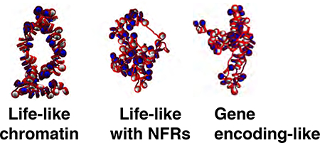
Fig. 2 shows contact matrices for these systems, with representative structures drawn for each matrix of uniform linker length = 18 bp, uniform linker length = 27 bp, life-like, life-like with NFRs, and gene encoding-like fibers. Uniform linker length fibers show limited self-association and largely lack kb range contacts. Though the fibers with uniform linker lengths of 27 bp show some kb range contacts, these are still small relative to all life-like linker length based systems. Lifelike fibers, with and without NFRs, show significant kb range contacts due to hierarchical looping, defined as a stacking network of loops in space due to close association of zigzag fiber segments. Hierarchical loops were observed by modeling and EMANIC data and proposed as a model for metaphase chromatin.¹⁴ Hierarchical loops, or lateral compaction of closely associating zigzag fibers followed by further folding in space, can be identified in contact maps as regions parallel to the main diagonal. This is in contrast to simple hairpin type loops, which correspond to regions perpendicular to the main diagonal (See Fig. 2, bottom).

Figure 2:

Contact maps and contact probability profiles for uniform linker length = 18 bp, uniform linker length = 27 bp, life-like, life-like with NFRs, and gene encodinglike fibers. Contact maps are determined by counting distances between any two fiber constituents (tail, core, or linker DNA bead) that are less than 2 nm. The 1D contact profiles are shown in the top right, indicating that long-range contacts (i± ≥ 7) are absent for short uniform linker length fibers but present for other systems. Gene-encoding like fibers show the least amount of long-range contacts. Contact matrices indicate that NFRs decrease local contacts along the diagonal, and gene-encoding like linker length distributions slightly decrease long-range (i± ≥ 7) contacts.

Notably, systems with NFRs lack local and medium-range (i ± 1,2,3) contacts near each NFR, indicative of inter-segment separation within the fiber arising from stiff doublestranded DNA in the nucleosome depleted region. Thus, while nucleosome depletion increases the overall flexibility of chromatin fibers and promotes hierarchical looping and kb range contacts (See Fig.1), it also divides neighboring gene-encoding segments. Gene encodinglike fibers show similar segmentation patterns near NFRs and hierarchical looping, but less kb range contacts, compared to life-like fibers. This is further demonstrated in the upper right of Fig. 2, where contact probability profiles are shown for uniform linker length (26 bp), life-like, life-like with NFRs and gene encoding-like fibers. The 26 bp uniform linker length fibers show zigzag dominance and lack of long-range contacts. Other systems show long-range contacts. The gene encoding-like fibers show slightly less total long-range contacts than other fibers.

LH content decreases inter-segment intradigitation in gene encoding-like fibers.

Contact maps and internucleosome contact probability profiles for gene-encoding like fibers without linker histone (−LH), 1 linker histone per 2 nucleosomes $\left(\frac{1}{2}\text{LH}\right)$, and 1 linker histone per nucleosome (+LH) are shown in Fig. 3. Increasing LH concentration does not affect the ability of the fiber to undergo hierarchical looping and therefore form long-range (i± ≥7) contacts. However, kb range contacts for +LH fibers arise from single inter-segment contacts and less from hairpins or loops (self-association of chromatin segments). The content of linker histone in living systems varies, depending on organism and cell cycle state. LHs are important to cell cycle maintenance in human chromatin,^59? and are observed in mouse embryonic stem cells.⁶⁰ They are found in low concentrations in yeast and thus believed to be unnecessary for yeast chromatin cell cycle dependent condensation.⁶¹

Figure 3:

Contact probability profiles, contact maps, and fiber structures for systems of gene encoding-like fibers with different linker histone densities: a) no linker histone (−LH), b) 1 linker histone per 2 nucleosomes $\left(\frac{1}{2}\text{LH}\right)$, and c) 1 linker histone per nucleosome (+LH). Linker histone beads are drawn in light blue.

Randomly distributed linker length fibers show increased kb range contacts over artificial sequences for moderate values of ΔLL.

To examine the effects of the width of variance of linker lengths (ΔLL) on fiber architecture, we simulated a series of systems with two linker lengths, either alternating (i.e., x,y,x,y...) or randomly distributed (i.e., 50% x and 50% y) linker lengths for many x/y pairs: 18/27; 18/54; 18/72; 27/36; 27/45; 36/45; 36/54; 36/63; 36/72; 45/54; 45/63; 45/72; 54/63; and 63/72 bp. For easy designation of each system we organize them by ΔLL = |y − x|. Hence, 18/71 fibers have the largest ΔLL = 54 bp, and the 18/27 bp fiber is one of 6 runs that have the smallest variation of ΔLL = 9 bp. In Figs. 4 and 5 we present the results in a “matrix” form for random and alternating linker length fiber varieties respectively, with contact matrices on the upper diagonal and fiber snapshots on the lower diagonal.

Figure 4:

Matrix of structures (lower triangle) and contact maps (upper triangle) for various combinations of linker lengths randomly distributed throughout the 100 core fibers. Systems near the top left (shortest linkers) are the most compact fibers, and fibers become less condensed locally as linker lengths increase. Kb range contacts are strongest for systems with 36 and 45 bp, the median average linker length for living systems.

Subtle differences can be seen in the contact matrices of a few systems, some of which we reproduce larger in Figs. 6 and 7 (See supporting information for figures of other fiber conformations). Systems with shortest average linkers are the most compact fibers (top left of the matrix), and fibers become more flexible as average linker lengths increase for both alternating and randomly distributed linker length species (bottom of the matrix). Kb range contacts are strongest for systems containing both 36 and 45 bp linkers, close to the median average linker length for differentiated cell lines in living tissues.

Figure 6:

Select ΔLL = 9 bp fibers with random distribution of x,y linker lengths of a) 18/27 bp, b) 36/45 bp, and c) 63/72 bp. Shorter linkers encourage long-range contacts, and large linker lengths diminish local contacts as well as long-range contacts. See supporting information for similar plots of all other fibers.

Figure 7:

Select ΔLL = 9 bp fibers with alternating sequence (x,y,x,y...) linker lengths of a) 18/27 bp, b) 36/45 bp, and c) 63/72 bp. Shorter linkers encourage long-range contacts, and large linker lengths diminish local contacts as well as long-range contacts, similar to the randomly distributed case. Fibers with 36/45 bp linker lengths, however, show more compaction and a hairpin fold, absent in the random case. See supporting information for similar plots of all other fibers tested.

To quantify these observations, our self-association metric, S_W(k) measures the relative strength of each type of contact (see Methods). Fig. 8 shows this measure for solenoid S_W(1), zigzag S_W(2), local S_W(3)+ S_W(4), medium S_W(5) + S_W(6), and long-range S_W(≥ 7) contacts for various fibers: randomly distributed linker length constructs (solid black line) versus alternating linker length species (dashed grey line) are plotted. Alternating linker length fibers show an increase in solenoid S_W(1) contacts and a decrease in zigzag S_W(2) contacts when ΔLL is large. This is due to enhanced bending and decreased zigzag S_W(2) contacts when short and long linkers are mixed. Local contacts are slightly higher in the ΔLL = 27 bp range, whereas medium-range contacts are slightly higher in alternating sequence fibers for all ΔLL values considered. Previous mesoscale models show small peaks in the medium range for both uniform and alternating fibers, whereas there are no peaks in EMANIC data of living systems, indicating that small portions of randomized sequences may reflect more realistic in vivo linker length motifs than artificial sequences such as uniform or alternating sequences. Finally, long-range S_W(≥ 7) contacts are ∼20% higher in the ΔLL = 27 bp range for randomly distributed linker lengths than alternating linker lengths. This value is similar to the ΔLL values seen in living yeast systems.^23,24

Figure 8:

Self-association metric (bottom right) computed for solenoid (i ± 1), zigzag (i ± 2), local (i ± 3)+(i ± 4), medium (i ± 5)+(i ± 6), and long-range (i± ≥ 7) contacts for randomly distributed linker length constructs (solid black line) versus alternating linker length sequences (dashed grey line) plotted against the ΔLL of each system. ΔLL is defined as the magnitude of the difference between DNA linker length values in the fiber, and all points are averaged across all systems presented in Figs. 4 and 5. Alternating linker lengths show marked increase in solenoid contacts and a decrease in zigzag systems when ΔLL is large. Near contacts are slightly higher in the ΔLL = 27 bp range, where medium range contacts are slightly higher in all ΔLL values considered. Finally, far contacts are ∼20% higher in the ΔLL = 27 bp range.

Discussion

In the wider context of gene regulation, the specific role of nucleosome placement is becoming increasingly important. Discrete, compartmentalized chromatin domains that segregate specific genetic contacts have long been observed,⁶² but the functional relevance of such compartmentalization is now entering a larger picture of 3D genome structure. This is possible because new techniques allow for the comparison of such compartments across various disease and differentiation states.^29,30 These developments offer exciting new insight into the nature of cellular processes in both healthy and diseased cell states. For example, recent evidence shows that TAD boundary breaching leads not only to aberrant gene expression, but the activation of proto-oncogenes,²⁹ malformation of embryos,³⁰ and progression of various cancers.⁶³ Nucleosome depletion in both yeast and mouse cells occurs not only in transcription start sites in gene encoding segments but also at boundary elements where CTCF proteins bind specific DNA sequences.⁶⁴ Recent ‘capture Hi-C’ data show that the most prominent contacts in chromatin comprising the active BCL2 gene locus are between the gene encoding region and the promoter itself, as opposed to neighboring segments.²⁸

Additional studies show that gene expression is regulated via transcription factors that bind preferentially to gene promoter sequences, such as the hormone response element (HRE).⁶⁵ The nuclear receptor family of proteins, such as the Progesterone Receptor (PR), binds the minor groove of specific DNA sequences contained within the HRE promoters, up-regulating gene expression at that region. It is also known that these receptor proteins can bind non-specific gene enhancing factors that are expressed in response to changing environmental state, such as the high-mobility group protein B (HMGB). HMGB binds PR, altering the folding propensity of the PR C-terminal tail, increasing binding affinity between PR and the HRE promoter sequence.⁶⁶ Clearly, multiscale mechanisms govern transcription efficiency within a given TAD. While many biochemical gene regulation mechanisms have been reported, stochastic interactions among the molecular species are considered part of the emerging picture. Hence, gene regulation depends critically on local fiber flexibility, such as discussed in this work, and the healthy maintenance of gene compartment boundaries.²⁸ Overall, the specific features by which these discrete chromatin compartments are maintained, and the mechanisms by which they can lead to domain breaching, altered gene expression, and altered phenotypic state, are of central importance to biology and medicine.³³

Our results provide mechanistic insight into how these nucleosome depleted regions may influence overall structure, particularly long range looping contacts, and contribute to the dynamics of fibers within TADs or CIDs. Strikingly, fibers with a majority of short DNA linker lengths (18 bp), and a small percentage of slightly longer DNA linker lengths (20 % 27 bp and 10 % 36 bp), show a dramatic increase in kb range contacts due to hierarchical looping, as compared to fibers with uniform linker lengths. Such hierarchically looped fibers exhibit contact maps that resemble those reported by Micro-c experiments in both the kb range for inter-segment contacts, and the bp range near nucleosome depletions.^13,15 In essence, NFRs, in cooperation with non-uniform DNA linker lengths, decrease local bp contacts between contiguous gene segments, while promoting hierarchical looping to establish kb range contacts in the promoter/enhancer range. These features may act cooperatively to selectively regulate chromatin fiber dynamics and hence gene expression. Both of these features could be lost when domain breaching is realized.

When comparing alternating linker lengths to randomly distributed linker lengths, kb range contacts are enhanced at moderate variances of linker length, and artificial systems with alternating constructs show ∼20% less kb range contacts than random systems with the same linker length composition. Interestingly, the value of variance that maximizes kb range contacts in the systems studied is 27 bp, similar to that found in living yeast chromatin, where the standard deviation is ∼30 bp.^23,24 Thus, it may be that living systems actively regulate the variance of linker lengths in chromatin fibers as well as the median value, possibly selecting for increased fluidity and elevated kb range contacts. This fits nicely with evidence that the cell may also actively regulate linker length in response to linker histone binding, which also varies across cell cycle stage.⁶⁷

Linker length variations in gene encoding-like fibers can also offset the tendency of saturated linker histone densities to enhance the local linear compaction of chromatin segments.¹⁴ The LH density does not mitigate the tendency for NFRs to decrease contacts between consecutive segments. In living systems, LH content likely works in cooperation with nucleosome depletion to fine-tune the character of kb range contacts and genetic regulation across cell cycle and stage.

In particular, we note that hierarchical looping, triggered by fiber flexibility and self-association, represents an emerging picture of living chromatin at the kb scale, supported by experiments and modeling.^{14,15,17,23,35,62,68} For example, early “two-angle” models³⁵ could not produce long-range contact frequencies derived from various conformation capture techniques (5C)⁶² and Fluorescence In Situ Hybridization (FISH) data.⁵⁸ However, when Diesinger et al. improved these models to include partially depleted nucleosome and partially depleted linker histone fibers, they observed higher-order folding of 30 nm chromatin segments.⁶⁸ Similarly, folding motifs with more flexible chromatin segments arise here due to life-like nucleosome placement but for loosely associated zigzag fibers that lack 30 nm signatures. Recent super-resolution imaging data in mESCs similarly find a prevalence of fiber “clutches” separated by nucleosome depletions.⁶⁰ Thus, the linker length values play a significant role in the flexibility and orientation of each chromatin loop, actively modulating kb range contacts, which are essential for gene identity,¹⁵ gene activity^15,23 cell cycle stage,⁶⁹ and differentiation state.⁷⁰

Thus, the loosely assembled network of chromatin segments separated by NFRs that folds laterally to form hierarchical loops explains kb range contacts seen in both yeast by MicroC,¹³ and human cells by EMANIC.¹⁴ This folding helps establish domain boundaries by decreasing local contacts between contiguous gene segments. These views are also supported at larger ranges by conformation capture and FISH data of individual chromosomes,⁶⁸ and measured looping propensity by cyclization assays reported by Sanborn et al.³⁴ Such structures provide working candidates for the 1–1,000 nucleosome fiber range usually excluded from polymer models of chromosomes based on Hi-C data.³⁹ Further advances in our understanding of the shapes and dynamics of these folds at this scale may help map specific structures to various chromatin sub-types, specific gene loci, or cell states. Ultimately, such information could suggest novel structural features for gene regulation, with applications in a variety of therapeutic realms.^29,30

References

- (1).Luger K; Mäder AW; Richmond RK; Sargent DF; Richmond TJ Crystal structure of the nucleosome core particle at 2.8 Å resolution. Nature 1997, 389, 251–260. [DOI] [PubMed] [Google Scholar]
- (2).Worcel A; Strogatz S; Riley D Structure of chromatin and the linking number of DNA. Proc. Natl. Acad. Sci. USA 1981, 78, 1461–1465. [DOI] [PMC free article] [PubMed] [Google Scholar]
- (3).Luger K; Hansen JC Nucleosome and chromatin fiber dynamics. Curr. Opin. Struct. Biol 2005, 15, 188–196. [DOI] [PubMed] [Google Scholar]
- (4).Pombo A; Dillon N Three-dimensional genome architecture: players and mecha- nisms. Nature Rev. Mol. Cell Bio 2015, 16, 245–257. [DOI] [PubMed] [Google Scholar]
- (5).Rando OJ; Chang HY Genome-wide views of chromatin structure. Ann. Rev. Biochem 2009, 78, 245. [DOI] [PMC free article] [PubMed] [Google Scholar]
- (6).Woodcock CL; Ghosh RP Chromatin higher-order structure and dynamics. Cold Spring Harbor Persp. Bio 2010, 2, 596. [DOI] [PMC free article] [PubMed] [Google Scholar]
- (7).Kouzarides T Chromatin modifications and their function. Cell 2007, 128, 693–705. [DOI] [PubMed] [Google Scholar]
- (8).Schlick T; Hayes J; Grigoryev S Toward convergence of experimental studies and theoretical modeling of the chromatin fiber. J. Biol. Chem 2012, 287, 5183–5191. [DOI] [PMC free article] [PubMed] [Google Scholar]
- (9).Davey CA; Sargent DF; Luger K; Maeder AW; Richmond TJ Solvent mediated interactions in the structure of the nucleosome core particle at 1.9 Å resolution. J. Mol. Biol 2002, 319, 1097–1113. [DOI] [PubMed] [Google Scholar]
- (10).Routh A; Sandin S; Rhodes D Nucleosome repeat length and linker histone stoichiometry determine chromatin fiber structure. Proc. Natl. Acad. Sci. USA 2008, 105, 8872–8877. [DOI] [PMC free article] [PubMed] [Google Scholar]
- (11).Grigoryev SA; Arya G; Correll S; Woodcock CL; Schlick T Evidence for heteromorphic chromatin fibers from analysis of nucleosome interactions. Proc. Natl. Acad. Sci. USA 2009, 106, 13317–13322. [DOI] [PMC free article] [PubMed] [Google Scholar]
- (12).Rao SS; Huntley MH; Durand NC; Stamenova EK; Bochkov ID; Robinson JT; Sanborn AL; Machol I; Omer AD; Lander ESA 3D map of the human genome at kilobase resolution reveals principles of chromatin looping. Cell 2014, 159, 1665–1680. [DOI] [PMC free article] [PubMed] [Google Scholar]
- (13).Hsieh T; Fudenberg G; Goloborodko A; Rando O Micro-C XL: assaying chromosome conformation from the nucleosome to the entire genome. Nature Meth. 2016, 31, 1009–1011. [DOI] [PubMed] [Google Scholar]
- (14).Grigoryev SA; Bascom G; Buckwalter JM; Schubert MB; Woodcock CL; Schlick T Hierarchical looping of zigzag nucleosome chains in metaphase chromosomes. Proc. Nat. Acad. Sci. USA 2016, 113, 1238–1243. [DOI] [PMC free article] [PubMed] [Google Scholar]
- (15).Hsieh T; Weiner A; Lajoie B; Dekker J; Friedman N; Rando O Mapping nucleosome resolution chromosome folding in yeast by Micro-C. Cell 2015, 162, 108–119. [DOI] [PMC free article] [PubMed] [Google Scholar]
- (16).Fussner E; Ching RW; Bazett-Jones DP Living without 30nm chromatin fibers. Trends Bio. Sci 2011, 36, 1–6. [DOI] [PubMed] [Google Scholar]
- (17).Bascom G; Schlick T Linking chromatin fibers to gene folding by hierarchical looping. In Press, Biophys. J 2016, [DOI] [PMC free article] [PubMed] [Google Scholar]
- (18).Maeshima K; Hihara S; Eltsov M Chromatin structure: does the 30-nm fibre exist in vivo? Curr. Opin. Cell Bio 2010, 22, 291–297. [DOI] [PubMed] [Google Scholar]
- (19).Bintu L; Yong J; Antebi YE; McCue K; Kazuki Y; Uno N; Oshimura M; Elowitz MB Dynamics of epigenetic regulation at the single-cell level. Science 2016, 351, 720–724. [DOI] [PMC free article] [PubMed] [Google Scholar]
- (20).Compton JL; Bellard M; Chambon P Biochemical evidence of variability in the DNA repeat length in the chromatin of higher eukaryotes. Proc. Natl. Acad. Sci. USA 1976, 73, 4382–4386. [DOI] [PMC free article] [PubMed] [Google Scholar]
- (21).Voong LN; Xi L; Sebeson AC; Xiong B; Wang J-P; Wang X Insights into nucleosome organization in mouse embryonic stem cells through chemical mapping. Cell 2016, 15, 1450–1452. [DOI] [PMC free article] [PubMed] [Google Scholar]
- (22).Van Holde KE Chromatin; New York: Springer Science & Business Media, 2012. [Google Scholar]
- (23).Brogaard K; Xi L; Wang J; Widom J A map of nucleosome positions in yeast at base-pair resolution. Nature 2012, 486, 496–501. [DOI] [PMC free article] [PubMed] [Google Scholar]
- (24).Moyle-Heyrman G; Zaichuk T; Xi L; Zhang Q; Uhlenbeck O; Holmgren R; Widom J; Wang J Chemical map of Schizosaccharomyces pombe reveals speciesspecific features in nucleosome positioning. Proc. Natl. Acad. Sci. USA 2013, 110, 20158–20163. [DOI] [PMC free article] [PubMed] [Google Scholar]
- (25).Schones DE; Cui K; Cuddapah S; Roh T-Y; Barski A; Wang Z; Wei G; Zhao K Dynamic regulation of nucleosome positioning in the human genome. Cell 2008, 132, 887–898. [DOI] [PMC free article] [PubMed] [Google Scholar]
- (26).Norouzi D; Katebi A; Cui F; Zhurkin VB Topological diversity of chromatin fibers: Interplay between nucleosome repeat length, DNA linking number and the level of transcription. AIMS Biophys. 2015, 2, 613–629. [DOI] [PMC free article] [PubMed] [Google Scholar]
- (27).Clauvelin N; Lo P; Kulaeva O; Nizovtseva E; Diaz-Montes J; Zola J; Parashar M; Studitsky V; Olson W Nucleosome positioning and composition modulate in silico chromatin flexibility. J. Phys. Cond. Matter 2015, 27, 064–112. [DOI] [PMC free article] [PubMed] [Google Scholar]
- (28).Mifsud B; Tavares-Cadete F; Young AN; Sugar R; Schoenfelder S; Ferreira L; Wingett SW; Andrews S; Grey W; Ewels PA Mapping long-range promoter contacts in human cells with high-resolution capture Hi-C. Nature Gen. 2015, 47, 598–606. [DOI] [PubMed] [Google Scholar]
- (29).Hnisz D et al. Activation of proto-oncogenes by disruption of chromosome neighborhoods. Science 2016, 351, 1454–1458. [DOI] [PMC free article] [PubMed] [Google Scholar]
- (30).Franke M; Ibrahim DM; Andrey G; Schwarzer W; Heinrich V; Schöpflin R; Kraft K; Kempfer R; Jerković I; Chan W-L Formation of new chromatin domains determines pathogenicity of genomic duplications. Nature 2016, 538, 265–269. [DOI] [PubMed] [Google Scholar]
- (31).Yuan G; Liu Y; Dion M; Slack M; Wu L; Altschuler S; Rando O Genome-scale identification of nucleosome positions in S. cerevisiae. Science 2005, 309, 626–630. [DOI] [PubMed] [Google Scholar]
- (32).Nagano T; Lubling Y; Stevens TJ; Schoenfelder S; Yaffe E; Dean W; Laue ED; Tanay A; Fraser P Single-cell Hi-C reveals cell-to-cell variability in chromosome structure. Nature 2013, 502, 59–64. [DOI] [PMC free article] [PubMed] [Google Scholar]
- (33).Fudenberg G; Imakaev M; Lu C; Goloborodko A; Abdennur N; Mirny L Formation of chromosomal domains by loop extrusion. Cell Rep. 2016, 15, 2038–2049. [DOI] [PMC free article] [PubMed] [Google Scholar]
- (34).Sanborn AL; Rao SS; Huang S-C; Durand NC; Huntley MH; Jewett AI; Bochkov ID; Chinnappan D; Cutkosky A; Li J Chromatin extrusion explains key features of loop and domain formation in wild-type and engineered genomes. Proc. Natl. Acad. Sci. USA 2015, 201518552. [DOI] [PMC free article] [PubMed] [Google Scholar]
- (35).Langowski J; Heermann DW Computational modeling of the chromatin fiber. Semin. Cell Dev. Bio 2007, 18, 659–667. [DOI] [PubMed] [Google Scholar]
- (36).Dans PD; Walther J; Gómez H; Orozco M Multiscale simulation of DNA. Curr. Opin. Struct. Biol 2016, 37, 29–45. [DOI] [PubMed] [Google Scholar]
- (37).Roccatano D; Barthel A; Zacharias M Structural flexibility of the nucleosome core particle at atomic resolution studied by molecular dynamics simulation. Biopolymers 2007, 85, 407–421. [DOI] [PubMed] [Google Scholar]
- (38).Zhang B; Zheng W; Papoian GA; Wolynes PG Exploring the free energy landscape of nucleosomes. J. Amer. Chem. Soc 2016, 138, 8126–8133. [DOI] [PubMed] [Google Scholar]
- (39).Tark-Dame M; van Driel R; Heermann DW Chromatin folding–from biology to polymer models and back. J. Cell Sci 2011, 124, 839–845. [DOI] [PubMed] [Google Scholar]
- (40).Boettiger AN; Bintu B; Moffitt JR; Wang S; Beliveau BJ; Fudenberg G; Imakaev M; Mirny LA; Wu C; Zhuang X Super-resolution imaging reveals distinct chromatin folding for different epigenetic states. Nature 2016, 529, 418–422. [DOI] [PMC free article] [PubMed] [Google Scholar]
- (41).Perišić O; Collepardo-Guevara R; Schlick T Modeling studies of chromatin fiber structure as a function of DNA linker length. J. Mol. Biol 2010, 403, 777–802. [DOI] [PMC free article] [PubMed] [Google Scholar]
- (42).Collepardo-Guevara R; Schlick T Chromatin fiber polymorphism triggered by variations of DNA linker lengths. Proc. Natl. Acad. Sci. USA 2014, 111, 8061–8066. [DOI] [PMC free article] [PubMed] [Google Scholar]
- (43).Ozer G; Collepardo-Guevara R; Schlick T Forced unraveling of chromatin fibers with nonuniform linker DNA lengths. J. Phys. Cond. Matter 2015, 27, 064113. [DOI] [PMC free article] [PubMed] [Google Scholar]
- (44).Bascom GD; Sanbonmatsu KY; Schlick T Mesoscale modeling reveals hierarchical looping of chromatin fibers near gene regulatory elements. J. Phys. Chem. B 2016, 120, 8642–8653. [DOI] [PMC free article] [PubMed] [Google Scholar]
- (45).Yamakawa H Helical Wormlike Chains in Polymer Solutions; New York: Springer Science & Business Media, 2012. [Google Scholar]
- (46).Stigter D Interactions of highly charged colloidal cylinders with applications to doublestranded DNA. Biopolymers 1977, 16, 1435–1448. [DOI] [PubMed] [Google Scholar]
- (47).Beard DA; Schlick T Modeling salt-mediated electrostatics of macromolecules: The discrete surface charge optimization algorithm and its application to the nucleosome. Biopolymers 2001, 58, 106–115. [DOI] [PubMed] [Google Scholar]
- (48).Arya G; Zhang Q; Schlick T Flexible histone tails in a new mesoscopic oligonucleosome model. Biophys. J 2006, 91, 133–150. [DOI] [PMC free article] [PubMed] [Google Scholar]
- (49).Arya G; Schlick T Role of histone tails in chromatin folding revealed by a mesoscopic oligonucleosome model. Proc. Natl. Acad. Sci. USA 2006, 103, 16236–16241. [DOI] [PMC free article] [PubMed] [Google Scholar]
- (50).Luque A; Collepardo-Guevara R; Grigoryev S; Schlick T Dynamic condensation of linker histone C-terminal domain regulates chromatin structure. Nucl. Acids Res 2014, 42, 7553–7560. [DOI] [PMC free article] [PubMed] [Google Scholar]
- (51).Arya G; Schlick T Efficient global biopolymer sampling with end-transfer configurational bias Monte Carlo. J. Chem. Phys 2007, 126, 044107. [DOI] [PubMed] [Google Scholar]
- (52).Metropolis N; Ulam S The Monte Carlo method. J. Amer. Stat. Assoc 1949, 44, 335–341. [DOI] [PubMed] [Google Scholar]
- (53).Rosenbluth MN; Rosenbluth AW Monte Carlo calculation of the average extension of molecular chains. J. Chem. Phys 1955, 23, 356–359. [Google Scholar]
- (54).Drew HR; Travers AA DNA bending and its relation to nucleosome positioning. J. Mol. Biol 1985, 186, 773–790. [DOI] [PubMed] [Google Scholar]
- (55).Ha B-Y; Thirumalai D Electrostatic persistence length of a polyelectrolyte chain. Macromol. 1995, 28, 577–581. [Google Scholar]
- (56).Correll SJ; Schubert MH; Grigoryev SA Short nucleosome repeats impose rotational modulations on chromatin fibre folding. EMBO 2012, 31, 2416–2426. [DOI] [PMC free article] [PubMed] [Google Scholar]
- (57).Wedemann G; Langowski J Computer simulation of the 30-nanometer chromatin fiber. Biophys. J 2002, 82, 2847–2859. [DOI] [PMC free article] [PubMed] [Google Scholar]
- (58).Bystricky K; Heun P; Gehlen L; Langowski J; Gasser SM Long-range compaction and flexibility of interphase chromatin in budding yeast analyzed by highresolution imaging techniques. Proc. Natl. Acad. Sci. USA 2004, 101, 16495–16500. [DOI] [PMC free article] [PubMed] [Google Scholar]
- (59).Chen D; Dundr M; Wang C; Leung A; Lamond A; Misteli T; Huang S Condensed mitotic chromatin is accessible to transcription factors and chromatin structural proteins. J. Chem. Biol 2005, 168, 41–54. [DOI] [PMC free article] [PubMed] [Google Scholar]
- (60).Ricci MA; Manzo C; García-Parajo MF; Lakadamyali M; Cosma MP Chromatin fibers are formed by heterogeneous groups of nucleosomes in vivo. Cell 2015, 160, 1145–1158. [DOI] [PubMed] [Google Scholar]
- (61).Ali T; Coles P; Stevens TJ; Stott K; Thomas JO Two homologous domains of similar structure but different stability in the yeast linker histone, Hho1p. J. Mol. Biol 2004, 338, 139–148. [DOI] [PubMed] [Google Scholar]
- (62).Fraser J; Williamson I; Bickmore WA; Dostie J An overview of genome organization and how we got there: from FISH to Hi-C. Microbio. & Mol. Biol. Rev 2015, 79, 347–372. [DOI] [PMC free article] [PubMed] [Google Scholar]
- (63).Shen H; Laird PW Interplay between the cancer genome and epigenome. Cell 2013, 153, 38–55. [DOI] [PMC free article] [PubMed] [Google Scholar]
- (64).Risca VI; Denny SK; Straight AF; Greenleaf WJ Variable chromatin structure revealed by in situ spatially correlated DNA cleavage mapping. Nature 2017, 541, 237–241. [DOI] [PMC free article] [PubMed] [Google Scholar]
- (65).Roemer SC; Donham DC; Sherman L; Pon VH; Edwards DP; Churchill ME Structure of the progesterone receptor-deoxyribonucleic acid complex: novel interactions required for binding to half-site response elements. Mol. Endocrinol 2006, 20, 3042–3052. [DOI] [PMC free article] [PubMed] [Google Scholar]
- (66).Roemer SC; Adelman J; Churchill ME; Edwards DP Mechanism of highmobility group protein B enhancement of progesterone receptor sequence-specific DNA binding. Nucl. Acids Res 2008, 36, 3655–3666. [DOI] [PMC free article] [PubMed] [Google Scholar]
- (67).Luque A; Ozer G; Schlick T Correlation among DNA linker length, linker histone concentration, and histone tails in chromatin. Biophys. J 2016, 110, 2309–2319. [DOI] [PMC free article] [PubMed] [Google Scholar]
- (68).Diesinger PM; Kunkel S; Langowski J; Heermann DW Histone depletion facilitates chromatin loops on the kilobasepair scale. Biophys. J 2010, 99, 2995–3001. [DOI] [PMC free article] [PubMed] [Google Scholar]
- (69).Deniz Ö; Flores O; Aldea M; Soler-López M; Orozco M Nucleosome architecture throughout the cell cycle. Sci. Rep 2016, 6, 1–11. [DOI] [PMC free article] [PubMed] [Google Scholar]
- (70).de Dieuleveult M; Yen K; Hmitou I; Depaux A; Boussouar F; Dargham DB; Jounier S; Humbertclaude H; Ribierre F; Baulard C Genome-wide nucleosome specificity and function of chromatin remodellers in ES cells. Nature 2016, 530, 113–116. [DOI] [PMC free article] [PubMed] [Google Scholar]
Associated Data
This section collects any data citations, data availability statements, or supplementary materials included in this article.