

Abstract
This paper proposes a robust method for the Alzheimer’s disease (AD), mild cognitive impairment (MCI), and normal control subject classification under size limited fMRI data samples by exploiting the brain network connectivity pattern analysis. First, we select the regions of interest (ROIs) within the default mode network and calculate the correlation coefficients between all possible ROI pairs to form a feature vector for each subject. Second, we propose a regularized linear discriminant analysis (LDA) approach to reduce the noise effect due to the limited sample size. The feature vectors are then projected onto a one-dimensional axis using the proposed regularized LDA. Finally, an AdaBoost classifier is applied to carry out the classification task. The numerical analysis demonstrates that the purposed approach can increase the classification accuracy significantly. Our analysis confirms the previous findings that the hippocampus and the isthmus of the cingulate cortex are closely involved in the development of AD and MCI.
Keywords: fMRI, Alzheimer’s disease, brain connectivity analysis
This paper reports more accurate classification of Alzheimer's disease and mild cognitive impairment using resting-state fMRI based network connectivity pattern analysis. A clinical trial showed an average accuracy of 75.8% in the classification of Alzheimer's disease, mild cognitive impairment and normal control subjects from resting-state fMRI signals.

I. Introduction
Alzheimer’s disease (AD) is the most common form of dementia, and causes problems with memory, thinking and behavior. It is a degenerative brain disorder, characterized by progressive deterioration of nerve cells, eventually leading to cell death. Mild Cognitive Impairment (MCI) is a condition in which people show a slight, but noticeable and measurable decline in cognitive capabilities, beyond what is considered normal for their age. MCI is a transitional stage of dementia between NC and AD [1]. Older people with MCI may or may not progress to AD, though they have a higher risk of doing so. Accurate distinction of AD and MCI from normal control (NC) subjects is critical for early diagnosis and treatment of brain disorders.
Traditional AD and MCI diagnosis methods are generally based on positron emission tomography (PET) and cerebrospinal fluid (CSF) [2]. In recent years, there has also been an increasing interest in noninvasive diagnosis methods based on electroencephalography (EEG) [3], structural magnetic resonance imaging (sMRI) [4], and functional magnetic resonance imaging (fMRI) [5], [6].
In literature, the majority of existing noninvasive classification approaches rely on MRI and EEG [7]–[10]. Pritchard et al. [7] analyzed spectral-band measures of EEG data acquired from AD patients and NC subjects. They found that classifiers based on multivariate discriminant analysis [8] and the nearest neighbor approach could typically achieve a two-category (AD and NC) classification accuracy of 80% when applied to EEG data. Magnin et al. [9] applied the support vector machine (SVM) classifier to the whole-brain anatomical MRI data acquired from AD patients and NC subjects. They formulated feature vectors for classification using gray matter information extracted from T1-weighted MR images of AD and NC subjects, and achieved a two-category classification accuracy of 94.5%. Korolev et al. [10] combined data from clinical biomarkers, MRI signals, and plasma biomarkers and developed a classifier to predict whether an MCI patient would develop Alzheimer’s disease over a three-year period. Their prediction accuracy was 80%.
More recently, fMRI, which maps brain activities to metabolic changes (such as the blood-oxygen-level dependent (BOLD) contrast) in cerebral blood flow, has also been used to classify AD, MCI and NC subjects [5], [6]. The underlying mechanism of fMRI is that cerebral blood flow and neuronal activation are coupled. That is, when a particular brain region becomes active, blood flow to that region also increases.
Compared with EEG, fMRI data can display active brain areas more directly, and has much better spatial resolution throughout the brain. Unlike structural MRI which mainly reflects the anatomical information of brain tissues and structure, fMRI focuses on functional brain activities, and can provide more direct measurement on how different brain regions are involved in particular brain activities, hence provides more insight on the changes of functional brain connectivity during the evolution of MCI and AD.
Wang et al. [5] extracted two intrinsically anti-correlated networks using resting state fMRI data from 14 AD patients and 14 NC subjects, and applied a Pseudo-Fisher Linear Discriminative Analysis (pFLDA) on the high dimensional feature vectors. Their two-category classification accuracy was 83%. Chen et al. [6] applied the same technique to larger datasets. Similarly, the accuracy of two-category classification of AD patients and NC subjects was 82%. In addition, Challis et al. developed a logistic regression (LR) based AD and MCI classification method. Their two-category classification accuracies for MCI/NC and AD/MCI were 75% and 97%, respectively [11]. Using a set of graph theory based network connectivity measurements as the feature vectors, Jie et al. [12] successfully distinguished MCI from NC with an accuracy of 92%. Similar techniques were also used by Khazaee et al. [13] to classify AD patients and NC subjects. More recently, classification methods that combine multi-modality data have been proposed for AD, MCI and NC classification [14]–[19]. In all these methods, two or more measurements, including functional MRI (fMRI), structural magnetic resonance imaging (sMRI), fluorodeoxyglucose (FDG), positron emission tomography (PET) and florbetapir-PET, are utilized. A comprehensive comparison of existing classification methods on AD, MCI and NC subjects can be found in [20].
While structural MRI has been widely applied to clinical diagnosis of brain disorders, fMRI has mainly been used for research purposes. As a result, the size of fMRI data samples is generally quite limited, which has become a major bottleneck in fMRI based AD, MCI and NC classification. This is because that, when the sample size is small, most existing classifiers suffer from severe noise effects, due to both biological variability and measurement noise [21].
Motivated by this observation, in this paper, we develop a reliable method for AD, MCI and NC classification that is robust with respect to size limited fMRI data samples, by exploiting brain network connectivity pattern analysis. The underlying argument is that: due to variability in the brain connectivity of each individual, the connectivity between two brain regions alone may not be sufficient to distinguish NC subjects from patients with cognitive impairments; brain network connectivity pattern analysis, which looks for subtle changes in the pattern of connectivity among multiple or all regions in the sub-network, has shown to be able to provide more accurate information in neuroimage classification [5], [6], [11]–[13].
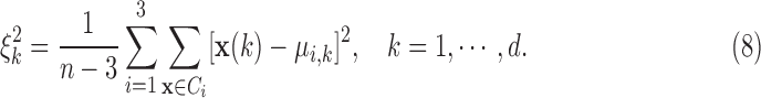
The proposed classification scheme can be described as follows. First, we select an ROI sub-network and formulate the feature vectors by calculating the Pearson correlation coefficients between all pairs of ROIs. In this paper, we formulate the ROI sub-network by selecting regions within the default mode network (DMN), which denotes the network of brain regions that are active when the brain is at the resting state [22]. Previous resting-state fMRI studies have demonstrated that the DMN is affected by AD [23]–[26]. More specifically, in this paper, we select the right and left hippocampi and isthmus of the cingulate cortices (ICCs) (4 regions) as our ROI sub-network. This is because that both hippocampus and ICC are part of the DMN, and can be well defined anatomically through the FreeSurfer software [26], even in brains with abnormal anatomy [25]. It has also been demonstrated in [25] that the functional connection between hippocampus and ICC was reduced in AD. Second, we propose a regularized linear discriminant analysis (LDA) approach, where we take shrinkage based regularization procedures to reduce the noise effect (including both biological variability and measurement errors) due to limited sample size. The feature vectors are then projected onto a one-dimensional axis using the proposed regularized LDA, where the differences between AD, MCI and NC subjects are maximized. Based on the Central Limit Theorem, we show that when used for fMRI based brain functioning classification, LDA is equivalent to the optimal maximum likelihood based classification method. Finally, a decision tree based multi-class AdaBoost classifier, which is robust to noise effect, is applied to the projected one-dimensional vectors to carry out the classification task.
The major results of this paper can be summarized as:
-
1)
We propose a regularized LDA approach, which aims to reduce the noise effect by using two shrinkage methods. The first shrinkage method moves the estimated mean of each class towards the overall mean, and the second one shifts the estimated covariance matrix for each class towards the identity matrix. Numerical analysis shows that: in comparison with the original LDA approach [27], the regularized LDA can reduce the noise effect and increase the classification accuracy significantly.
-
2)
We investigate the relationship between LDA-based and Maximum Likelihood (ML) based classification or decision making methods. Recall that LDA aims to separate two or more classes by projecting them into a subspace or direction where different classes show most significant differences [27]. In this paper, we prove that when the original data are normally distributed, LDA is equivalent to maximizing the log-likelihood function of the projected data. Note that there are millions of neurons within one fMRI voxel, according to the Central Limit Theorem, the overall fMRI signal corresponding to each voxel follows the normal distribution approximately. This implies that when used for fMRI based brain functioning classification, LDA is equivalent to the optimal ML based classification method.
-
3)
We conduct the connectivity pattern classification of AD, MCI and NC subjects by applying the regularized LDA and AdaBoost classifier based approach. First, we calculate the Pearson correlation coefficients between all possible pairs of the ROIs within the group to formulate the feature vectors. Second, the feature vectors are then projected onto a one-dimensional axis using the proposed regularized LDA, where the differences between AD, MCI and NC subjects are maximized. Finally, we construct the decision tree based on the projected feature vectors and carry out the classification using the multi-class AdaBoost classifier.
In this paper, we choose to utilize the AdaBoost classifier instead of the naive Bayesian classifier, since it has been observed consistently in literature that: the AdaBoost classifier could achieve significantly higher classification accuracy than the naive Bayesian classifier when the sample size is very limited [28]. Our numerical results demonstrate that: (i) LDA-Bayesian classifier can achieve a three-category (AD, MCI and NC) classification accuracy of 42%; (ii) LDA-AdaBoost classifier can increase the accuracy to 69%; (iii) when AdaBoost is combined with the regularized LDA, the accuracy can be further increased to 75%.
As expected, it is also observed that compared with AD and NC subjects, it is more difficult for the classifier to identify MCI subjects. The classification accuracy for AD and NC are as high as 80% and 83%, respectively, while the accuracy for MCI is only 63%. Our analysis also confirms the previous findings that the hippocampus and the isthmus of the cingulate cortex are closely involved in the development of AD and MCI [25].
The rest of this paper is organized as follows. In Section II, we present the proposed regularized LDA approach, and explore the relationship between LDA based and the Maximum Likelihood based classification methods. In Section III, we describe the ROI sub-network formulation, and elaborate how to perform AD, MCI and NC classification through connectivity pattern analysis. In Section IV we present the numerical results, and we conclude in Section V.
II. Regularized Linear DISCRIMINANT Analysis
In this section, first, we revisit the Linear Discriminant Analysis method. Second, we integrate two shrinkage methods with the original LDA to formulate the regularized LDA. Finally, we investigate the relationship between LDA and the ML estimation method.
A. Linear Discriminant Analysis
Linear Discriminant Analysis aims to separate two or more classes by projecting them into a subspace or direction where different classes show most significant differences [27]. LDA is a general framework that can be applied to classification problems with two or more classes. Here, we are considering the classification of three different groups: AD, MCI and normal subjects. Without loss of generality, we illustrate the basic idea of LDA using the three-class case. Suppose we have a set of  dimensional vector samples
  , where
  of them are from the first class, denoted as
  , and
, and  of them are from the second class, denoted as
  , and the remaining
  of them are from the third class, denoted as
  . For
. For  , the mean and scatter matrix (i.e., the scaled covariance matrix) of each of the three classes are defined as:
 |
Consider the projection of vectors in  to a new
  dimensional space:
 |
where  is a
is a  matrix to be determined by the LDA algorithm. In this paper, we only utilize the first dimension
  of projected vector
  where the differences among three classes are maximized. As a result, Equation (3) can be rewritten as:
 |
where  is the first row of the matrix
  . For
. For  , let
, let
 |
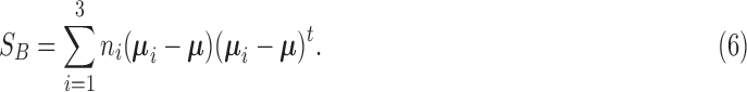
Define  as the overall mean,
  as the within-class scatter matrix, and the between-class scatter matrix
  as:
as:
 |
LDA seeks a transform vector  that maximizes the following objective function:
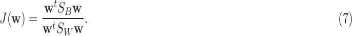 |
It can be proved [8] that Equation (7) can be maximized when  is the eigenvector corresponding to the largest eigenvalue of the matrix
  as
as  . As will be shown in Section 3, various classifiers, such as the Bayesian classifier and the AdaBoost classifier can then be applied to the projected vectors
  for further classification.
B. Regularized LDA
The original LDA algorithm has been widely applied in supervised learning problems [8]. However, as mentioned earlier, when the total number of subjects is small, the estimated statistics suffer considerably from the noise effect caused by both biological variability and measurement error, leading to low classification accuracy. For our fMRI based AD, MCI and NC classification, due to the very limited sample size, LDA together with the Bayesian classifier could only achieve an accuracy that is under 50%. To reduce the noise effect, we propose to regulate the original LDA using two shrinkage methods.
1). Shrinkage of the Mean
The first shrinkage method, originally proposed by Tibshirani et al.
[29] for gene expression profiling, adjusts the estimated mean vectors. In our case, let  be the whole sample set. Recall that for any
  . For
. For  ,
,  , define
  , and
, and  , where
  and
and  . Let
. Let  , and
, and  . The algorithm first calculates the following variances:
 |
Then for  , and
, and  , the scaled distance of
  to the centroid
  is calculated as:
 |
where  . After that, the distance is shrunken as follows:
 |
where  is a positive step size determined through cross-validation [8]. Now based on Equation (9), the shrinkage is achieved as follows:
 |
As can be seen from (10) and (11), each dimension of  has been shrunken towards the overall mean. This shrinkage method is essentially based on the
  test between the mean of each class and the overall mean at every dimension. Recall that the
  score of two sets of random variables
  and
and  , which have the same standard deviation
  , is defined as:
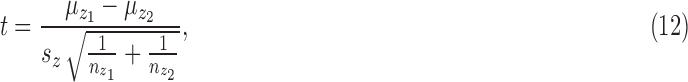 |
where  ,
,  , and
, and  and
and  are the sample sizes [30]. In this shrinkage method, for
  ,
,  , the
, the  score between each
  and
and  pair is defined as a distance in (9). If the distance
  is small, i.e., if
  , then most likely it is caused by the noise effect. In this case, the shrinkage method forces
  to be zero, and therefore reduces the noise effect.
2). Shrinkage of the Covariance Matrix
The second shrinkage method, proposed by Friedman et al.
[31], regulates the estimation of covariance matrix  for each class as:
 |
where  is the identity matrix, and
  a positive number determined through cross-validation. The basic idea of this shrinkage method is that: when the sample size is small, the estimated covariance matrix
  , generally becomes non-invertible. By adding a small perturbation to the slightly scaled covariance matrix, the adjusted or shrunken
  will generally become invertible as expected.
After the regularized LDA transform, the feature vectors are projected into a set of real valued numbers. After that, a selected classifier can be applied to the transformed data for further classification.
C. LDA and the Ml Estimation
In this subsection, we demonstrate that when the original data from all classes are normally distributed, then LDA is equivalent to the ML method. For  , assume each vector
  in class
  has the same probability density function (pdf):
 |
Consider a general linear transform defined by:
 |
where  is a
is a  matrix. For the transformed data, the probability density function becomes:
 |
where  ,
,  , and
, and 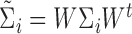 .
.
Recall that in LDA, we try to find  such that the difference among different classes is maximized in the transformed space. Without loss of generality, we assume that the major difference lies in the first dimension of the transformed vector
  only, and the remaining
  dimensions make little contributions. Under this assumption,
  and
and  can be decomposed as:
 |
since for each  ,
,  ,
,  . Accordingly, the matrix
  can also be decomposed as
 |
In this case, we have  ,
,  ,
,  and
and  .
.
For fairness, in LDA based classification, the sample size of the three classes is assumed to be the same, i.e.,  . With the probability density function given in (16), the log-likelihood function of the original data can be written as:
 |
To find the optimal  that maximizes
  , set
, set  and
and  , we get:
 |
Substitute (20) and (21) into (19) and remove the constant items, the optimization of  is equivalent to optimizing the following function:
 |
The optimal choice of  will satisfy the differential equation:
 |
It was shown in [8] that the partial differential equations are satisfied when  is composed of eigenvectors of the matrix
  .
.
If we only keep the eigenvector corresponding to the largest eigenvalue of  , then we obtain the LDA algorithm presented in Section II-A. As can be seen, LDA is equivalent to the ML method.
III. Classification of Ad, MCI and NC Subjects Based on Connectivity Pattern Analysis
In this section, we formulate the ROI sub-network, and perform AD, MCI and NC Subjects classification through connectivity pattern analysis, by exploiting the proposed Regularized LDA.
A. ROI Sub-Network
The default mode network (DMN) is one of the well studied networks at the resting state [22]. Previous resting-state fMRI studies have demonstrated that the DMN is affected by AD [23]–[26]. Both hippocampus and ICC are part of the DMN, and can be well defined anatomically through the FreeSurfer software [26], even in brains with abnormal anatomy [25]. The paper by Zhu et al. [25] specifically demonstrated that the functional connection between hippocampus and ICC was reduced in AD.
Motivated by the observations above, in this paper, we select the right and left hippocampi and ICCs (4 regions) as our ROI sub-network. Our connectivity pattern analysis is carried out following the procedure below.
First, we calculate the Pearson correlation coefficients between all possible pairs of the ROIs within the group to formulate the feature vectors. As we now have 4 regions in the ROI sub-network, for each subject  , we can obtain a
  dimensional (
 ) vector
  , consisting of the Pearson correlation coefficients for each pair of ROIs. When we have
  subjects, we get the feature vector set
  .
.
Second, using the proposed regularized LDA, we map  to a one-dimensional subspace or axis, where the differences between AD, MCI and NC subjects are maximized, and denote the projected vectors as
  .
.
Finally, we construct the decision trees based on  and carry out the classification using the multi-class AdaBoost classifier.
In the following subsections, we will provide more details on decision tree construction, and multi-class classification using AdaBoost.
B. Basic Decision Tree Construction
In the classification procedure, we will construct  basic decision trees. Each decision tree divides the LDA projected data set
  , into
  regions, and each region is called a leaf node. Here, the number of regions,
  , and the boundaries for all the regions are chosen by the decision tree algorithm to minimize the Gini impurity coefficient
  [32]. More specifically, assume
  , where
  . Here
  denote the projected data set corresponding to AD, MCI and NC subjects, respectively. For
  , without loss of generality, suppose
  data samples
  are assigned to node
  , where
  ,
,  . The Gini impurity coefficient of node
  is calculated as:
 |
where  and
and  .
.
For any given input  to be classified, if
  falls within the boundaries of node
  , then it will be assigned to node
  , and paired with the majority class inside this node. Note that in our case,
  , are all real-valued numbers. That is,
  . In this case, the boundary between two neighboring regions is reduced to a point, and hence each region corresponds to an interval on the
  axis.
axis.
The decision tree is a weak classifier. In most applications, it needs to be incorporated with an ensemble classifier to achieve higher accuracy. Some representative ensemble algorithms include Bagging and Boosting [32]. In the following, we will apply the AdaBoost algorithm to construct the ensemble classifier, due to its robustness under noise effect [8], [28].
C. The Multi-Class
The multi-class AdaBoost classifier is built upon an ensemble of weak decision tree classifiers [28]. Given a set of labeled data  , where
  , the algorithm first starts with an empty ensemble and
  decision trees, as constructed above. Each sample
  in the data set is given an initial weight
  , where
  . Then for
  , the algorithm will iteratively implement the following procedures:
1). Weighted Classification Error Calculation
Apply a weak decision tree classifier  to the samples and calculate the weighted classification error. More specifically, let
 |
where  is the assigned class for sample
  , and
, and  is the true class
  belongs to. Then the weighted classification error
  would be
 |
2). Voting Weight Assignment
Based on the weighted classification error  , the algorithm will assign a voting weight
  for the weak decision tree classifier
  as follows:
 |
and then add classifier  into the ensemble.
3). Weight Update
Before the next iteration, the weight of each data sample  is updated as follows:
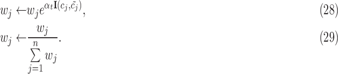 |
The procedure in (29) ensures that the weights  , form a probability distribution with
 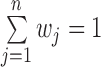 . As can be seen, after the update, those samples which have been incorrectly classified in current iteration will have higher weights in the next iteration.
4). Final Classification
After  iterations, there will be
  decision trees in the ensemble. The final classification is a weighted majority votes of each of those classifiers.
As will be shown in the next Section, the combination of regularized LDA and AdaBoost can achieve much higher accuracy in AD, MCI and NC classification than the conventional approach based on the original LDA and the Bayesian classifier.
IV. Numerical Analysis
A. FMRI Data Acquisition and Pre-Processing
1). Subjects
Ten patients with mild-to-moderate probable AD, 11 MCI patients, and 12 age- and education- matched healthy NC subjects were recruited to participate in this study. The study was approved by the Michigan State University Institutional Review Board. All subjects or their legal representatives provided written informed consent. All subjects were carefully screened to exclude those with a history of stroke, brain tumors, aneurysms, brain surgery, serious head injury, or other significant neurological disease, as well as those with uncontrolled diabetes, hypertension, and hypothyroidism. All subjects were also screened for MR-incompatible metallic implants. NC subjects were community-dwelling older adults recruited from the Greater Lansing area in Michigan. The AD and MCI patients were recruited through the Memory Disorders Clinic in the Department of Neurology at Michigan State University and were diagnosed using standard criteria by a practicing neurologist (NINCDS-ADRDA criteria for clinically probable AD and Petersen criteria for MCI).
2). fMRI Data Acquisition
The MRI experiment was conducted on a GE 3T Signa® HDx MR scanner (GE Healthcare, Waukesha, WI) with an 8-channel head coil. During each session, first and higher-order shimming procedures were carried out to improve magnetic field homogeneity. To study resting-state brain function, echo-planar images, starting from the most inferior regions of the brain, were acquired for 7 minutes with the follow- ing parameters: 38 contiguous 3-mm axial slices in an interleaved order, time of echo  ms, time of repetition
  ms, flip
  , field of view
  cm, matrix
  , ramp sampling, and with the first four data points discarded. Each volume of slices was acquired 164 times while a subject was asked to relax and keep his/her eyes open in a dim-light condition. After the functional data acquisition, diffusion-weighted images were acquired with a dual spin-echo echo-planar imaging (EPI) sequence for 12 minutes and 6 seconds with the following parameters: 48 contiguous 2.4-mm axial slices in an interleaved order,
  cm
cm cm, matrix
  , number of excitations
  ,
,  ms,
ms,  s, 25 diffusion-weighted volumes (one per gradient direction) with
  s/mm2, one volume with
  and parallel imaging acceleration
  . Finally, 180 T1-weighted 1-mm3 isotropic volumetric inversion recovery fast spoiled gradient-recalled images (10 minute scan time), with cerebrospinal fluid (CSF) suppressed, were obtained to cover the whole brain with the following parameters:
  ms, TR of
  ms, time of inversion
  ms, TR of
  ms, flip
  ,
,  cm, matrix
  , slice
  mm, and receiver
  kHz.
kHz.
3). Resting-State fMRI Individual-Subject Data Pre-Processing
For each subject, the acquisition timing difference was first corrected for different slice locations. With the last functional volume as the reference, rigid-body motion correction was done in three translational and three rotational directions. The amount of motion was estimated and then modeled in data analysis. For each subject, spatial blurring with a full width half maximum (FWHM) of 4mm was used to reduce random noise and inter-subject anatomical variation during group analysis. At each voxel, motion-estimation parameters, baseline, linear and quadratic system-induced signal trends were removed from the time courses using the “3dDeconvolve” routine in AFNI. Brain global and CSF mean signals were modeled as nuisance variables and removed from the time courses as well. In order to create the time course from pure CSF regions, the lateral and 3rd ventricles on the high-resolution T1-weighted volumetric images were segmented using FreeSurfer software followed by 1 mm3 erosion. The cleaned time courses were then band-pass filtered in the range of 0.009 Hz - 0.08 Hz and used for connectivity analyses.
B. Generation of ROIs for Connectivity Analyses
We selected relatively small-size, anatomically-defined regions based on the FreeSurfer [26] segmentation as seeds for connectivity analyses in this work, including right and left isthmi of the cingulate cortex (ICCs), and right and left hippocampi. Each of these regions is well-defined by FreeSurfer, with reasonable volumes for connectivity analyses (means of 2089/2381  for the right/left ICCs and 3494/3400
  for the right/left hippocampi for the NC group). The ICCs defined in FreeSurfer overlaps with the boundaries of the PCC/RSC (L1, P50, S26), defined by Buckner et al.
[33] for their connectivity analyses of the DMN. The right and left hippocampi are also part of the DMN [33] and are known to be affected by AD.
for the right/left hippocampi for the NC group). The ICCs defined in FreeSurfer overlaps with the boundaries of the PCC/RSC (L1, P50, S26), defined by Buckner et al.
[33] for their connectivity analyses of the DMN. The right and left hippocampi are also part of the DMN [33] and are known to be affected by AD.
C. Performance Comparison of Different Classification Algorithms
In this subsection, we present the classification performance of the proposed method and compare it to existing methods. The performance of the classifier is evaluated using the Leave-One-Out (LOO) cross-validation. As was pointed out in [21], comparing with other method, LOO might have a higher estimate error. However, in our study, as the size of data sample is small, splitting the data into two sets based on a threshold would generate a biased testing set which contains only a few subjects for each category. That is why LOO is chosen to evaluate the performance of the classifiers in this case. As described earlier, the ROIs used are the hippocampus and ICC from both hemispheres of the brain.
Table 1 shows the performance of five classifiers. In the first one, a naive Bayesian classifier is employed after the original LDA transform. As can be seen, its final accuracy is only 42.4%. As explained in Section 2, the main reason of such an unsatisfying performance is that: when the number of data samples is small, the estimation of class means and covariance matrices in LDA suffers from severe noise effect, leading to overfitting. In the second one, the original LDA is combined with the AdaBoost classifier. As can be seen, the accuracy is increased to 69.7% by AdaBoost. The accuracies corresponding to Logistic Regression (LR) and Support Vector Machine (SVM) are 36.4% and 57.6%, respectively. The last one is the regularized LDA combined with the AdaBoost classifier that we proposed. The shrinkage operations in the regularized LDA can reduce the noise effect in the estimation, and further improve the accuracy to 75.8%. As can be seen, Clearly, the purposed method is shown to be more robust in distinguishing AD, MCI and NC subjects. Compared to existing fMRI based classification algorithms [5], [6], i.e., LDA with Bayesian classifier, the proposed method has improved the classification accuracy by 33.4% with a p-value of 0.007 using the McNemar test [34].
TABLE 1. Comparison of 3-Category (AD, MCI, NC) cLassification Results.
| Method | Accuracy |
|---|---|
| LDA with Bayesian | 42.4% |
| LDA with AdaBoost | 69.7% |
| LR with L2 penalty | 36.4% |
| SVM with RBF kernel | 57.6% |
| Regularized LDA with AdaBoost | 75.8% |
Table 2 to VI show the confusion matrices of the five classifiers. It can be seen that the purposed method shows better performance in terms of precision and recall rates. Also, as expected, compared with NC subjects and AD patients, it is generally more difficult for the classifier to identify MCI patients, and the classification accuracy for MCI patients is much lower than that for AD and NC subjects. MCI is a transitional stage of dementia between NC and AD. Therefore, MCI patients generally share some similar characteristics in functional brain connectivities with AD patients or NC subjects. As a result, the classification algorithm is prone to mis-recognize MCI patients as AD or NC subjects.
TABLE 3. LDA with AdaBoost.
| Predicted Class | Recall | ||||
|---|---|---|---|---|---|
| NC | MCI | AD | |||
| Actual Class | NC | 9 | 2 | 1 | 75.0% |
| MCI | 2 | 7 | 2 | 63.6% | |
| AD | 2 | 1 | 7 | 70.0% | |
| Precision | 69.2% | 70.0% | 70.0% | ||
TABLE 4. LR With L2 Penalty.
| Predicted Class | Recall | ||||
|---|---|---|---|---|---|
| NC | MCI | AD | |||
| Actual Class | NC | 6 | 3 | 3 | 50.0% |
| MCI | 7 | 2 | 2 | 18.2% | |
| AD | 2 | 4 | 4 | 40.0% | |
| Precision | 40.0% | 22.2% | 44.4% | ||
TABLE 5. SVM With RBF Kernel.
| Predicted Class | Recall | ||||
|---|---|---|---|---|---|
| NC | MCI | AD | |||
| Actual Class | NC | 7 | 5 | 0 | 58.3% |
| MCI | 2 | 8 | 1 | 72.7% | |
| AD | 1 | 5 | 4 | 40.0% | |
| Precision | 70.0% | 44.4% | 80.0% | ||
TABLE 6. Regularized LDA With AdaBoost.
| Predicted Class | Recall | ||||
|---|---|---|---|---|---|
| NC | MCI | AD | |||
| Actual Class | NC | 10 | 2 | 0 | 83.3% |
| MCI | 2 | 7 | 2 | 63.6% | |
| AD | 1 | 1 | 8 | 80.0% | |
| Precision | 76.9% | 70.0% | 80.0% | ||
TABLE 2. LDA With Bayesian.
| Predicted Class | Recall | ||||
|---|---|---|---|---|---|
| NC | MCI | AD | |||
| Actual Class | NC | 6 | 5 | 1 | 50.0% |
| MCI | 6 | 4 | 1 | 36.4% | |
| AD | 2 | 4 | 4 | 40.0% | |
| Precision | 42.9% | 30.8% | 66.7% | ||
V. Conclusions
This paper proposes a reliable method for AD, MCI and NC subject classification that is highly robust under size limited fMRI data samples, by exploiting brain network connectivity pattern analysis. To do it, first, we selected the right and left hippocampi regions and isthmus of the cingulate cortices (ICCs) as our ROI sub-network, and calculated the Pearson correlation coefficients between all possible ROI pairs and used them to form a feature vector for each subject. Second, the vectors were projected into a one-dimensional axis using the proposed regularized LDA approach, where the differences between AD, MCI and NC subjects were maximized. Shrinkage based regularization procedures were taken to reduce the noise effect due to the limited sample size. Finally, a decision tree based multi-class AdaBoost classifier, which is robust to noise effect, was applied to the projected one-dimensional vectors to perform the classification.
Both the theoretical and numerical analysis demonstrated that: (i) the regularization methods and the AdaBoost classifier can increase the classification accuracy significantly; (ii) brain network connectivity analysis, which evaluates the changes in the pattern of connectivity among multiple or all regions in the sub-network, can reveal in-depth information about brain connectivity and result in relatively accurate classification of AD, MCI and NC, especially when the sample size is very limited; (iii) our analysis confirms the previous findings that the hippocampus and the isthmus of the cingulate cortex are closely involved in the development of AD and MCI.
Potentially, the proposed framework can be applied to other classification problems as well, especially under limited sample size.
Funding Statement
This work was supported by the National Science Foundation under Award ECCS-1744604.
References
- [1].Morris J. C.et al. , “Mild cognitive impairment represents early-stage Alzheimer disease,” Arch. Neurol., vol. 58, no. 3, pp. 397–405, 2001. [DOI] [PubMed] [Google Scholar]
- [2].Westman E., Muehlboeck J.-S., and Simmons A., “Combining MRI and CSF measures for classification of Alzheimer’s disease and prediction of mild cognitive impairment conversion,” Neuroimage, vol. 62, no. 1, pp. 229–238, 2012. [DOI] [PubMed] [Google Scholar]
- [3].Lehmann C.et al. , “Application and comparison of classification algorithms for recognition of Alzheimer’s disease in electrical brain activity (EEG),” J. Neurosci. Methods, vol. 161, no. 2, pp. 342–350, 2007. [DOI] [PubMed] [Google Scholar]
- [4].Cuingnet R.et al. , “Automatic classification of patients with Alzheimer’s disease from structural MRI: A comparison of ten methods using the ADNI database,” NeuroImage, vol. 56, no. 2, pp. 766–781, 2011. [DOI] [PubMed] [Google Scholar]
- [5].Wang K.et al. , “Discriminative analysis of early Alzheimer’s disease based on two intrinsically anti-correlated networks with resting-state fMRI,” in Proc. Int. Conf. Med. Image Comput. Comput.-Assist. Intervent., 2006, pp. 340–347. [DOI] [PubMed] [Google Scholar]
- [6].Chen G.et al. , “Classification of Alzheimer disease, mild cognitive impairment, and normal cognitive status with large-scale network analysis based on resting-state functional MR imaging,” Radiology, vol. 259, no. 1, pp. 213–221, 2011. [DOI] [PMC free article] [PubMed] [Google Scholar]
- [7].Pritchard W. S.et al. , “EEG-based, neural-net predictive classification of Alzheimer’s disease versus control subjects is augmented by non-linear EEG measures,” Electroencephalogr. Clin. Neurophysiol., vol. 91, no. 2, pp. 118–130, 1994. [DOI] [PubMed] [Google Scholar]
- [8].Stork D. G., Hart P. E., and Duda R. O., Pattern Classification. Hoboken, NJ, USA: Wiley, 2012. [Google Scholar]
- [9].Magnin B.et al. , “Support vector machine-based classification of Alzheimer’s disease from whole-brain anatomical MRI,” Neuroradiology, vol. 51, no. 2, pp. 73–83, 2009. [DOI] [PubMed] [Google Scholar]
- [10].Korolev I. O., Symonds L. L., and Bozoki A. C., “Predicting progression from mild cognitive impairment to Alzheimer’s dementia using clinical, MRI, and plasma biomarkers via probabilistic pattern classification,” PLoS One, vol. 11, no. 2, p. e0138866, 2016. [DOI] [PMC free article] [PubMed] [Google Scholar]
- [11].Challis E., Hurley P., Serra L., Bozzali M., Oliver S., and Cercignani M., “Gaussian process classification of Alzheimer’s disease and mild cognitive impairment from resting-state fMRI,” NeuroImage, vol. 112, pp. 232–243, May 2015. [DOI] [PubMed] [Google Scholar]
- [12].Jie B., Zhang D., Gao W., Wang Q., Wee C.-Y., and Shen D., “Integration of network topological and connectivity properties for neuroimaging classification,” IEEE Trans. Biomed. Eng., vol. 61, no. 2, pp. 576–589, Feb. 2014. [DOI] [PMC free article] [PubMed] [Google Scholar]
- [13].Khazaee A., Ebrahimzadeh A., and Babajani-Feremi A., “Identifying patients with Alzheimer’s disease using resting-state fMRI and graph theory,” Clin. Neurophysiol., vol. 126, no. 11, pp. 2132–2141, Nov. 2015. [DOI] [PubMed] [Google Scholar]
- [14].Wee C.-Y.et al. , “Identification of MCI individuals using structural and functional connectivity networks,” NeuroImage, vol. 59, no. 3, pp. 2045–2056, 2012. [DOI] [PMC free article] [PubMed] [Google Scholar]
- [15].Zhang D., Wang Y., Zhou L., Yuan H., and Shen D., “Multimodal classification of Alzheimer’s disease and mild cognitive impairment,” NeuroImage, vol. 55, no. 3, pp. 856–867, 2011. [DOI] [PMC free article] [PubMed] [Google Scholar]
- [16].Liu F., Zhou L., Shen C., and Yin J., “Multiple kernel learning in the primal for multimodal alzheimer’s disease classification,” IEEE J. Biomed. Health Inform., vol. 18, no. 3, pp. 984–990, May 2014. [DOI] [PubMed] [Google Scholar]
- [17].Xu L.et al. , “Prediction of progressive mild cognitive impairment by multi-modal neuroimaging biomarkers,” J. Alzheimer’s Disease, vol. 51, no. 4, pp. 1045–1056, 2016. [DOI] [PubMed] [Google Scholar]
- [18].Li Q., Wu X., Xu L., Chen K., Yao L., and Li R., “Multi-modal discriminative dictionary learning for Alzheimer’s disease and mild cognitive impairment,” Comput. Methods Programs Biomed., vol. 150, pp. 1–8, Oct. 2017. [DOI] [PubMed] [Google Scholar]
- [19].Li Q., Wu X., Xu L., Chen K., and Yao L., “Classification of Alzheimer’s disease, mild cognitive impairment, and cognitively unimpaired individuals using multi-feature kernel discriminant dictionary learning,” Frontiers Comput. Neurosci., vol. 11, p. 117, Jan. 2017. [DOI] [PMC free article] [PubMed] [Google Scholar]
- [20].Rathore S., Habes M., Iftikhar M. A., Shacklett A., and Davatzikos C., “A review on neuroimaging-based classification studies and associated feature extraction methods for Alzheimer’s disease and its prodromal stages,” NeuroImage, vol. 155, pp. 530–548, Jul. 2017. [DOI] [PMC free article] [PubMed] [Google Scholar]
- [21].Varoquaux G., “Cross-validation failure: Small sample sizes lead to large error bars,” NeuroImage, vol. 180, pp. 68–77, Oct. 2018. [DOI] [PubMed] [Google Scholar]
- [22].Buckner R. L.et al. , “The organization of the human cerebellum estimated by intrinsic functional connectivity,” J. Neurophysiol., vol. 106, no. 5, pp. 2322–2345, 2011. [DOI] [PMC free article] [PubMed] [Google Scholar]
- [23].Greicius M. D., Srivastava G., Reiss A. L., and Menon V., “Default-mode network activity distinguishes Alzheimer’s disease from healthy aging: Evidence from functional MRI,” Proc. Nat. Acad. Sci. USA, vol. 101, no. 13, pp. 4637–4642, 2004. [DOI] [PMC free article] [PubMed] [Google Scholar]
- [24].Zhang H.-Y.et al. , “Resting brain connectivity: Changes during the progress of Alzheimer disease,” Radiology, vol. 256, no. 2, pp. 598–606, 2010. [DOI] [PubMed] [Google Scholar]
- [25].Zhu D. C., Majumdar S., Korolev I. O., Berger K. L., and Bozoki A. C., “Alzheimer’s disease and amnestic mild cognitive impairment weaken connections within the default-mode network: A multi-modal imaging study,” J. Alzheimer’s Disease, vol. 34, no. 4, pp. 969–984, 2013. [DOI] [PubMed] [Google Scholar]
- [26].Fischl B.et al. , “Whole brain segmentation: Automated labeling of neuroanatomical structures in the human brain,” Neuron, vol. 33, no. 3, pp. 341–355, 2002. [DOI] [PubMed] [Google Scholar]
- [27].Fisher R. A., “The use of multiple measurements in taxonomic problems,” Ann. Eugenics, vol. 7, no. 2, pp. 179–188, 1936. [Google Scholar]
- [28].Zhu J., Zou H., Rosset S., and Hastie T., “Multi-class AdaBoost,” Statist. Interface, vol. 2, no. 3, pp. 349–360, 2009. [Google Scholar]
- [29].Tibshirani R., Hastie T., Narasimhan B., and Chu G., “Diagnosis of multiple cancer types by shrunken centroids of gene expression,” Proc. Nat. Acad. Sci. USA, vol. 99, no. 10, pp. 6567–6572, 2002. [DOI] [PMC free article] [PubMed] [Google Scholar]
- [30].Rice J. A., Mathematical Statistics and Data Analysis. Boston, MA, USA: Cengage, 2006. [Google Scholar]
- [31].Friedman J. H., “Regularized discriminant analysis,” J. Amer. Statist. Assoc., vol. 84, no. 405, pp. 165–175, 1989. [Google Scholar]
- [32].Zhou Z.-H., Ensemble Methods: Foundations and Algorithms. Boca Raton, FL, USA: CRC Press, 2012. [Google Scholar]
- [33].Buckner R. L., Andrews-Hanna J. R., and Schacter D. L., “The brain’s default network-anatomy, function, and relevance to disease,” Year Cogn. Neurosci., vol. 1, pp. 1124–1138, 2008. [DOI] [PubMed] [Google Scholar]
- [34].Kuncheva L. I., Combining Pattern Classifiers: Methods and Algorithms. Jul. 2004.