Randomly distributed embedding making short-term high-dimensional data predictable

Significance

Making accurate forecast or prediction is a challenging task in the big data era, in particular for those datasets involving high-dimensional variables but short-term time series points, and these datasets are omnipresent in many fields. In this work, a model-free framework, named as “randomly distributed embedding” (RDE), is proposed to accurately predict future dynamics based on such short-term but high-dimensional data. The RDE framework creates the distribution information from the interactions among high-dimensional variables to compensate for the lack of time points in real applications. Instead of roughly predicting a single trial of future values, this framework achieves the accurate prediction by using the distribution information.

Abstract

Future state prediction for nonlinear dynamical systems is a challenging task, particularly when only a few time series samples for high-dimensional variables are available from real-world systems. In this work, we propose a model-free framework, named randomly distributed embedding (RDE), to achieve accurate future state prediction based on short-term high-dimensional data. Specifically, from the observed data of high-dimensional variables, the RDE framework randomly generates a sufficient number of low-dimensional “nondelay embeddings” and maps each of them to a “delay embedding,” which is constructed from the data of a to be predicted target variable. Any of these mappings can perform as a low-dimensional weak predictor for future state prediction, and all of such mappings generate a distribution of predicted future states. This distribution actually patches all pieces of association information from various embeddings unbiasedly or biasedly into the whole dynamics of the target variable, which after operated by appropriate estimation strategies, creates a stronger predictor for achieving prediction in a more reliable and robust form. Through applying the RDE framework to data from both representative models and real-world systems, we reveal that a high-dimension feature is no longer an obstacle but a source of information crucial to accurate prediction for short-term data, even under noise deterioration.

The big data era has witnessed the accumulation of various types of time series data from microscopic gene expression data through mesoscopic neural activity data to macroscopic ecological or/and atmosphere data (1–5). A challenging task is making accurate forecast or prediction (6, 7) based on such time series datasets, in particular for those datasets with short-term time points but high-dimensional variables. Generally, these two properties are both considered as obstacles for accurate and robust prediction, because short-term datasets always result in fewer statistical patterns for prediction while high-dimensional system variables are likely to bring the curse of dimensionality problem. Specifically, for the model-based methods, such as regression methods (8), or equation-based models (9, 10), taking account of higher-dimensional variables requires a larger number of parameters or weights in the model, making it impractical to estimate these parameters or weights accurately only with short-term data. For the model-free methods, such as the empiricism-based methods where the nearest neighbors in historical data are used to predict the future values (11, 12), short-term data make the depicted attractor sparse in a high-dimensional space, which therefore, yields a problem of the false nearest neighbors. Additionally, machine learning methods, including deep belief network (13), long short-term memory network (14), and reservoir computing (15–18), have been intensively studied and applied to achieve systems reconstructions and dynamics prediction (19–26). However, based on the neural networks framework (27, 28), the performance of the artificial neural networks crucially and largely relies on the length of the available training data. Thus, these representative methods are effective in accurate prediction only when the training set contains a sufficiently large amount of training data. To handle high-dimensional data, dimension reduction techniques [e.g., various principal component analyses (29, 30), sparse regularization (31–33), and local linearizations] are usually applied for feature extraction. However, the consequence of these applications is likely to overlook interactions (particularly nonlinear interactions) or associations mutually between variables in high-dimensional systems. These interactions in nonlinear dynamics are the crucial information for prediction, remedying the difficulty due to the limited length of observed data, and therefore, the reduction techniques are not always beneficial to accurate prediction of dynamics in complex nonlinear systems (34). Thus, making a good use of the deterministic association or interaction information among the high-dimensional variables becomes a pivotal key to designing a useful prediction method (35).

In this work, we propose a model-free framework, named as randomly distributed embedding (RDE), to accurately predict future dynamics based on the observed short-term high-dimensional data. In addition to using the temporal information of each variable, such as the traditional methods usually execute for the long-term data, we exploit the spatial information of the short-term data, such as associations or interactions among the high-dimensional variables. Particularly, the RDE framework can be thought of as an exchange scheme between the spatial information among the observed high-dimensional variables and the time-dependent probability distributions for the temporal dynamics. Thus, it improves the predictability significantly for a target variable. By using the RDE framework to the short-term high-dimensional data produced by both representative models and real-world systems, we show that a high-dimensional feature is no longer an obstacle but a source of information crucial to accurate prediction for short-term data even under noise perturbation.

RDE Framework

Delay and Nondelay Embeddings Form Low-Dimensional Attractors.

Usually in a typical high-dimensional nonlinear system, there is a large number of variables interacting with each other; however, the steady dynamics after a transient phase is generally constrained into a low-dimensional subspace due to dissipation. Thus, the state-space technique, based on the embedding theorem, makes it possible to reconstruct a low-dimensional attractor from time series data observed from such a system (36, 37).

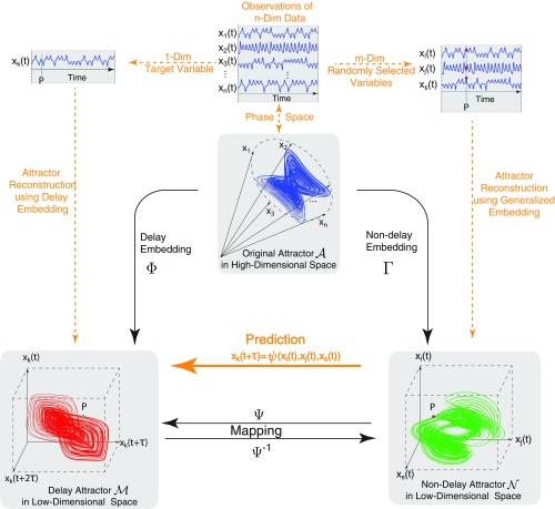
As particularly shown in Fig. 1, with the $n$-dimensional time series data $x_i\left(t\right),i=\mathrm{1,2},\dots ,n$, two kinds of 3D (three-dimensional) attractors can be reconstructed. Specifically, according to the delayed embedding theory (36, 37), one kind is reconstructed in a form of $\mathcal{M}\left(x_k\left(t\right),x_k\left(t+\tau \right),x_k\left(t+2\tau \right)\right)$, where $x_k\left(t\right)$ is the observed time series of a single variable and also, the target variable to be predicted. The other kind, according to the generalized embedding theory (37–39), is formed by $\mathcal{N}\left(x_i\left(t\right),x_j\left(t\right),x_s\left(t\right)\right)$, where $x_i\left(t\right),x_j\left(t\right)$, and $x_s\left(t\right)$ are the observed time series of multivariables that are randomly selected and used to predict $x_k\left(t\right)$. To make the expression clear and compact, we name $\mathcal{M}$ as the delay attractor and $\mathcal{N}$ as the nondelay attractor.

Fig. 1.

Sketch of embedding the original attractor in a high-dimensional space into a reconstructed attractor in a low-dimensional space.

The dimension L for reconstructing the above attractors is equal to three, which is an example of the reconstructed space. In fact, the reconstructed dimension for a general attractor, based on the embedding theory (SI Appendix), could be either smaller or larger; however, it is usually much less than the high dimension of the original dissipative system. Thus, as conveyed by the embedding theory, these delay and nondelay attractors of lower dimensions theoretically preserve the dynamical information of the entire system in different ways. As illustrated in Fig. 1, the temporal (or delay) information of the target single variable is explored in the delay attractor while the spatial or association information among high-dimensional variables is mainly exploited in the nondelay attractor.

A Predictor: Mapping from Nondelay Attractor of Multivariables to Delay Attractor of One Target Variable.

The embedding theory reveals that all of the above reconstructed attractors with appropriately reconstructed dimensions are topologically conjugated to the original attractor because of a diffeomorphism map (i.e., $\mathrm{\Psi }:\mathcal{N}\to \mathcal{M}$) (37). Thus, for each index tuple $l=\left(i,j,s\right)$, a component of such a mapping, denoted by ${\psi }_l$, can be obtained as a predictor for the target variable $x_k\left(t\right)$ in the form of

$$x_k\left(t+\tau \right)={\psi }_l\left(x_i\left(t\right),x_j\left(t\right),x_s\left(t\right)\right).$$

Notice that $L=3$ is much lower than the dimension $n$ of the entire system. Then, typical approximation frameworks with usual fitting algorithms could be used to implement this predictor. In this paper, we apply the Gaussian Process Regression method (40) to fit each ${\psi }_l$. The above mapping actually transforms the association information among multivariables into the temporal dynamics of the predicted variable.

Multiple Predictors Forming a Probability Distribution at Each Future Time Point.

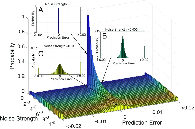
Provided with the observed high-dimensional data, we reconstruct nondelay attractors $\mathcal{N}\left(x_i\left(t\right),x_j\left(t\right),x_s\left(t\right)\right)$ as many as possible with different index tuples $l=\left(i,j,s\right)$. For each nondelay attractor, we can fit the corresponding predictor ${\psi }_l$ to predict a specific target variable $x_k\left(t\right)$. Here, each tuple $l=\left(i,j,s\right)$ is randomly chosen with replacement from any index combinations of variables in the original high-dimensional data. When the corresponding ${\psi }_l$ is obtained, one-step prediction ${\tilde{x}}_k^l\left(t^{*}+\tau \right)={\psi }_l\left(x_i\left(t^{*}\right),x_j\left(t^{*}\right),x_s\left(t^{*}\right)\right)$ could be further obtained where $t^{*}+\tau$ is the time instance to be predicted at time point $t^{*}$. Thus, the more variables of the original data that are experimentally observed, the more one-step prediction values, ${\tilde{x}}_k^l\left(t^{*}+\tau \right)$, for $x_k\left(t^{*}+\tau \right)$ can be obtained. From the fact that each nondelay embedding preserves the dynamical information of the entire system in a different way, these embeddings have different performances in making prediction, especially under noise deterioration. In fact, at each future time point, the multiple prediction values ${\tilde{x}}_k^l\left(t^{*}+\tau \right)$ actually form a probability (frequency) distribution, except for some degenerative tuples that appear as the outliers in the distribution of prediction as illustrated in Fig. 2 (Results and SI Appendix).

Fig. 2.

Distribution of prediction errors by random embedding under different noise levels for a benchmark model of a linear system. (A–C) Probability distributions under different noise strengths.

Distribution Leveraging Prediction Accuracy.

Compared with each single prediction, the above-obtained distribution renders more information leveraging prediction accuracy. Specifically, better prediction can be estimated by

$${\tilde{x}}_k\left(t^{*}+\tau \right)=\mathcal{E}\left[{\tilde{x}}_k^l\left(t^{*}+\tau \right)\right],$$

where $\mathcal{E}\left[\cdot \right]$ represents an estimation based on the available probability information of the random variable ${\tilde{x}}_k^l$. A straightforward scheme to obtain this estimation is to use the expectation of the distribution as the final prediction value [i.e., ${\tilde{x}}_k\left(t^{*}+\tau \right)=\int xp\left(x\right)\mathrm{d}x$, where $p\left(x\right)$ denotes the probability density function of the random variable ${\tilde{x}}_k^l$]. In fact, this expectation scheme is particularly useful for a general case where each random embedding yields a prediction error ${\delta }_l$, satisfying ${\tilde{x}}_k^l\left(t^{*}+\tau \right)=x_k\left(t^{*}+\tau \right)+{\delta }_l$ and becoming a random variable with an expectation very close to zero. However, when the prediction error expectation deviates far from zero, an aggregation scheme, independent of the zero-expectation assumption, has to be taken into account in the RDE framework. Concretely, in light of the feature bagging strategy in machine learning (41, 42), each random embedding is treated as a feature, and thus, the final prediction value is estimated by the aggregated average of the selected features: that is,

$${\tilde{x}}_k\left(t^{*}+\tau \right)=\sum _{i=1}^r{\omega }_i{\tilde{x}}_k^{l_i}\left(t^{*}+\tau \right),$$

where each ${\omega }_i$ is a weight related to the in-sample fitting error of ${\psi }_{l_i}$ and $r$ represents the number of the best embeddings showing fewer fitting errors for the final prediction (Materials and Methods).

RDE Algorithm.

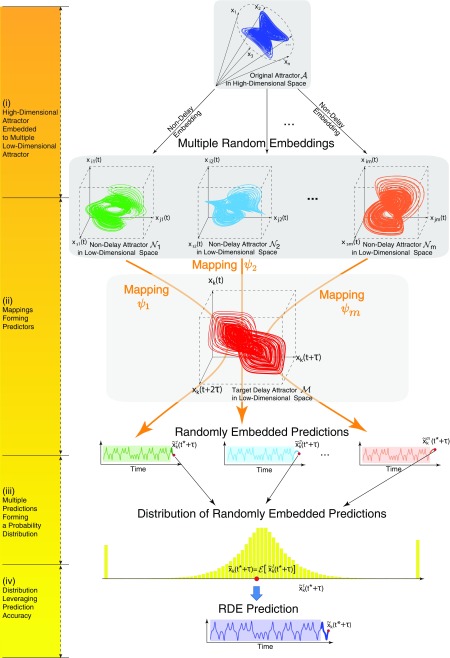
Altogether with the above settings, the RDE framework is established to make future state prediction as accurate as possible. The elementary principle for this framework is schematically depicted in Fig. 3, and the algorithm for more general tuple $l$ is presented in Materials and Methods.

Fig. 3.

General principle of the RDE framework.

Results

Synthetic Data.

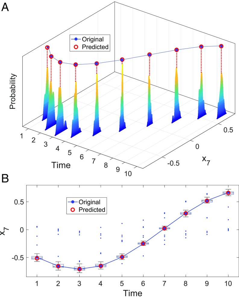
To illustrate the mechanism and the basic idea of the RDE framework, we begin with a benchmark model with additive noise. The model contains 10 interacted variables, showing dynamical behavior of attractive periodicity that has a box-counting dimension that is $d=1$ in the 10D space (the details of the system are provided in SI Appendix). According to the RDE framework, multiple tuples of two components could be randomly chosen and used to make one-step prediction for the underlined component $x_7$. In the noise-free situation, the majority of the randomly chosen index tuples (the 2D random embeddings) can bring accurate prediction, while there are some degenerative cases where the chosen index tuple cannot make good prediction, yielding large errors. Fig. 2A shows the numerical results of one-step prediction under the noise-free condition, where the distribution of the prediction errors presents a delta function-like form at the zero error, leaving small probability of large errors. In the situation where the time series data are deteriorated by noise, each embedding shows different ability to cope with noise when making prediction due to the different way in which the random embedding preserves the dynamical information of the entire system. Accordingly, the distribution of the prediction errors shows a normal distribution-like form except for the outliers in the degenerative cases as shown in Fig. 2B. In Fig. 2C, the distribution is further dispersed under a higher level of noise strength while keeping the distribution center at zero. The prediction of the benchmark system under noise deterioration using the RDE framework is further carried out in Fig. 4, where the distribution of the prediction and the final predicted value as well as outliers are depicted for each one-step prediction. The correlation between the predicted values and the real values reaches 0.99, confirming that the RDE framework works effectively in accurate prediction for the benchmark model, even under noise deterioration.

Fig. 4.

Ten time points of one-step prediction for one variable in the benchmark model of a linear system. (A) The distribution of prediction by random embeddings. Based on this information, the final predicted values are made. (B) In addition to the original data and the predicted data, the box plot of the distribution is also shown in plane with median values, upper and lower quartiles, bounds, and outliers.

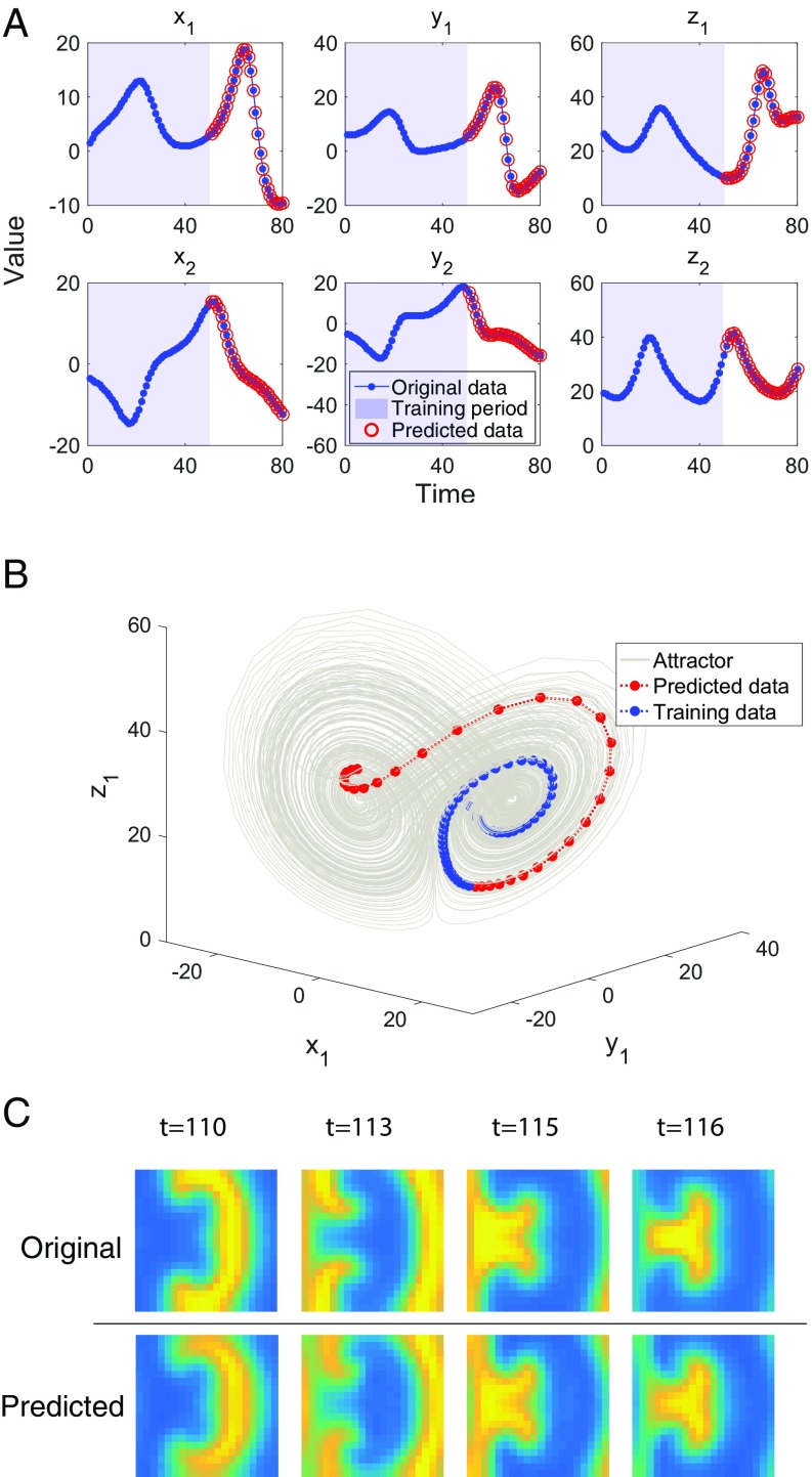
To validate the applicability of the RDE framework to make multistep prediction for high-dimensional nonlinear systems, we consider a 90D coupled Lorenz system. As shown in Fig. 5 A and B, the multistep dynamics of the 90D system can be accurately predicted from a measured time series with only 50 time points, which clearly covers small segments of the attractor.

Fig. 5.

Validations with synthetic data. (A) Prediction for the nonlinear 90D coupled Lorenz system, where multistep prediction up to 30 steps for six components is shown. (B) For the coupled Lorenz system of 90 dimensions, the training data as well as the predicted data cover only small segments of the underlying attractor. Each circle represents a data point corresponding to the data in A; some data points are buried within the attractor. (C) Prediction for $20\times 20$ grids of a spiral pattern in an ISCAM model, where four selective samples of one-step prediction for the pattern are shown.

Spatiotemporal dynamics produces data evolving across time as well as space (43, 44), such as one of the typical high-dimensional systems involving a large number of interacted variables. Since the variables interact with each other in an unknown manner, the prediction of such a multivariable system based on limited time series data thus becomes a challenging task. We consider the data generated from an ideal storage cellular automaton model (ISCAM) simulating heterocatalytic reaction–diffusion processes at metal surfaces (45, 46). The one-step prediction results by using the RDE framework for a spiral pattern in the $20\times 20$ grids are illustrated in Fig. 5C, which clearly shows the effectiveness of our method for the spatiotemporal pattern prediction. Here, 800 variables are involved in the system, and 100 consecutive pattern series are observed as the training set.

Real-World Data.

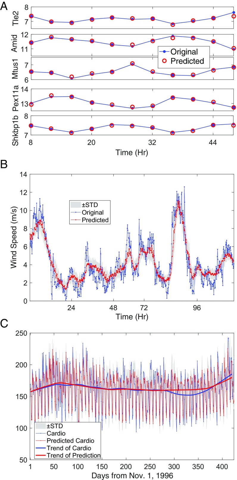
In the era of big-data, high-dimensional data are ubiquitously collected from numerous real-world systems. We first consider a set of gene expression data as representative high-throughput biological data, typically with a large number of genes but with a very small number of time sampling points. The dataset was obtained by a gene expression profiling study of both miRNA and mRNA in mouse liver (47), which consists of time series containing 12 time points of 46,628 probes (each probe measures every 4 h over 48 h). Due to the complicated gene regulation mechanism (48), despite the high dimension and different types of probes or genes, the time evolution of all of these probes can be regulated by certain underlying complicated regulation dynamics, thus forming a high-dimensional dynamical system. Consequently, it is possible to use the RDE framework to predict the gene expression dynamics of each specific probe. As shown in Fig. 6A, the RDE framework achieves fairly accurate one-step prediction in a leave-one-out way.

Fig. 6.

Real-world data. (A) One-step prediction for five probes from the gene dataset. (B) A 1-h prediction for the wind speed in the Tokyo capital region based on data collected from five geometrically local stations and delays up to 5 h. (C) A 1-d prediction for the daily cardiovascular disease admissions with trend, where the standard deviation (STD) is shown as shaded area.

Climate datasets, usually collected at different locations by regular sampling intervals, are known by their complex spatiotemporal characteristics. Here, we consider the wind speed datasets collected around the Tokyo capital region in Japan by the Japan Meteorological Agency (49). Taking delays for each factor into consideration, the system shows a high-dimensional property, and the 1-h prediction is made by the RDE framework with a training set containing 400 time points as shown in Fig. 6B. The correlation between the predicted series and the original series reaches 0.9.

The final real data test comes from the city of Hong Kong, and it is composed of time series of air pollutants and disease admissions in major hospitals in Hong Kong (50, 51). Considering the delay effect of every potential factor as well as a dummy vector of weekday effect (52), we have a 48D system, and without the RDE framework, it is difficult to predict the disease admissions with only 200 observations in high accuracy. However, by using the RDE framework, the 1-d forward prediction is obtained as shown in Fig. 6C, where the correlation between the predicted values and the original values reaches 0.74 and the predicted trend of the disease risk fits fairly well with the true trend.

Discussion

Expectation Scheme or Aggregation Scheme.

The expectation scheme is simple and straightforward for applications. However, the aggregation scheme needs fitting error estimation before making final prediction. Considering the short-term property of the training set, we adopt a leave-one-out strategy to obtain the fitting error for the aggregation scheme. Thus, the aggregation scheme requires higher computational cost than the expectation scheme, but it does not rely on the zero-mean assumption of the prediction errors as summarized in SI Appendix. Notice that the distribution of such a prediction error is unknown a priori. Then, it is nontrivial to make a selection from these two schemes in advance. For the choice, we judge whether or not the distribution of prediction is symmetric using the skewness quantity for a distribution. Larger skewness suggests that the distribution is asymmetric and consequently, that the normal expectation is unlikely to become the best candidate for the final prediction. The effectiveness of the skewness is further illustrated by using a benchmark system as shown in SI Appendix.

Number of Mappings from Nondelay Attractors to a Delay Attractor.

The advantage of the RDE framework exists in decoding the intertwined information among various variables of a complex system by considering a large number of embeddings in low-dimensional subspaces. Specifically, the number of possible nondelay embeddings grows combinatorially as the system dimension increases in a manner as

$$m=\left(\begin{array}{c}n\hfill \\ L\hfill \end{array}\right),$$

where $n$ is the number of observed variables and $L$ is the embedding dimension. However, if we intend to obtain all of the possible nondelay embeddings as $n$ increases, the computational cost grows drastically, and the curse of dimensionality problem emerges unavoidably. As a matter of fact, in practice it is neither necessary nor practically profitable to exhaust all of the candidate nondelay embeddings. When we estimate the expectation of the underlined distribution, according to the sampling theory (53, 54), the width of the confidence interval for the estimated expectation decreases as the number of sampling increases. Particularly for the normal distribution, the confidence interval could even be analytically provided in advance (SI Appendix). With this interval, only a small number of random embeddings are sufficient to reach the precision of the expectation estimation scheme. Actually, the computation of all of the corresponding mappings is highly parallel, and thus, the computational cost can be further alleviated by using parallel computation. For the aggregation scheme, however, we use the in-sample test or the Monte Carlo method with replacement to score candidate random embeddings. In fact, as the number of random embeddings increases, the best in-sample error (or the fitting error) decreases exponentially as shown in SI Appendix. Thus, we terminate random embeddings sampling when the in-sample error converges (at the elbow of the exponential decrease), which reduces computational cost and brings good generalization as well.

Short-Term Data, Robustness, and Comparisons.

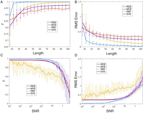
Since the RDE framework fully exploits the information embedded in low-dimensional attractors and does not require the coverage of the whole attractor, it is possible to deal with very limited training data. To validate this, we carry out a length test on the coupled Lorenz systems with 15 variables. The test is based on multiple randomly selected sections of measured data. The results are shown in Fig. 7 A and B, where two criteria for one-step predictions are plotted vs. the length of measured data. Compared with other prediction methods for high-dimensional data, the RDE framework particularly works well with very short-term data. Clearly, around 20 time points of the measured data are sufficient for reconstructing system’s dynamics. In the literature, both the classic single-variable embedding (SVE) method (11) and the recently proposed multiview embedding (MVE) method (55) can deal with the prediction of high-dimensional data. To make predictions, they both rely on the nearest neighbors in the attractor reconstructed by the historical data, and thus, they may suffer from false nearest neighbors when the length of the time series data is very short. However, the RDE framework does not require that the measured data (training data) cover the whole attractor. It works effectively even when only small segments of the attractor are covered by the measured data as shown in Fig. 5B. As clearly shown in Fig. 7 A and B, for the same short-term data (less than 30 points), both methods, MVE and SVE, have poor convergence, while the RDE framework performs well. Indeed, MVE and SVE work well only when the training data become longer (but they are still far from convergence), since longer training data produce better coverage of the nearest neighbors in the attractor.

Fig. 7.

Performance comparisons of different methods with different lengths of training data and different levels of noise. Two criteria are used to evaluate the prediction quality: the correlation $\rho$ and the rms error between the predicted series and the test data. (A and B) The length test based on 100 randomly chosen sections for each length of training data. (C and D) The noise test based on 100 independent trials. Here, the median, the upper quartile, and the lower quartile are shown. SNR, signal-to-noise ratio.

Noise is inevitable in real applications, and to test the practical robustness of the RDE framework, we also consider the effect of additive white noise in the above 15D coupled Lorenz system with 50 time points as training data. Fig. 7 C and D shows that the RDE framework works well for the signal-to-noise ratio larger than 10, which is as robust as the empirical data-based MVE and SVE methods. Moreover, although both the RDE framework and the RBF (radial basis function) network method proposed in ref. 33 use the inverse embedding technique, the RDE framework fully leverages the information in the distribution of a large amount of random embeddings, while the RBF method uses inverse embedding directly for a high-dimensional system. This difference outstandingly promotes the robustness of the RDE framework against noise deterioration as shown in Fig. 7 C and D.

Conclusion

In summary, we have established a framework to make predictions from short-term high-dimensional data accurately. The novelty of this RDE framework roots in a full exploitation of the information embedded in a large number of low-dimensional nondelay attractors as well as in an appropriate use of the exploited distribution of the target variable for prediction. On one hand, the RDE framework creates a distribution, patching all pieces of information from various embeddings into the entire dynamics of the predicted variable. On the other hand, the selection of suitable estimation schemes based on the distribution information thereby significantly increases the prediction reliability and robustness, even for those short-term data with noise deterioration. As validated by datasets produced by both benchmark models and real-world systems, the method is especially effective for the observed short-term high-dimensional time series. This virtue makes the RDE framework potentially useful in mining big datasets from real-world systems.

Materials and Methods

Given time series data sampled from $n$ variables of a system with length $m$ (i.e., $\mathbf{x}\left(t\right)\in {\mathbb{R}}^n,t=t_1,t_2,\dots ,t_m$, where $t_i=t_{i-1}+\tau$), one can estimate the box-counting dimension $d$ of the system’s dynamics using the false nearest neighbor algorithm (56) and choose embedding dimension $L>2d$. Assume that the target variable to be predicted is represented as $x_k$. The RDE algorithm is listed as follows:

• ∙Randomly pick $s$ tuples from $\left(\mathrm{1,2},\dots ,n\right)$ with replacement, and each tuple contains $L$ numbers.
• ∙For the $l$th tuple $\left(l_1,l_2,\dots ,l_L\right)$, fit a predictor ${\psi }_l$ so as to minimize ${\sum }_{i=1}^{m-1}\Vert x_k\left(t_i+\tau \right)-{\psi }_l\left(x_{l_1}\left(t_i\right),x_{l_2}\left(t_i\right),\dots ,x_{l_L}\left(t_i\right)\right)\Vert$. Standard fitting algorithms could be adopted. In this paper, Gaussian Process Regression is used.
• ∙Use each predictor ${\psi }_l$, and make one-step prediction ${\tilde{x}}_k^l\left(t*+\tau \right)={\psi }_l\left(x_{l_1}\left(t*\right),x_{l_2}\left(t*\right),\dots ,x_{l_L}\left(t*\right)\right)$ for a specific future time $t*+\tau$.
• ∙Multiple predicted values form a set $\left\{{\tilde{x}}_k^l\left(t*+\tau \right)\right\}$. Exclude the outliers from the set, and use the Kernel Density Estimation method to approximate the probability density function $p\left(x\right)$ of its distribution.
• ∙Calculate the skewness $\gamma$ of such distribution. In the case $\gamma <\xi$, where $\xi$ is a threshold value, make the final prediction as ${\tilde{x}}_k\left(t*+\tau \right)=\int xp\left(x\right)\mathrm{d}x$. Otherwise, calculate the in-sample prediction error ${\delta }_l$ for the fitted ${\psi }_l$ using the leave-one-out method. Based on the rank of the in-sample error, $r$ best tuples are picked out, and the final prediction is given by the aggregated average in the form of ${\tilde{x}}_k\left(t*+\tau \right)=\sum _{i=1}^r{\omega }_i{\tilde{x}}_k^{l_i}\left(t*+\tau \right)$, where the weight ${\omega }_i=\frac{\exp \left(-{\delta }_i/{\delta }_1\right)}{{\sum }_j\exp \left(-{\delta }_j/{\delta }_1\right)}$.

Here, the condition $\gamma <\xi$ implies that the distribution is nearly symmetric; then, the expectation of the distribution is used as the final prediction. Otherwise, the distribution is asymmetric, indicating that the expectation is not the best choice for the final prediction; then, the aggregation average is used as the final prediction. In this work, we empirically set $\xi$ as 0.1, and a statistical hypothesis test with shuffling data could be carried out to get a significant level. In this algorithm, the number $s$ of tuples is determined using a confidence interval or convergence of in-sample errors as given in SI Appendix, and the number $r$ of best tuples is empirically chosen as $L$. The RDE algorithm described above is for one-step prediction, but the RDE framework can be extended to multistep prediction. Particularly for the case where ${\psi }_l$ is approximated as a linear mapping, the form of ${\psi }_l$ can be further explicitly obtained as presented in SI Appendix.

References

- 1.Lockhart DJ, Winzeler EA. Genomics, gene expression and DNA arrays. Nature. 2000;405:827–836. doi: 10.1038/35015701. [DOI] [PubMed] [Google Scholar]
- 2.De Jong H. Modeling and simulation of genetic regulatory systems: A literature review. J Comput Biol. 2002;9:67–103. doi: 10.1089/10665270252833208. [DOI] [PubMed] [Google Scholar]
- 3.Stein RR, et al. Ecological modeling from time-series inference: Insight into dynamics and stability of intestinal microbiota. PLoS Comput Biol. 2013;9:e1003388. doi: 10.1371/journal.pcbi.1003388. [DOI] [PMC free article] [PubMed] [Google Scholar]
- 4.Rienecker MM, et al. Merra: NASA’s modern-era retrospective analysis for research and applications. J Clim. 2011;24:3624–3648. doi: 10.1175/JCLI-D-16-0758.1. [DOI] [PMC free article] [PubMed] [Google Scholar]
- 5.Fan J, Han F, Liu H. Challenges of big data analysis. Natl Sci Rev. 2014;1:293–314. doi: 10.1093/nsr/nwt032. [DOI] [PMC free article] [PubMed] [Google Scholar]
- 6.Clauset A, Larremore DB, Sinatra R. Data-driven predictions in the science of science. Science. 2017;355:477–480. doi: 10.1126/science.aal4217. [DOI] [PubMed] [Google Scholar]
- 7.Subrahmanian V, Kumar S. Predicting human behavior: The next frontiers. Science. 2017;355:489–489. doi: 10.1126/science.aam7032. [DOI] [PubMed] [Google Scholar]
- 8.Hamilton JD. Time Series Analysis. Vol 2 Princeton Univ Press; Princeton: 1994. [Google Scholar]
- 9.Ma H, Lin W. Realization of parameters identification in only locally lipschitzian dynamical systems with multiple types of time delays. SIAM J Control Optim. 2013;51:3692–3721. [Google Scholar]
- 10.Ma H, Lin W. Nonlinear adaptive synchronization rule for identification of a large amount of parameters in dynamical models. Phys Lett A. 2009;374:161–168. [Google Scholar]
- 11.Farmer JD, Sidorowich JJ. Predicting chaotic time series. Phys Rev Lett. 1987;59:845–848. doi: 10.1103/PhysRevLett.59.845. [DOI] [PubMed] [Google Scholar]
- 12.Wang WX, Lai YC, Grebogi C. Data based identification and prediction of nonlinear and complex dynamical systems. Phys Rep. 2016;644:1–76. [Google Scholar]
- 13.Hinton GE, Osindero S, Teh YW. A fast learning algorithm for deep belief nets. Neural Comput. 2006;18:1527–1554. doi: 10.1162/neco.2006.18.7.1527. [DOI] [PubMed] [Google Scholar]
- 14.Hochreiter S, Schmidhuber J. Long short-term memory. Neural Comput. 1997;9:1735–1780. doi: 10.1162/neco.1997.9.8.1735. [DOI] [PubMed] [Google Scholar]
- 15.Jaeger H. 2001. The “echo state” approach to analysing and training recurrent neural networks (German National Research Center for Information Technology GMD, Bonn), Technical Report 148(34):13.
- 16.Maass W, Natschläger T, Markram H. Real-time computing without stable states: A new framework for neural computation based on perturbations. Neural Comput. 2002;14:2531–2560. doi: 10.1162/089976602760407955. [DOI] [PubMed] [Google Scholar]
- 17.Jaeger H, Haas H. Harnessing nonlinearity: Predicting chaotic systems and saving energy in wireless communication. Science. 2004;304:78–80. doi: 10.1126/science.1091277. [DOI] [PubMed] [Google Scholar]
- 18.Pathak J, Hunt B, Girvan M, Lu Z, Ott E. Model-free prediction of large spatiotemporally chaotic systems from data: A reservoir computing approach. Phys Rev Lett. 2018;120:024102. doi: 10.1103/PhysRevLett.120.024102. [DOI] [PubMed] [Google Scholar]
- 19.Ma H, Lin W, Lai YC. Detecting unstable periodic orbits in high-dimensional chaotic systems from time series: Reconstruction meeting with adaptation. Phys Rev E. 2013;87:050901. doi: 10.1103/PhysRevE.87.050901. [DOI] [PubMed] [Google Scholar]
- 20.Kuremoto T, Kimura S, Kobayashi K, Obayashi M. Time series forecasting using a deep belief network with restricted Boltzmann machines. Neurocomputing. 2014;137:47–56. [Google Scholar]
- 21.Xingjian S, et al. Convolutional lstm network: A machine learning approach for precipitation nowcasting. In: Cortes C, Lawrence ND, Lee DD, Sugiyama M, Garnett R, editors. Advances in Neural Information Processing Systems. Curran Associates, Inc.; Montreal: 2015. pp. 802–810. [Google Scholar]
- 22.Lu Z, et al. Reservoir observers: Model-free inference of unmeasured variables in chaotic systems. Chaos Interdiscip J Nonlinear Sci. 2017;27:041102. doi: 10.1063/1.4979665. [DOI] [PubMed] [Google Scholar]
- 23.Pathak J, Lu Z, Hunt BR, Girvan M, Ott E. Using machine learning to replicate chaotic attractors and calculate Lyapunov exponents from data. Chaos Interdiscip J Nonlinear Sci. 2017;27:121102. doi: 10.1063/1.5010300. [DOI] [PubMed] [Google Scholar]
- 24.Larger L, et al. High-speed photonic reservoir computing using a time-delay-based architecture: Million words per second classification. Phys Rev X. 2017;7:011015. [Google Scholar]
- 25.Yeo K, Melnyk I. 2018. Deep learning algorithm for data-driven simulation of noisy dynamical system. arXiv:1802.08323.
- 26.Pathak J, et al. Hybrid forecasting of chaotic processes: Using machine learning in conjunction with a knowledge-based model. Chaos Interdiscip J Nonlinear Sci. 2018;28:041101. doi: 10.1063/1.5028373. [DOI] [PubMed] [Google Scholar]
- 27.Haykin S. Neural Networks: A Comprehensive Foundation. Macmilan; New York: 1994. [Google Scholar]
- 28.Dambre J, Verstraeten D, Schrauwen B, Massar S. Information processing capacity of dynamical systems. Sci Rep. 2012;2:514. doi: 10.1038/srep00514. [DOI] [PMC free article] [PubMed] [Google Scholar]
- 29.Pearson K. On lines and planes of closest fit to systems of points in space. Lond Edinb Dublin Philos Mag J Sci. 1901;2:559–572. [Google Scholar]
- 30.Hotelling H. Analysis of a complex of statistical variables into principal components. J Educ Psychol. 1933;24:417–441. [Google Scholar]
- 31.Tibshirani R. Regression shrinkage and selection via the lasso. J R Stat Soc Ser B. 1996;73:273–282. [Google Scholar]
- 32.Candes EJ, Romberg JK, Tao T. Stable signal recovery from incomplete and inaccurate measurements. Commun Pure Appl Math. 2006;59:1207–1223. [Google Scholar]
- 33.Ma H, Zhou T, Aihara K, Chen L. Predicting time series from short-term high-dimensional data. Int J Bifurcation Chaos. 2014;24:1430033. [Google Scholar]
- 34.Van Der Maaten L, Postma E, Van den Herik J. Dimensionality reduction: A comparative. J Mach Learn Res. 2009;10:66–71. [Google Scholar]
- 35.Kantz H, Schreiber T. Nonlinear Time Series Analysis. Vol 7 Cambridge Univ Press; Cambridge, UK: 2004. [Google Scholar]
- 36.Takens F. Detecting strange attractors in turbulence. In: Rand DA, Young L-S, editors. Dynamical Systems and Turbulence, Warwick 1980. Springer; Berlin: 1981. pp. 366–381. [Google Scholar]
- 37.Sauer T, Yorke JA, Casdagli M. Embedology. J Stat Phys. 1991;65:579–616. [Google Scholar]
- 38.Packard NH, Crutchfield JP, Farmer JD, Shaw RS. Geometry from a time series. Phys Rev Lett. 1980;45:712–716. [Google Scholar]
- 39.Deyle ER, Sugihara G. Generalized theorems for nonlinear state space reconstruction. PLoS One. 2011;6:e18295. doi: 10.1371/journal.pone.0018295. [DOI] [PMC free article] [PubMed] [Google Scholar]
- 40.Rasmussen C, Williams C. Gaussian Processes for Machine Learning. MIT Press; Cambridge, MA: 2006. [Google Scholar]
- 41.Ho TK. The random subspace method for constructing decision forests. IEEE Trans Pattern Anal Mach Intell. 1998;20:832–844. [Google Scholar]
- 42.Bryll R, Gutierrez-Osuna R, Quek F. Attribute bagging: Improving accuracy of classifier ensembles by using random feature subsets. Pattern Recognit. 2003;36:1291–1302. [Google Scholar]
- 43.Colizza V, Pastor-Satorras R, Vespignani A. Reaction–diffusion processes and metapopulation models in heterogeneous networks. Nat Phys. 2007;3:276–282. [Google Scholar]
- 44.Kondo S, Miura T. Reaction-diffusion model as a framework for understanding biological pattern formation. Science. 2010;329:1616–1620. doi: 10.1126/science.1179047. [DOI] [PubMed] [Google Scholar]
- 45.Dress A, Hordijk W, Lin W, Serocka P. 2010. The ideal storage cellular automaton model. Structure Discovery in Biology: Motifs, Networks & Phylogenies, Dagstuhl Seminar Proceedings, eds Apostolico A, Dress A, Parida L (Schloss Dagstuhl - Leibniz-Zentrum fuer Informatik, Dagstuhl, Germany), pp 1862–4405.
- 46.Dress AW, Lin W. Dynamics of a discrete-time model of an“ideal-storage” system describing hetero-catalytic processes on metal surfaces. Int J Bifurcation Chaos. 2011;21:1331–1339. [Google Scholar]
- 47.Na YJ, et al. Comprehensive analysis of microrna-mrna co-expression in circadian rhythm. Exp Mol Med. 2009;41:638–647. doi: 10.3858/emm.2009.41.9.070. [DOI] [PMC free article] [PubMed] [Google Scholar]
- 48.Shen-Orr SS, Milo R, Mangan S, Alon U. Network motifs in the transcriptional regulation network of Escherichia coli. Nat Genet. 2002;31:64–68. doi: 10.1038/ng881. [DOI] [PubMed] [Google Scholar]
- 49.Hirata Y, Aihara K. Predicting ramps by integrating different sorts of information. Eur Phys J Spec Top. 2016;225:513–525. [Google Scholar]
- 50.Wong TW, et al. Air pollution and hospital admissions for respiratory and cardiovascular diseases in Hong Kong. Occup Environ Med. 1999;56:679–683. doi: 10.1136/oem.56.10.679. [DOI] [PMC free article] [PubMed] [Google Scholar]
- 51.Fan J, Zhang W. Statistical estimation in varying coefficient models. Ann Stat. 1999;27:1491–1518. [Google Scholar]
- 52.Xia Y, Härdle W. Semi-parametric estimation of partially linear single-index models. J Multivar Anal. 2006;97:1162–1184. [Google Scholar]
- 53.Kish L. Survey Sampling. John Wiley & Sons; New York: 1995. [Google Scholar]
- 54.Hogg RV, Craig AT. Introduction to Mathematical Statistics. 5th Ed Prentice Hall; Upper Saddle River, NJ: 1995. [Google Scholar]
- 55.Ye H, Sugihara G. Information leverage in interconnected ecosystems: Overcoming the curse of dimensionality. Science. 2016;353:922–925. doi: 10.1126/science.aag0863. [DOI] [PubMed] [Google Scholar]
- 56.Kennel MB, Brown R, Abarbanel HDI. Determining embedding dimension for phase-space reconstruction using a geometrical construction. Phys Rev A. 1992;45:3403–3411. doi: 10.1103/physreva.45.3403. [DOI] [PubMed] [Google Scholar]
Associated Data
This section collects any data citations, data availability statements, or supplementary materials included in this article.