Modeling Brain Dynamic State Changes with Adaptive Mixture Independent Component Analysis

Modeling Brain Dynamic State Changes with Adaptive Mixture Independent Component Analysis

There is a growing interest in neuroscience in assessing the continuous, endogenous, and nonstationary dynamics of brain network activity supporting the fluidity of human cognition and behavior. This non-stationarity may involve ever-changing formation and dissolution of active cortical sources and brain networks. However, unsupervised approaches to identify and model these changes in brain dynamics as continuous transitions between quasi-stable brain states using unlabeled, noninvasive recordings of brain activity have been limited. This study explores the use of adaptive mixture independent component analysis (AMICA) to model multichannel electroencephalographic (EEG) data with a set of ICA models, each of which decomposes an adaptively learned portion of the data into statistically independent sources. We first show that AMICA can segment simulated quasi-stationary EEG data and accurately identify ground-truth sources and source model transitions. Next, we demonstrate that AMICA decomposition, applied to 6–13 channel scalp recordings from the CAP Sleep Database, can characterize sleep stage dynamics, allowing 75% accuracy in identifying transitions between six sleep stages without use of EEG power spectra. Finally, applied to 30-channel data from subjects in a driving simulator, AMICA identifies models that account for EEG during faster and slower response to driving challenges, respectively. We show changes in relative probabilities of these models allow effective prediction of subject response speed and moment-by-moment characterization of state changes within single trials. AMICA thus provides a generic unsupervised approach to identifying and modeling changes in EEG dynamics. Applied to continuous, unlabeled multichannel data, AMICA may likely be used to detect and study any changes in cognitive states.

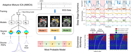
Graphical Abstract

1. Introduction

An expanding focus in neuroscience has been on endogenous temporal dynamics of neural network activity that gives rise to fluidity and rapid adaptability in cognition and behavior. A growing body of evidence suggests that these temporal dynamics may arise from continual formation and dissolution of interacting cortical and allied subcortical source activities in large-scale brain regions whose joint electrical activities can be described as dynamic systems featuring continuous transitions between intermittently stable states (Chu et al., 2012; Betzel et al., 2012). The temporal dynamics and network topology of these “brain states” can be identified using functional neuroimaging techniques including invasive electrophysiological recordings, functional MRI (fMRI), magnetoencephalography (MEG), and electroencephalography (EEG) (Freyer et al., 2009; Chu et al., 2012). Among noninvasive modalities, EEG provides a more direct measurement of brain activity with millisecond resolution that, because of the low weight and bulk of its sensors, is appropriate for studying fast-changing brain states in real-world environments.

Earlier methods applied nonparametric statistical approaches that used EEG power spectral density, autocorrelation function, and entropy measures (Natarajan et al., 2004) to detect change points allowing segmentation of EEG into piecewise stationary processes (Kaplan et al., 2001). Microstate analysis (see Khanna et al. (2015) for a review) takes the spatial distribution of electrodes into account and attempts to define quasi-stable “microstates” in terms of unique electric potential patterns across the multichannel EEG scalp electrode montage during behavioral states or resting states (Lehmann et al., 1987; Van de Ville et al., 2010). The global functional connectivity approach (Chu et al., 2012; Betzel et al., 2012) measures inter-electrode channel signal synchrony to attempt to characterize brain states as stable functional networks. However, both the microstate and global connectivity models analyze scalp electrode signals that in themselves are highly correlated through common volume conduction and summation at the electrodes of potentials arising from brain and also non-brain sources (eye movements, ECG, etc.). The results of both methods have few or no interpretable connections to particular brain source activities that underlie the observed scalp phenomena. Hidden Markov Models (HMM) form another family of generative models with a rigorous temporal structure used to measure nonstationary functional connectivity. Such models have been largely applied to source-space signals from MEG recordings (Baker et al., 2014; Vidaurre et al., 2016, 2017; Nielsen et al., 2017), where a source separation or localization step is prerequisite.

To study source-resolved EEG activities, independent component analysis (ICA) (Jutten and Herault, 1991; Bell and Sejnowski, 1995) has been widely applied as a means for blind source separation (Makeig et al., 1996; Jung et al., 2000; Makeig et al., 2002). ICA models data, x, as an instantaneous linear mixture of statistically independent source processes, s (x = A·s, where A is a mixing matrix). A physiological interpretation of ICA applied to scalp EEG recordings can be found in Onton et al. (2006) and Delorme et al. (2012). In short, this research has clarified: 1) functional independence across brain regions, similar to the regional dependence and independence now measured by functional brain mapping using fMRI, should be accompanied by temporal independence of the source EEG activities; 2) linear and instantaneous mixing of source EEG activities is produced by volume conduction and scalp mixing. While ICA works well in separating out localized cortical sources of event-related potentials and eye-movement related activity, it is limited in modeling nonstationary changes in EEG source locations and activities because of its spatial-stationarity assumption produced by its limited model complexity (e.g., its use of a fixed spatial mixing matrix in which the number of learned temporally independent components is equal to the number of channels measured).

Our recent study (Hsu and Jung, 2017) hypothesized that transitions to a different cognitive state may involve cortical macro- or meso-dynamics in new networks of cortical brain areas that can be identified by distinct ICA models trained on data recorded before and after the state transition, respectively. This hypothesis motivates the application of an extension of ICA – the ICA mixture model (ICAMM) (Lee et al., 2000) – an unsupervised learning approach to modeling EEG activities in different brain states and detecting brain dynamic state changes associated with cognitive state changes (Jung et al., 2000). The ICAMM assumes distinct ICA models may better characterize different segments of nonstationary data, i.e., x(t) = A_hs_h(t) where h is the model index. By allowing multiple ICA models to focus simultaneously on different parts of the data, ICAMM relaxes the spatial-stationarity assumptions and allows more total sources to be learned than the number of channels. ICAMM is thereby capable of modeling nonstationary, multi-state data and thus is a promising approach to studying dynamic changes in cognition and brain states. While the few prior attempts to apply ICAMM to EEG data were able to monitor attention (Jung et al., 2000), to detect microarousals during sleep (Salazar et al., 2010a), and to detect mental state changes during a memory test (Safont et al., 2017), the full power of the ICAMM approach has not yet been demonstrated, including modeling of multiple brain states, tracking of state transitions in continuous recordings, consistency of the learned models across subjects, and more precise physiological interpretation of those models.

Here we report an EEG study using an unsupervised ICAMM to investigate dynamics of cognitive states. For this we chose an adaptive mixture ICA (AMICA), proposed by Palmer et al. (2008) that adaptively learns individual source probability density functions (PDFs) as well as source scalp projection patterns. Palmer et al. (2008) has also provided an efficiently optimized algorithm for learning an ICAMM from multichannel data using a parallel implementation (the code is available at https://sccn.ucsd.edu/~jason/amica_web.html and also as an open source plug-in for EEGLAB (Delorme and Makeig, 2004) at https://sccn.ucsd.edu/wiki/EEGLAB_Extensions_and_plug-ins). In the following sections, we will show: 1) AMICA can learn the ground truth in the simulated quasi-stationary data – we test the effect of numbers of ICA models on AMICA performance; 2) AMICA usefully characterizes sleep EEG dynamics, producing consistent results across subjects that can be applied to classify six sleep stages; 3) AMICA can quantitatively assess subjects’ continuous changes in attention and drowsiness levels during simulated driving and thereby can track brain dynamic state changes at single-trial level with millisecond resolution; and 4) AMICA provides interpretable models allowing computation of the spatial distribution and frequency content of active sources in each brain state.

2. Materials and Methods

2.1. Datasets and preprocessing

2.1.1. Dataset I: simulated quasi-stationary data

To systematically validate AMICA, we use the EEG data simulator in the Source Information Flow Toolbox (SIFT) (Delorme et al., 2011) to simulate a quasi-stationary dataset in which underlying sources are alternatingly active and inactive. With a 3-layer boundary-element-method (BEM) forward model, we obtain three 3-min segments of simulated 16-channel EEG data, each with a different set of 16 active super-Gaussian distributed sources. More details are included in Supplementary Materials (Section 1) and in Hsu et al. (2015).

2.1.2. Dataset II: CAP sleep database

We used 17 human EEG recordings, each consisting of 6–10 hours of sleep, from the CAP sleep database (Terzano et al., 2002) on PhysioNet (Goldberger et al., 2000). Excluding subjects whose recordings had less than 5 channels gave 7 EEG datasets from healthy subjects. We also used EEG recordings from 10 patients with nocturnal frontal lobe epilepsy (NFLE), selected on the basis of data quality, i.e., longer data length, higher number of channels and more balanced numbers of sleep labels. We included NFLE patient recordings in an attempt to test the ability of the proposed approach to generalize across subjects and patients.

The EEG data comprise 6–13 bipolar channels (e.g., F3–C3, C3–P3, P3–O1, O1–A1, without common reference) a xed at scalp sites in the International 10–20 System and recorded with a sampling rate of 128 Hz using a Galileo System (Esaote Biomedica). After collection, the EEG signals were band-pass filtered between 0.5 Hz to 25 Hz. The hypnograms had been annotated by expert neurologists at 30-second intervals using standard Rechtscha en and Kales (R&K) criteria into 6 sleep stages: wake (W), rapid eye movement (REM), and 1 to 4 non-REM sleep stages (N1, N2, N3 and N4). More detailed description of the data and their hypnograms can be found at https://physionet.org/pn6/capslpdb/.

2.1.3. Dataset III: drowsiness fluctuation in simulated driving

Ten healthy volunteers participated in a 90-min experiment in an immersive VR-based driving simulator, performing an event-related lane-departure task (Huang et al., 2009). The subjects experienced visually presented lane-departure events every 8–12 seconds (with randomized event onset asynchronies) and were instructed to steer the car back to the cruising position quickly using a steering wheel. The duration between the onset of a lane-departure event to the onset of a responsive steering action was defined as subject reaction time (RT), which can be used to index degree of subject alertness / drowsiness (Lin et al., 2010). The RT data were transformed to reaction speed (RS = 1/RT) to partially normalize the highly skewed RT distribution. For more details on the subjects and the experiment, refer to Lin et al. (2010).

For each subject, 30-channel EEG data were recorded with a 500-Hz sampling rate using a NeuroScan System (Compumedics Ltd., VIC, Australia) with electrode sites according to the International 10–20 System. The EEG data were band-pass filtered (1–50 Hz) and downsampled to 250 Hz. Using the PREP pipeline (Bigdely-Shamlo et al., 2015), poorly recorded channels in the recordings, such as channels with flat signals arising from poor electrode contacts, and channels whose signals were poorly correlated with those of neighboring channels were removed. Two to six channels were so identified and removed for each of the 10 subjects. In addition, artifact subspace reconstruction (ASR) (Mullen et al., 2015), implemented as a plug-in to the EEGLAB environment (Delorme and Makeig, 2004), was applied using a mild threshold (burst repair σ = 20) to reduce data contamination by high-amplitude artifacts. These artifact-correction methods were chosen to facilitate convergence of the ICA models. Detailed description of the data pre-processing can be found in Hsu and Jung (2017).

2.2. Method description

Comprehensive formulation of the ICAMM problem and detailed derivation of the AMICA algorithm have been presented in Lee et al. (2000) and Palmer et al. (2008) respectively. The following sections give a brief summary of the multi-model AMICA approach in an attempt to provide intuition and facilitate readers’ understanding.

2.2.1. Adaptive mixture ICA (AMICA)

Fig. 1 gives a schematic overview of the architecture of AM ICA and its models. AMICA is, conceptually, a three-layer mixing network: the top two layers constitute one or more ICA mixture models and the bottom layer, specific to AMICA, focuses each learned model on accounting for a subset of the data.

Figure 1:

Adaptive Mixture ICA (AMICA) in a nutshell. AMICA consists of three layers of mixing. As shown in illustration, the first layer is mixture of ICA models A₁ and A₂ that learn the underlying data clusters, simulated based on Laplace and uniform distribution respectively. The second layer is mixture of independent components A₁₁ and A₁₂ that decompose the data cluster into statistically independent sources’ activations s₁₁ and s₁₂. The third layer is mixture of generalized Gaussian distributions q_11j that approximate the probability distribution of the source activation p(s₁₁).

Starting from the top layer, the key assumption of multiple mixture models is that data X = {x(t)} (N-channel by T-time samples) are nonstationary, so that different models may be dominant in characterizing the data at different times, i.e., x(t) = x_h(t) where h is the model index. Previous studies have provided evidence that EEG activities during different brain states (e.g., alert versus drowsy) are nonstationary and can be modeled by a finite set of distinct ICA models (Hsu and Jung, 2017).

In the top two layers of the AMICA network, a standard ICA model is employed to model the data x as an instantaneous linear mixture A (N × N matrix) of statistically independent components s, i.e., x = As. The first two layers consist of the ICA mixture model:

$$x\left(t\right)=x_h\left(t\right)=A_h{s}_h\left(t\right)+c_h,h=1,\dots ,H$$ (1)

where h = h(t) and A_h is the dominant or active model at time t with source activities s_h(t) and bias c_h. For simplicity, it is assumed that only one of the H models is active at each time and that the model index h and the data x(t) are temporally independent. Hence the likelihood of data given the ICA mixture model can be written as:

$$p\left(X|\Theta \right)=\prod _{t=1}^T\sum _{h=1}^{H}p\left(x\left(t\right)|C_h,{\theta }_h\right)\cdot p\left(C_h\right)$$ (2)

Where $\Theta =\left\{{\theta }_1,\dots ,{\theta }_H\right\}$ contains the parameters of ICA models and p(C_h) =γ_h is the probability of the h-model being active that satisfies ${\sum }_{h=1}^H{\gamma }_h=1$

Given the assumption of statistical independence between components s_hi(t) (i = 1,…, N), the likelihood of the data given the active ICA model $W_h=A_h^{-1}$ is:

$$p\left(x\left(t\right)|C_h,{\theta }_h\right)=\left|\text{det}{W}_h\right|\cdot \prod _{i=1}^{N}p\left(s_{hi}\left(t\right)\right)$$ (3)

In the third layer of the AMICA network, the probability density function (PDF) of each component p (s_hi(t)) is approx. imated by a mixture (j = 1,…, M) of generalized Gaussian distributions q(s) (Palmer et al., 2006, 2008):

$$p\left(s_{hi}\left(t\right)\right)=\sum _{j=1}^M{\alpha }_{hij}\cdot q\left(s_{hi}\left(t\right);{\rho }_{hij},{\mu }_{hij},{\beta }_{hij}\right)$$ (4)

where α_hij is the weight for each PDF. The generalized Gaussian distribution parameterized by shape p, scale β and location μ is defined as:

$$q\left(s;\rho ,\beta ,\mu \right)=\frac{\rho }{2\beta \cdot \Gamma \left(1/\rho \right)}\text{exp}\left(-{\left|\frac{s-\mu }{\beta }\right|}^{\rho }\right)$$ (5)

It is worth noting that most standard ICA mixture models, in contrast to AMICA, assume pre-defined PDFs for sub-Gaussian and super-Gaussian sources (Lee et al., 2000). A previous study has shown that by adaptively learning the PDFs for each source, AMICA can achieve higher mutual information reduction while also returning a larger number of biologically interpretable dipolar sources than other ICA approaches when applied to real 70-channel EEG data (Delorme et al., 2012).

In the three-layer AMICA mixing network, the parameters to be estimated are $\Theta =\left\{W_h,C_h,{\gamma }_h,{\alpha }_{hij},{\beta }_{hij},{\rho }_{hij},{\mu }_{hij}\right\}$ that correspond to the model index h = 1,…, H, the component index i = 1,…, N and the PDF index j = 1,…, M. The next section describes an efficient approach to estimating these parameters.

2.2.2. Parameter estimation and interpretation

The expectation-maximization (EM) algorithm is employed to estimate the parameters $\widehat{\Theta }$ that maximize the data likelihood function in Eq. 2. The algorithm consists of two-step iterative learning involving alternating E-steps and M-steps. The E-step uses Eq. 3 and Eq. 4 to construct the expectation of the likelihood function in Eq. 2 using current estimates of the parameters${\widehat{\Theta }}^l$ The M-step maximizes the likelihood function returned by the preceding E-step. Instead of using standard or natural gradient approaches (Lee et al., 2000; Salazar et al., 2010b), AMICA uses the Newton approach as derived by Palmer et al. (2008) based on the Hessian (matrix of second-order derivatives) to achieve quadratic, and thus faster, convergence. For a detailed derivation and learning see Palmer et al. (2008).

As an approach with generative models, the $\Theta$ parameters learned by AMICA provide rich information about the underlying data clusters and their temporal dynamics. As illustrated in Fig. 1, ICA models W_h and c_h can characterize distinct data clusters that represent different quasi-stationary states in the data. In addition, the corresponding source activations s_hi can be better estimated by α_hij, β_hij, p_hij, and μ_hij instead of assuming a fixed PDF as in many other ICA models including the original Infomax ICA (Bell and Sejnowski, 1995). Furthermore, the activation of each ICA model h(t) can be represented as the likelihood of the data sample x(t) given the estimated parameters of the model θ_h, using Eq. 2, 3 and 4:

$$L_{h\left(t\right)}=p\left(C_h\right)\cdot {\left|\text{det}W\right|}_h\cdot \prod _{i-1}^N\sum _{j=1}^M{\alpha }_{hij}\cdot q\left(s_{hi}\left(t\right);{\rho }_{hij},{\mu }_{hij},{\beta }_{hij}\right)$$ (6)

Therefore the probability of activation of each ICA model at time t can be calculated by normalizing L_h(t) across all models:

$$p\left(h\left(t\right)\right)=L_{h\left(t\right)}/\sum _{h=1}^H{L}_{h\left(t\right)}$$ (7)

This value, p (h(t)), characterizes the temporal dynamics of activations of distinct states modeled by ICA and is referred to as “ICA model probability” in following sections.

2.2.3. Application of multi-model AMICA

Multi-model AMICA decompositions were applied to all datasets described in Section 2.1 with the parameters specified in Table 1. For datasets II and III, rejection of data samples based on their posterior probabilities was applied to alleviate the effects of transient artifacts, such as data discontinuities, that might disrupt ICA learning. In addition, a sphering transformation of the EEG data (i.e., inverse matrix square root of the EEG covariance matrix) was applied prior to AMICA decomposition to facilitate the learning process. An efficient implementation of AMICA with parallel computing capability by Palmer et al. (2008) was used in this study. The code for that implementation is available at https://sccn.ucsd.edu/~jason/amica_web.html and also as an open source plug-in for EEGLAB (Delorme and Makeig, 2004) at https://sccn.ucsd.edu/wiki/EEGLAB_Extensions_and_plug-ins.

Table 1:

AMICA Parameters

Dataset	I	II	III
# of models (H)	2–6	8	2–4
# of sources (N)	16	6–13	24–28
#of PDFs(M)	3	3	3
# of rejection steps	0	15	15
Rejection thresholds	N/A	3	3
Max learning steps	2500	2000	2000

2.3. Validation and quantitative analyses

2.3.1. Decomposition errors of ICA models

To determine whether AMICA could accurately decompose the simulated quasi-stationary data, three different measures were employed: model errors for unmixing matrices W_h, the signal-to-interference ratios (SIR) for source activities s_h, and the symmetric Kullback-Leibler (KL) divergence (Kullback and Leibler, 1951) for parameters of the source probability densities $\Theta =\left\{\alpha ,\beta ,\mu ,\rho \right\}$. The model error quantifies the normalized total cross-talk errors that account for scale and permutation ambiguities. In the case of perfect reconstruction, the model error equals zero. The SIR estimates the log-scaled normalized mean-squared errors of the decomposed time series of the component, compared to the corresponding ground-truth source activities. KL divergence measures the difference between the estimated and ground-truth source PDFs. These measures are defined and further described in Supplementary Materials (Section 2).

2.3.2. Classification of sleep stages

To quantitatively assess results of unsupervised segmentation of the sleep EEG data by AMICA decomposition, we used ICA model probabilities (Eq. 7) as features and applied a Gaussian Bayes classifier to 30-second data windows to classify the data into six sleep stages. The Gaussian Bayes classifier models the features of each class as a multivariate Gaussian distribution, G(x; μ,Ʃ), where μ is the mean and Ʃ is the covariance matrix estimated from the training data with the same class. To classify a test data window, the classifier compares the posterior probabilities of each class given the test data x:

$$C_k=\underset{k}{\text{argmax}}p\left(C_k|x\right)=\underset{k}{\text{argmax}}G\left(x;{\mu }_k,{\sum }_k\right)\cdot p\left(C_k\right)$$ (8)

where p(C_k) is the prior distribution of class k. In this study, the relative proportion of labels in each class is used as the prior distribution.

Five-fold cross-validation was performed for each subject data set. To ensure each fold had enough training data for each class, the data were first pooled according to their labels and then divided into five folds. Confusion The cross-validation accuracy and the matrix were computed and the results summarized across subjects. The effect of the number of features used, i.e., model probabilities, on classification accuracy was also tested. It is worth noting that the current cross-validation approach was applied to the model probabilities of the AMICA decompositions on the combined training and testing data. The motivation and an alternative approach are given in Supplementary Materials (Section 3). Also, a generative classifier like the Gaussian Bayes classifier was here employed not to produce optimal classification accuracy but to illustrate the separability of EEG activities into six sleep stages using the feature space learned by AMICA decomposition.

2.3.3. Distinguishing alert versus drowsy behavior

A relational analysis was performed for dataset II (Section 2.1.3) to quantitatively evaluate the relationship between ICA model probabilities and drowsiness level as indexed by decreased reaction speed to driving challenges introduced into a simple driving simulation. Here, AMICA model probabilities were first computed for 5-second data windows immediately preceding onsets of lane-departure events (as might be produced during actual driving by unseen cross-winds). Pearson correlation coefficients were computed between preceding model probabilities and reaction speeds across all driving challenge trials. To assess longer-lasting fluctuations in behavioral drowsiness level over a driving session, a 90-sec smoothing window was applied (Makeig and Inlow, 1993). Median reaction speed and model probabilities were computed across the 5–10 trials in each 90-sec window. The effects of model probability smoothing length is discussed in Hsu and Jung (2017).

2.3.4. Clustering ICA models across subjects

To examine the consistency of the learned AMICA models across subjects, we established template models defined by their relative model-dependent sleep-stage probabilities and matched each subject’s models to the template models using iterative template-matching. Mean model probabilities were obtained for each combination of subject, model, and sleep stage to generate a matrix, P_i, of six stages (rows) by eight models (columns) for each subject, i, normalizing each column to sum to one. To begin, a subject was selected at random and the corresponding subject matrix P_i was used as the initial template, $P_0^{\left(1\right)}$. The AMICA models for each subject were greedily matched with template models by iteratively selecting model pairs with maximal Pearson correlation above a threshold of 0.9 using matcorr() from EEGLAB (Delorme and Makeig, 2004). The matched AMICA models (columns of model probabilities across sleep stages) were averaged over the N subjects to obtain a template $P_0^{\left(2\right)}=\frac{1}{N}\sum _i^N{\widehat{P}}_i$ in place of $P_0^{\left(1\right)}$ and subject models that did not exceed the correlation threshold were ignored when approximating the next template. The above template-matching process was iterated until the total absolute difference between new and old templates was smaller than a predefined threshold, i.e.,$\sum _i\sum _j\left|P_{0,ij}^{\left(t+1\right)}-P_{0,ij}^{\left(t\right)}\right|\le ϵ$ for t-th iteration. This study used ∈ = 0.1 to ensure that the results were consistent regardless of the choice of template subject.

2.3.5. Clustering independent components across subjects

Clustering of independent components (ICs) was performed to identify across-subject IC equivalences within model classes. The IC clusters were obtained using the CORRMAP plug-in (Viola et al., 2009) to EEGLAB using component similarity assessed by scalp map correlations with IC templates. An IC scalp map is a vector of relative contribution or projection weights of the IC source to the scalp channels. The IC templates were selected visually with the constraint that each template IC must be well modeled by a single equivalent dipole model (i.e., a dipolar source, whose scalp map has small residual variance (10%) from the projection of the best-fitting dipole model) using the EEGLAB plug-in DIPFIT (version 2.3) (Oostenveld et al., 2011), evidenced by the observation that independent EEG sources are typically dipolar (Delorme et al., 2012). The number of ICs contributed by each subject was limited to two for the centro-occipital cluster and one for the other clusters. The following correlation thresholds were used: 0.9 for eye-blink and eye-movement clusters; 0.85 for the other clusters. These parameters were carefully chosen to avoid assignments of near-duplicate ICs to different clusters and to reduce variability produced by template selection.

3. Results

3.1. Dataset I: Validation using simulated data

3.1.1. Automatic data segmentation by ICA model probability

Fig. 2 shows mean and upper/lower-bound model probabilities of the model clusters, smoothed using a 1-sec window, across 100 repeated runs each decomposed using 3-, 4-, 5- and 6-model AMICA. All the 3-, 4-, 5- and 6-model AMICA decompositions successfully segregated data within the three simulated quasi-stationary segments, assigning them distinct ICA models (those with the highest probabilities, here labeled M1–M3).

Figure 2:

Mean changes in AMICA model probabilities clustered across AMICA decompositions of 100 repeated runs applied to the simulated quasi-stationary data. (a) AMICA decompositions using 3 models, (b) 4 models, (c) 5 models, and (d) 6 models. Upper and lower edges of the shaded regions represent the 10th and 90th percentiles of the cluster normed probability distribution. Figure legends give the mean probabilities p(C_h) for each model cluster.

Variability in model cluster probabilities across simulations, indicated by the heights of the shaded regions representing the 90 and 10 percentiles of the probability distributions, increased as the numbers of models used were larger than the simulated ground truth (3 models). For these (over-complete) mixture model decompositions, model clusters M4–M6 were more probable than model clusters M1–M3 only in small portions (3% to 7%) of the data. Under-complete 1-model and 2-model AMICA decompositions (Fig. 2) tended to model ground truth in one or two of the three simulated data segments. Overall, complete and over-complete AMICA decompositions accurately segmented the nonstationary simulated data in an unsupervised manner.

3.1.2. AMICA decomposition errors

Fig. 3a shows that 3- and 4-model AMICA decompositions achieved model errors comparable to the combined results of Infomax ICA decompositions of the single-model ments (difference probability, p = 0.11 by unpaired t-test), demonstrating the three ground-truth mixing matrices could be learned accurately by AMICA without identified model boundaries. By comparison, the performance of 5-model AMICA was slightly worse and model errors for 6-model AMICA were significantly higher for 3- and 4-model AMICA decompositions. Nevertheless, 6-model AMICA still outperformed under-complete 1-model and 2-model AMICA decompositions applied to the three data model segments.

Figure 3:

(a) Model errors in the learned model unmixing matrices versus simulated ground truth, (b) signal-to-interference ratios (SIR) of the decomposed model source activities, and (c) symmetric KL divergence of the learned source probability densities for AMICA decompositions using 1–6 models each averaged across 100 simulations. Red dashed lines indicate the performance of one-model Infomax ICA applied to each of the known data segments (whereas AMICA has to learn the segmentation). Significant differences in unpaired t-tests are shown (* p < 0.01, ** p < 1 × 10⁻⁴, *** p < 1 × 10⁻⁶). Red comparisons between AMICA and ICA models; blue asterisks denote comparisons between AMICA model orders. Overall, model errors were lowest for veridical (3-model) and slightly over-complete (4-model) AMICA decompositions.

Fig. 3b shows that 3- and 4-model AMICA decompositions gave the highest SIR, 5- and 6-model decompositions marginally lower and 1- and 2-model AMICA decompositions still lower SIR. Both 3- and 4-model AMICA decompositions achieved SIR results comparable to Infomax ICA run on the single-model data segments (p = 0.24 and 0.14 respectively). These results show that the ground-truth source activities for each model segment were well reconstructed by complete (or, here, slightly over-complete) AMICA decompositions.

Fig. 3c shows that 3- to 6-model AMICA decompositions produced the smallest (on average, near-zero) KL divergence values, suggesting that the source probabilities densities were also properly approximated. Here, 2-model AMICA performed slightly worse (p < 0.05) and 1-model AMICA much worse.

In summary, 3-model AMICA decomposition could simultaneously and accurately learn the true mixing matrices, source activities, and probability densities for three independent component models used to simulate 3-segment quasi-stationary data. AMICA performance using an unsupervised learning approach was comparable to Infomax ICA applied to each segment separately in a supervised fashion. Further, slightly over-complete (4-model) AMICA decompositions produced nearly comparable results, and performance only marginally decreased as the number of AMICA models was further increased.

3.2. Dataset II: Classify sleep stages

We applied 8-model AMICA to 17 sleep EEG datasets to evaluate AMICA performance applied to actual EEG data and to assess its capability to distinguish the 6 conventional sleep stages from the data themselves without regard to changes in spectra or other time series properties.

3.2.1. Model probabilities characterize sleep dynamics

To illustrate the temporal dynamics learned by 8-model AMICA from the sleep EEG data, Fig. 4 shows the sleep stages annotated by experts and the probabilities of AMICA models ordered by overall data likelihood in one sleep session. Four distinct patterns of model probability changes were observed:(1) Models M1 and M2 were relatively active, i.e., had high model probabilities, during light sleep (N1 and N2) and had low probabilities during deep sleep (N4). Model M1, however, was more probable in rapid eye movement (REM) sleep than model M2. (2) In contrast, both models M3 and M5 were active only during deep sleep (N3 and N4). These first two patterns sufficiently characterized changes from light sleep to deep sleep and back again (red-shaded regions) over the course of the sleep session. (3) Model M4 was most probable (gray-shaded regions) during REM sleep and in the wake state. (4) Probabilities of models M6, M7 and M8 rose only sporadically, mainly in the wake state.

Figure 4:

The top panel shows the hypnogram, i.e., sleep stages annotated from the EEG record by a sleep expert, of a sleep session from a single subject. Bottom panels show mean probabilities, within each 30-sec sleep scoring interval, of ICA models learned by an 8-model AMICA decomposition applied to the EEG record. Red-shaded regions highlight changes in model probabilities for relevant models during transitions to and periods of deep sleep (N4). Gray-shaded regions highlight probability value changes for relevant models during REM sleep.

Thus, the probabilities of the 8 learned ICA models for this session had notable relationships to the annotated sleep stages, but ICA model probabilities could not be mapped one-to-one with sleep stages. Some ICA models appeared to jointly characterize a sleep stage (e.g., M1 and M2 for N2, and M3 and M5 for N4), while probabilities for other models rose in different sleep stages (e.g., M1 probability rose briefly during N1, N2 and REM stages).

The dynamics of the model probabilities suggested that the changes in EEG activities during transitions between sleep stages were continuous as opposed to discrete – unlike as indicated by the hypnogram (scored by convention in successive 30-second intervals). Transition times varied sleep stages. For example (red-shaded across regions), major model probability shifts for models M1, M2, M3 and M5 had slower transitions (5–10 min) from stage N2 to N4 than from N4 to N2 (2–5 min). Some model probability transitions began before changes in the annotated sleep-stage labels. These results provide compelling evidence that AMICA model probabilities might be used to study the dynamics of EEG changes during sleep at much finer (e.g., approaching sample-by-sample) temporal resolution than o ered by standard sleep scoring.

3.2.2. Relationships between ICA models and sleep stages across subjects

Next, we explored relationships between ICA models and sleep stages to assess if these relationships could be generalized across subjects using iterative template-matching of models from different subjects (Section 2.3.4). Fig. 5 shows that ICA model clusters across subjects could be built based on relationships between data-driven model probabilities and annotated sleep stages. Resulting standard deviations of cluster model probability in each sleep stage were surprisingly small. Furthermore, each AMICA model cluster probability profile across sleep stages was distinct. For example, model A was relatively active in lighter sleep (N2 and N3), models B and D in deep sleep (N4), models C, E, and F in REM and stages N1 and N3, respectively. Models G and H were most probable during the wake state.

Figure 5:

Cross-subject mean (plus one standard deviation) model probabilities of 8 AMICA model clusters in six sleep stages. Model clusters were composed of best-matched models across subjects, as found by iterative template matching.

To visualize relationships between ICA model probabilities and sleep stages, Fig. 6 presents 30-sec window-mean model probabilities for model clusters A, B, and C (cf. Fig. 5) for all 17 subjects. Model probability values in the different (color-marked) sleep stages are clearly separated in this feature space. The progression from light sleep (N2, green) to deeper sleep (N3, yellow, to N4, red) is associated with smooth changes in cluster model probabilities. Model probabilities in the (purple) wake state were mostly low (near the (0,0,0) corner). These characteristics were consistent across AMICA models from 7 healthy subjects and 10 patients with nocturnal frontal lobe epilepsy.

Figure 6:

Scatter plot of window-mean model probabilities for AMICA model clusters A, B, and C (cf. Fig. 5), each point representing mean model probability within a 30-sec data segment from sleep recordings of 7 healthy subjects and 10 patients. Colors represent expert designated sleep-stage labels for the same data segments. Note the distinct deep sleep (N4) pattern and the relative closeness of wake and REM sleep characteristics.

3.2.3. Quantitative analysis: classification accuracy

To quantitatively assess the potential utility of model probabilities for separating sleep stages, we entered the window-mean model probabilities from the 8-model AMICA decomposition into a Gaussian Bayes classifier that fits a Gaussian distribution of 8-model probability vectors for each of the six annotated sleep stages (Section 2.3.2), and measured classification accuracy using 5-fold cross validation for each subject.

Fig. 7a shows classification accuracy across all subjects. Accuracy improved when the number of model clusters was increased up to the use of the first three clusters. For all data (blue curve), mean accuracy was 74% - 76% when using three or more cluster model probabilities as features (no significant difference was observed by paired t-test). Classification accuracy was much lower (to 45% - 49%, yellow curve) for 30-sec data windows near a state change (e.g., when the sleep-stage label was different from that of the previous or succeeding windows). Accuracy was higher (78% - 80%, red curve) when the window was not near a state change.

Figure 7:

(a) Means and standard deviations in accuracy of classification between 6 sleep stages across the 17 subjects using cluster model probabilities for different numbers of models as features. Results were separated into two conditions, depending on whether the data window was or was not near a sleep state change. (b) Confusion matrix of 6-class classification across all the data using 8 cluster model probability features.

Note that classification accuracy was biased by the unbalanced class sample sizes. Fig. 7b shows the sleep-stage confusion matrix for the classification using all 8 model cluster probabilities. For the most distinctive sleep stages (REM and N4), the sensitivity (true positive rates) were 86% and 90%. For sleep entry stage N1 (with fewer class samples), sensitivity was significantly lower (43%), in line with clinical expectation. In addition, misclassification between sleep stages shown as nearest neighbors in Fig. 7b accounted for 87% of the total errors.

3.3. Dataset III: Estimating behavioral alertness

Given the results using multi-model AMICA decompositions on sleep stage classification, described in the previous sec tion, we assessed whether nonstationary AMICA decomposition can be used to estimate more continuous state transitions, e.g. changes in drowsiness level defined by changes in behavior in a continuous performance task.

3.3.1. Model probability shifts accompanying changes in behavioral alertness level

Fig. 8 plots model probability time courses for a three-model AMICA decomposition of data from one subject, with the subject’s reaction speed in response to driving challenges. The probability of model M1 correlated positively with reaction speed (r = 0.594), implying that this model was domi-during (more alert) periods when the subject responded quickly to driving challenges. In contrast, the probability of model M2 was strongly negatively correlated with reaction speed (r = −0.825), rising when subject reaction speed was low (less alert or drowsy periods). Surprisingly, model M3 was active at the beginning of the experiment and during quick transitions from slower to faster responding (arrows in Fig. 8). These single-subject results provide evidence that model probabilities learned by three-model AMICA may co-vary with changes in reaction speed (often used, in long experiment sessions, as an index of behavioral alertness), and that the three models each accounted for EEG activity under a different set of performance conditions. Below, we will call models whose model probabilities have the most positive and negative correlations to reaction speed as “fast-response models” and “slow-response models” respectively. The remaining models may be dubbed “intermediate-response models”.

Figure 8:

The top panel shows reaction speed changes (inverse of reaction times) in response to lane-departure challenges in one simulated driving session. The three bottom panels show the 5-sec smoothed probabilities of the three ICA models learned by a three-model AMICA decomposition of the whole EEG data session before lane-departure events. Correlation coefficients (r) between each model probability time course and reaction speed are indicated. Black arrows in the lower panel mark brief (alert) periods when model M3 was dominate and reaction speed high.

3.3.2. Relationships of model probabilities to performance changes

In Fig. 9, we report subject mean correlations between model probabilities and reaction speed to study inter-subject variability and compare results against a multi-model ICA-based approach (Hsu and Jung, 2017) in which fast- and slow-response models were learned from 90-sec EEG data segments where reaction speeds were fastest and slowest, respectively. For all subjects, AMICA decompositions with 2 to 4 models always included at least one fast-response model and one slow-response model, i.e., models whose model probability correlations to reaction speed were significantly positive and negative, respectively. This is a striking result: AMICA, an unsupervised learning approach, automatically and consistently identified two linearly unmixed source models of EEG data acquired when subjects were producing faster and slower responses, respectively.

Figure 9:

Across-subject mean correlation coefficients between reaction speed and model probabilities for fast-response versus slow-response models learned by unsupervised 2-to-4 model AMICA and by separate (supervised) decompositions of fast-response and slow-response periods using separate single-model ICA (Hsu and Jung, 2017). Standard errors of the mean (I-bars) and results of two-way ANOVA (* p < 0.05) and post-hoc multiple comparisons with paired t-test († p < 0.10) are shown.

We used a two-way repeated measures ANOVA on the correlation coefficients reported in Fig. 9 with the factorial design of two (model types: fast- and slow-response) by four (decomposition methods: ICA and 2-model to 4-model AMICA). The ANOVA with bootstrap significance testing showed a signifi-cant interaction (p < 0.05) between the model types and the decomposition methods. To identify the source of the signifi-cant interaction, we performed post-hoc multiple comparisons by paired t-test between the multi-model ICA and other multi-model AMICA for fast- and slow-response models (3 × 2 = 6 comparisons) with false discovery rate correction (FDR; Benjamini and Yekutieli (2001)). The result revealed weak tendency to significance at p < 0.10 level between the ICA and 3-and 4-model AMICA for slow-response models (Fig. 9).

3.3.3. Rapid model switching dynamics during driving challenges

Changes in model probabilities can also characterize moment-by-moment state changes within single trials. The Fig. 10 plots, for each latency across trials sorted by driver reaction speed, the index of the highest probability AMICA model time locked to the driving challenge onset, the driver’s response onset or response o set. The results for the same subject as in Fig. 8) are shown above the results for all the trials from the ten drivers to demonstrate that the results generalize across subjects and across (vertical) smoothing of (top) or larger (bottom) of trials.

Figure 10:

Event-related changes in the dominant AMICA model in 3-model AMICA decompositions within data trial epochs (horizontal colored lines) sorted by driver reaction speed. Model probabilities were computed in non-overlapping 20-msec windows. The same trials in the same top-to-bottom order shown are time locked either to (a) driving challenge onsets (black traces), (b) subsequent driver response onsets (white traces), or (c) driver response offsets (gray traces). Top panels show results for 600+ epochs for one subject (same as in Fig. 8). AMICA models associated with fast, slow, and intermediate response speeds, respectively, were found among each subject’s AMICA models. Bottom panels merge model cluster results for all 5000+ available epochs from all 10 subjects. Results shown are smoothed across trials (vertically) using a (single subject) 3-trial or (all subjects) 50-trial sliding window. Note the dominance of the (red) “slow-response” AMICA model (top panels) or model cluster (lower panels) results preceding and following driving challenge onsets in trials in which drivers responded relatively slowly. Notice also the transient dominance of the (green) “intermediate” models following driving-challenge and driver-response onsets in slower-response trials.

Fig. 10a shows that in trials with faster responses, before driving challenge onset, the (blue) fast-response model best fit the data, while before driver challenges in slow-response trials, the (red) slow-response model best fit the data. Switching between the two models occurs as driver response onsets increase from 0.9 sec to 1.1 sec (single subject, top) and from 1 sec to 1.2 sec for all drivers (bottom).

The dynamic switching between best-fitting AMICA models documented in Fig. 10 thus measure brain dynamic changes preceding behavior on a near-millisecond time scale. Plotting the same trials time locked to driver response onsets (Fig. 10b) shows that from 0.9 sec to 1.2 sec before response onset (white vertical trace), and again in the 1 sec following response onset, the third, (green) “intermediate” model became dominant briefly, possibly indicating brief hypnagogic (“dreamy”) periods moving into and again out of relative alertness. Note that circa 0.5 sec spent by drivers in the relative (blue) alert state preceding response onsets in slow-response (upper) trials is close to the minimum time required by the drivers to respond to driving challenges in fastest-response (lower) trials. All these details are consistent with the driver challenge (lane deviation) and driver response (car-steering action) constituting a (briefly) arousing event sequence. Fig. 10c shows that in (upper) slower-response trials the slow-response model learned by AMICA dominated for less than 0.5 sec after the o set of the car-steering action, suggesting that the drivers then relapsed into a more drowsy state, e.g., as soon as attention could safely be withdrawn from the task for some seconds.

3.3.4. Clustering ICs within AMICA models

So far we have demonstrated that shifting AMICA model probabilities can accompany changes in EEG dynamics supporting different cognitive and brain states. Another substantial advantage of the AMICA approach is that it learns generative models, i.e., sets of independent components and their activities and probability density functions (pdfs), that can be related to neurophysiological locations and functions, thereby enabling biologically plausible interpretations.

Fig. 11 shows IC clustering results for fast-response and slow-response models across the 10 subjects (clustering details are described in Section 2.3.5). Both model class clustering solutions included ocular, frontal, central, parietal, and occipital clusters. Slow-response models included more dipolar sources (i.e., with a small residual variance of dipole fitting, see Section 2.3.5 for details) and source clusters (108 ICs, 15 clusters) compared to fast-response models (72 ICs, 12 clusters). This difference appears most notable in right lateral clusters. found only among ICs in the slow-response models. By contrast, the slow-response model left central, parietal, and occipital clusters included 25 ICs, while the corresponding clusters for fast-response models included only 15 ICs.

Figure 11:

Average scalp maps and power spectra of independent component (IC) clusters in slow-response models versus those from clusters in fast-response models from separate three-model AMICA decompositions of data for each subject. The power spectrum of each IC (thin line) was calculated over 5-second EEG data segments occurring prior to driving challenges in which the respective model had the highest probability. The number of subjects and ICs contributing to each cluster are specified and are also indicated by the width of the power spectral traces.

4. Discussion

4.1. Unsupervised learning of brain dynamics by modeling source nonstationarity

This study aims to demonstrate the utility of AMICA unsupervised as a general, approach assessing nonstationary of dynamic to dynamics cortical states from nonstationary multi-channel EEG signals. Our underlying hypothesis is that the ever-changing formation and dissolution of locally synchronous (or near-synchronous) cortical effective source activities and the network interactions they reflect and support give rise to the fluidity of cognition and behavior. Our results show that these nonstationary dynamics in cortical and cognitive state may be effectively modeled using an ICA mixture model and, specifically, by multi-model AMICA decomposition. Here we applied multi-model AMICA decomposition to one simulated and two actual EEG data sets to evaluate the efficacy of AMICA to estimate abrupt and continuous state changes, to classify multiple sleep stages, and to reveal moment-to-moment cortical (and likely cognitive state) dynamics supporting performance in a simulated driving task. In so doing, we tested the capability of AMICA to estimate continuous state changes, to return consistent model sets across subjects, and to return models suitable for biological interpretation. We also tested the effects of the number of ICA models used. The following subsections discuss these topics in more detail.

4.2. Classification of multiple brain states

Our results demonstrate the capability of AMICA decomposition, applied to low channel-count (6- to 13-channel) sleep data, to separate six recognized sleep stages with high classification accuracy based only on changes in the likelihoods of the models AMICA learned from the data. Although the relationship between sleep stages and dominant ICA models was not a one-to-one mapping, the ICA models each captured different source dynamics that jointly characterized differences in EEG activities during the six sleep stages. Hence, in the feature space of model probabilities shown in Fig. 6, EEG activities from different sleep stages could be clearly separated. Applying a simple Gaussian Bayes classifier to quantitatively assess state separability, we found that based on multi-model AMICA decomposition and using only 4 to 8 data features, we could achieve an average cross-validation accuracy of 75%, significantly higher than chance (17% for a general 6-class problem, 38% taking into account the unbalanced numbers of class labels). This sensitivity was higher for REM and N4 stages and lower for stage N1, in alignment with clinical expectations.

Furthermore, classification errors occurred more frequently near sleep stage transitions, and particularly between more strongly related stages (Fig. 7ab). This may in part reflect the relatively coarse grain (30-sec) of the manual sleep staging, and possible lower inter-scorer consistency in distinguishing strongly related stages. Fig. 4 shows that during stage changes in model probabilities and thus in EEG activities were not discreet or regular but were continuous and irregular. In particular, in REM or between progressive stages N1 to N4, changes in model probabilities were distributed continuously (Fig. 6). Thus, the AMICA results suggest that transitions between sleep stages were more continuous, across both time and AMICA “feature space”, than as measured by standard sleep stage scoring.

4.3. Estimation of rapid state changes

While AMICA assumes and learns discrete ICA models, the relative probabilities of each model measure the “fitness” or likelihood of each model at each data point or group of neighboring data points, that can be effective estimators of moment-to-moment cognitive and behavioral state changes. Applied to the drowsy driving dataset, AMICA automatically and consistently learned fast-response and slow-response trial models for each subject whose model probability changes across time were positively and negatively correlated, respectively, with drowsiness level as indexed by driver speed in reacting behaviorally to occasional lane-deviation driving challenges. These strong and opposite correlations signified that higher likelihood for the fast-response model predicted higher reaction speed, while higher likelihood for the slow-response model predicted lower reaction speed in response to an immediately upcoming driving challenge. Further, rapid (sub-second scale) patterns of shifts between most probable models were consistent with interpretations that appearance of driving challenges induced brief changes from less alert to more alert EEG dynamics, and that during less alert (slow-response model) periods, EEG dynamics typically shifted back to less alert model a second or less after the o set of the drivers behavioral response. Further, these brief transitions between less alert and more alert state often involved momentary transitions through a third (“intermediate”) AMICA model. The models returned by AMICA decompositions exhibited these close relationships to the behavioral data record despite not using any direct information about the nature or timing of experimental events and behavioral responses.

Our previous studies have employed other measures to quantify EEG state changes during simulated driving and sleep, including a nonstationary index (Hsu and Jung, 2017) and relative likelihoods (McKeown et al., 1998) of separately-trained ICA models. Compared with these studies, AMICA here learned multiple ICA models that proved able to better characterize the EEG dynamics and could be generalized to follow both irregular and transient shifts between more than two brain states. Instead of training multiple ICA models on separate sets of data segregated by behavior (Hsu and Jung, 2017), AMICA, an unsupervised learning approach, here automatically learned distinctions between EEG activities occurring in different brain/behavioral states. More importantly, as shown in Fig. 9, unsupervised multi-model AMICA had comparable performance with the supervised ICA approach in estimating drowsiness levels, even showing weak tendency (p < 0.10) of improved performance when 3- or 4-model AMICA was used. This weak tendency might become significant when more subjects are included in the analysis.

By examining switching between dominant models within single trials with sub-second temporal resolution, we found a consistent sequence and timing of brain state changes immediately before and after driver responses to experimental driving challenges. When drivers were drowsy, i.e., exhibiting EEG best fit by their “slow-response” they were slow detecting lane-departure events. In many trials, drivers began their behavioral response to these challenges within about a second (0.9 to 1.2 secs) after their EEG exhibited a very brief transition to “intermediate” model dynamics, their motor response appearing about half a second after their faster-response model then became dominant. Following the end of these motor responses, drivers relapsed into the slow-response model dynamics after only about a second. These results demonstrate capability of multi-model AMICA decomposition to track cortical dynamic state changes on the sub-second time scale.

4.4. Consistency across subjects

Although AMICA, as an unsupervised learning approach, need not give learned ICA models that are similar across subjects, applied to actual experiment data AMICA here produced results that were surprisingly consistent across subjects in three senses:

1. Consistent relations between ICA models and brain states were clearly observed in both applications (sleep and driving challenges). In the sleep dataset, Fig. 5 shows that ICA models with similar probability distributions over sleep stages were found across all subjects. In other words, for each subject some ICA models were dominant during specific sleep stages (e.g., group B model during stage N4). Similarly, Fig. 9 shows that slow-response and fast-response models were consistently learned for all subjects in the drowsy driving experiment.

2. Results included consistent differences in AMICA model probabilities across subjects. As shown in Fig. 6, although the model probabilities were here based on subject-specific ICA models, their values could be directly summarized across all subjects without normalization. These results provide strong evidence that model probabilities, intrinsically bounded from 0 to 1, can be global indices that generalize across subjects.

3. Differences between independent component (IC) clusters (here based on IC scalp maps) for different model classes appeared and are discussed in the next subsection.

4.5. Biological interpretation of AMICA models

Besides its unsupervised segmentation of nonstationary data into putative brain dynamic and function states, another benefit of the AMICA approach is that it learns a generative model that characterizes a complete set of active, statistically maximally independent components (ICs) in each state, plus a set of time series giving the probability of each model at each time point based on a probability density function (PDF) learned for each model IC from the data. During iterative training, each model becomes adapted to time points at which it is most probable. We validated this characterization by applying multi-model AMICA decomposition to simulated quasi-stationary data, showing that multi-model AMICA can accurately learn the ground-truth source IC scalp projection patterns, activities, and PDFs. A growing amount of evidence suggests an association between many ICs and localized biological and functional processes in cortex (Makeig et al., 2002; Onton et al., 2006). By constructing an individualized subject electrical forward model from an MR head image, a subset of (brain source) ICs can be further localized using either single or dual equivalent current dipole or distributed cortical patch models (Acar and Makeig, 2010; Gwin and Ferris, 2012; Acar et al., 2016).

Applied to the drowsy driving dataset, IC processes learned by AMICA were generally consistent across subjects. ICs compatible with a compact cortical source area or eye movement artifact could be clustered into similar fast-response and slow-response model source clusters based on scalp map correlations. The identified IC clusters, including clusters mainly projecting to the frontal regions with high theta or alpha power and the occipital and parietal clusters with high alpha power, were consistent with previous studies applying a single-model ICA decomposition to these data (Chuang et al., 2014; Hsu and Jung, 2017). There, differences in the dynamics of similar ICs were shown to be associated with alert and drowsy states respectively. Interestingly, more dipolar sources (see Section 2.3.5 for details) were found by AMICA in the slow-response models than the fast-response models. This result may be related to the fact that the brain activities, especially alpha waves, spread through larger cortical areas during drowsiness as reported in Santamaria and Chiappa (1987) and Lal and Craig (2002). In our results, stronger alpha activities appear in frontal and pre-frontal (indicated as ocular) fast-response cluster ICs. These clusters may be driven by anterior cingulate activity (Jones and Harrison, 2001). AMICA also identified a larger number of dipolar ICs for both fast- and slow-response models than the ICA-based approach, Hsu and Jung (2017) (Fig. 3), suggesting that unsupervised multi-model AMICA might be a more effective approach to learning state-related ICA models than their supervised multi-model ICA approach in which the models were trained on manually selected data segments

We could not study the cortical origins of the ICs learned from these sleep data as the CAP sleep database consists of only low-density sleep EEG data recorded using bipolar channels. The application of AMICA decomposition to high-density sleep EEG data could be of interest to sleep research exploring changes in effective EEG sources and source network activities in each sleep stage.

4.6. Choosing the model order

One of the most important parameters required to apply AMICA is the number of ICA models, i.e., H in Eq. 1. Since the ground-truth model order of the data is typically unknown, the present work focuses on examining the effects of assumed model order on AMICA performance. Applied to simulated 3-segment quasi-stationary data, complete 3-model AMICA decomposition and over-complete (4- to 6-model) AMICA decomposition all successfully segmented the data and accurately learned the ground-truth sources, suggesting that in many applications choice of model order might not crucially affect the validity of AMICA results in particular when a complete (ground-truth) number of models, or at most only a few excess models are learned. Typically, excess models only account for a small portion of data not well modeled by the other ICA models, e.g., data points at which many sources are unusually co-activated (in the presence of adventitious artifact, for example). When applied to the driving data, AMICA decomposition using 2, 3, or 4 models consistently returned “fast-response” and “slow-response” models accounting for the EEG data in alert and drowsy behavioral conditions, respectively. A third (“intermediate”) model (M3 in Fig. 8) accounted for EEG activities not well fit by the two dominant models, e.g., during brief transitions between the two dominant EEG states.

The above results provide evidence that choosing a precise number of models is not critical to the information value of AMICA decomposition (including model probabilities and brain source characteristics). For example, applying 2-model through 10-model AMICA decomposition to the sleep data from a single subject, we found that that adding or eliminating one model typically returned models with almost identical model probability dynamics. As with other clustering analyses, increasing the model order may produce a new model accounting for lower-probability data points of one or two existing “parent” models while leaving other existing models intact.

Several approaches have been proposed to help select the number of nonstationary data models. For example, one may compare the marginal likelihood for different candidate models by adding a penalty on model complexity, for example the Akaike information criterion (AIC) (Akaike, 1974) or Bayesian information criterion (BIC) (Schwarz et al., 1978). Some adaptive approaches including variational Bayesian learning (Chan et al., 2002) and online adaptive learning (Lin et al., 2005) have also been proposed. However, these methods are computationally expensive and also require heuristic setting of thresholds for splitting or merging source clusters.

4.7. Alternative approaches

Although this study focuses on AMICA decomposition, the results might be able to generalize to other ICAMM approaches that may have other desirable properties. For example, different approximations of source probability density functions (PDFs) can be used to better match the underlying source activity in the data, such as a generalized exponential model (Roberts and Penny, 2001), a mixture of Gaussians (Chan et al., 2002), and a nonparametric model (Salazar et al., 2010b).

Hidden Markov Models (HMM) form another family of generative models with a rigorous temporal structure for unsupervised brain state monitoring. Previous studies, often applied to source-space MEG signals, have demonstrated that the HMM-based approaches could characterize transient brain states in rest and task (Baker et al., 2014; Vidaurre et al., 2016, 2017; Nielsen et al., 2017). The generative assumptions between HMMs and AMICA di er, as HMMs generally use a variation of Gaussian distributions parametrized by the states while AMICA assumes an ICA mixture model. All such HMM methods seem to be applied in source-space to explicitly model functional connectivity between sources; AMICA instead operates in sensor-space and learns collections of sources which are likely to be active simultaneously during some time periods in the data. Even so, HMM and ICA are not mutually exclusive as evidenced in the proposal for Hidden Markov ICA (Penny et al., 2000) and sequential ICAMM (Salazar et al., 2010a) where HMMs govern transitions in multi-model ICA decompositions. AMICA might be generalized in a similar way and may help in situations when state transitions are likely structured and continuous over time, such as during sleep.

4.8. Limitations and open questions

Given that multi-model AMICA must learn parameters at each of its three layers (Fig. 1), the issue of identifiability – whether varying sets of model parameters across the three layers may equally well account for the decomposed data – is legitimate. We discuss this question in Supplementary Materials (Section 4).

Like most unsupervised-learning and data-driven approaches, successful AMICA decomposition has data and computation requirements. Source-level analyses such as ICA require relatively high-density EEG data to achieve meaningful source separation. They also implicitly assume that the number of data channels is at least as large as the number of substantial effective sources. AMICA relaxes these assumptions by learning multiple ICA models and allowing source dependence between the different models. How much this relaxation of the ICA assumptions can improve AMICA’s performance in applications to low-density EEG data and in identifying and interpreting dependent sources is still unclear and worth studying. For example, applied to the sleep dataset, AMICA achieved an average accuracy of 75% in 6-class classification using EEG data with only 6–13 channels, but this accuracy dropped to 68% for subjects with only 5 EEG channels available.

Another requirement for successful AMICA decomposition is a reasonable number of data samples. Learning H ICA models, each with N stable sources, requires approximately k H N² samples, where empirically k 25 (Onton and Makeig, 2006). For H = 6, N = 16, k = 25, and a 250-Hz sampling rate, this corresponds to ~2.5-min of data; hence here we generated 3-minute stationary segments in the simulated data. Lastly, AMICA decomposition requires significant computation time to run on a personal computer. For 13-channel sleep EEG data from 9-hour recordings with a 512-Hz sampling rate, multi-model AMICA decomposition required 13–15 hours on a 2.40-GHz CPU. However, AMICA computation time can be significantly reduced through parallelization, as featured in the AMICA code made available (https://sccn.ucsd.edu/~jason/amica_web.html) by its author, Jason Palmer, and interested users might explore use of the Neuroscience Gateway (www.nsgportal.org) to run AMICA decompositions on larger data sets.

Results of this study support the use of multi-model AMICA decomposition for assessing brain state changes by validating its performance on sleep stage classification and alert versus drowsy performance estimation. These results provide evidence to support the application of multi-model AMICA decomposition as a general unsupervised-learning approach to study the continuous, endogenous, and nonstationary brain dynamics in either EEG, MEG (Iversen and Makeig, 2014), or electroencephalographic (ECoG) data (Whitmer et al., 2012). For example, AMICA decomposition might be applied to multichannel brain electrical signals to explore brain dynamics during rest, movie watching, or hypnotherapy, to identify the nonstationary, task-irrelevant brain source activity changes during performance of a complex cognitive task, or even to study mental strategy or emotional shifts using a brain-computer interface.

5. Conclusions

Here we have demonstrated that AMICA decomposition provides a general unsupervised approach to mining changes in effective source dynamics in nonstationary multichannel EEG signals. The underlying hypothesis here is that different brain states may involve different active effective sources (each typically compatible with an emergent area of locally-synchronous cortical field activity), and that the locations and source-level probability density functions (PDFs) of these state-specific effective source activities can be well modeled by transitions between ICA data models.

We showed that, applied to simulated quasi-stationary data, AMICA decomposition could accurately learn the ground truth sources and source activities, either when directed to return complete or (mildly) over-complete model sets. Applied to some sleep EEG data, multi-model AMICA decompositions could be used to meaningfully characterize sleep dynamics, giving consistent results across subjects and allowing 75% cross-validation accuracy in classifying data from six sleep stages validated by expert sleep scoring.

Applied to EEG datasets recorded during simulated driving, AMICA automatically identified two models accounting for EEG activity in slow- and fast-response trials respectively. The corresponding model probability differences could be used as an effective estimator of reaction speed in single trials and appeared to track brain dynamic state changes on the sub-second scale. In addition, AMICA decomposition also learned physiologically interpretable results including the spatial distribution and temporal activity pattern of the effective brain sources in each ICA model.

Thus multi-model AMICA decomposition can be applied to continuous and unlabeled EEG (or other electrophysiological) data to study, for example, non-stationarities in brain dynamics during resting states, accompanying mental strategy changes, or through different states of emotion, fatigue, and arousal.

References

- Acar ZA, Acar CE, Makeig S, 2016. Simultaneous head tissue conductivity and eeg source location estimation. NeuroImage 124, 168–180. [DOI] [PMC free article] [PubMed] [Google Scholar]
- Acar ZA, Makeig S, 2010. Neuroelectromagnetic forward head modeling toolbox. Journal of neuroscience methods 190 (2), 258–270. [DOI] [PMC free article] [PubMed] [Google Scholar]
- Akaike H, 1974. A new look at the statistical model identification. IEEE transactions on automatic control 19 (6), 716–723. [Google Scholar]
- Baker AP, Brookes MJ, Rezek IA, Smith SM, Behrens T, Smith PJP, Woolrich M, 2014. Fast transient networks in spontaneous human brain activity. Elife 3. [DOI] [PMC free article] [PubMed] [Google Scholar]
- Bell AJ, Sejnowski TJ, 1995. An information-maximization approach to blind separation and blind deconvolution. Neural computation 7 (6), 1129–1159. [DOI] [PubMed] [Google Scholar]
- Benjamini Y, Yekutieli D, 2001. The control of the false discovery rate in multiple testing under dependency. Annals of statistics, 1165–1188. [Google Scholar]
- Betzel RF, Erickson MA, Abell M, O’Donnell BF, Hetrick WP, Sporns O, 2012. Synchronization dynamics and evidence for a repertoire of network states in resting eeg. Frontiers in computational neuroscience 6. [DOI] [PMC free article] [PubMed] [Google Scholar]
- Bigdely-Shamlo N, Mullen T, Kothe C, Su K-M, Robbins KA, 2015. The prep pipeline: standardized preprocessing for large-scale eeg analysis. Frontiers in neuroinformatics 9. [DOI] [PMC free article] [PubMed] [Google Scholar]
- Chan K, Lee T-W, Sejnowski TJ, 2002. Variational learning of clusters of undercomplete nonsymmetric independent components. Journal of Machine Learning Research 3 (Aug), 99–114. [PMC free article] [PubMed] [Google Scholar]
- Chu CJ, Kramer MA, Pathmanathan J, Bianchi MT, Westover MB, Wizon L, Cash SS, 2012. Emergence of stable functional networks in long-term human electroencephalography. Journal of Neuroscience 32 (8), 2703–2713. [DOI] [PMC free article] [PubMed] [Google Scholar]
- Chuang C-H, Ko L-W, Lin Y-P, Jung T-P, Lin C-T, 2014. Independent component ensemble of eeg for brain–computer interface. IEEE Transactions on Neural Systems and Rehabilitation Engineering 22 (2), 230–238. [DOI] [PubMed] [Google Scholar]
- Delorme A, Makeig S, 2004. Eeglab: an open source toolbox for analysis of single-trial eeg dynamics including independent component analysis. Journal of neuroscience methods 134 (1), 9–21. [DOI] [PubMed] [Google Scholar]
- Delorme A, Mullen T, Kothe C, Acar ZA, Bigdely-Shamlo N, Vankov A, Makeig S, 2011. Eeglab, sift, nft, bcilab, and erica: new tools for advanced eeg processing. Computational intelligence and neuroscience 2011, 10. [DOI] [PMC free article] [PubMed] [Google Scholar]
- Delorme A, Palmer J, Onton J, Oostenveld R, Makeig S, 2012. Independent eeg sources are dipolar. PloS one 7 (2), e30135. [DOI] [PMC free article] [PubMed] [Google Scholar]
- Freyer F, Aquino K, Robinson PA, Ritter P, Breakspear M, 2009. Bistability and non-gaussian fluctuations in spontaneous cortical activity. Journal of Neuroscience 29 (26), 8512–8524. [DOI] [PMC free article] [PubMed] [Google Scholar]
- Goldberger AL, Amaral LAN, Glass L, Hausdor JM, Ivanov PC, Mark RG, Mietus JE, Moody GB, Peng C-K, Stanley HE, 2000. Physiobank, physiotoolkit, and physionet. Circulation 101 (23). [DOI] [PubMed] [Google Scholar]
- Gwin JT, Ferris DP, 2012. An eeg-based study of discrete isometric and isotonic human lower limb muscle contractions. Journal of neuroengineering and rehabilitation 9 (1), 35. [DOI] [PMC free article] [PubMed] [Google Scholar]
- Hsu S-H, Jung T-P, 2017. Monitoring alert and drowsy states by modeling eeg source nonstationarity. Journal of Neural Engineering 14 (5), 056012. [DOI] [PubMed] [Google Scholar]
- Hsu S-H, Pion-Tonachini L, Jung T-P, Cauwenberghs G, 2015. Tracking non-stationary eeg sources using adaptive online recursive independent component analysis In: Engineering in Medicine and Biology Society (EMBC), 2015 37th Annual International Conference of the IEEE. IEEE, pp. 4106–4109. [DOI] [PMC free article] [PubMed] [Google Scholar]
- Huang R-S, Jung T-P, Makeig S, 2009. Tonic changes in eeg power spectra during simulated driving. Foundations of augmented cognition. neuroergonomics and operational neuroscience, 394–403. [Google Scholar]
- Iversen JR, Makeig S, 2014. Meg/eeg data analysis using eeglab In: Magnetoencephalography. Springer, pp. 199–212. [Google Scholar]
- Jones K, Harrison Y, 2001. Frontal lobe function, sleep loss and fragmented sleep. Sleep medicine reviews 5 (6), 463–475. [DOI] [PubMed] [Google Scholar]
- Jung T-P, Makeig S, Lee T-W, McKeown MJ, Brown G, Bell AJ, Sejnowski TJ, 2000. Independent component analysis of biomedical signals In: Proc. Int. Workshop on Independent Component Analysis and Signal Separation. Citeseer, pp. 633–644. [Google Scholar]
- Jutten C, Herault J, 1991. Blind separation of sources, part i: An adaptive algorithm based on neuromimetic architecture. Signal processing 24 (1), 1–10. [Google Scholar]
- Kaplan A, Röschke J, Darkhovsky B, Fell J, 2001. Macrostructural eeg characterization based on nonparametric change point segmentation: application to sleep analysis. Journal of neuroscience methods 106 (1), 81–90. [DOI] [PubMed] [Google Scholar]
- Khanna A, Pascual-Leone A, Michel CM, Farzan F, 2015. Microstates in resting-state eeg: current status and future directions. Neuroscience & Biobehavioral Reviews 49, 105–113. [DOI] [PMC free article] [PubMed] [Google Scholar]
- Kullback S, Leibler RA, 03 1951. On information and su ciency. Ann. Math. Statist 22 (1), 79–86. URL 10.1214/aoms/1177729694 [DOI] [Google Scholar]
- Lal SK, Craig A, 2002. Driver fatigue: electroencephalography and psychological assessment. Psychophysiology 39 (3), 313–321. [DOI] [PubMed] [Google Scholar]
- Lee T-W, Lewicki M, Sejnowski T, 2000. Ica mixture models for unsupervised classification of non-gaussian classes and automatic context switching in blind signal separation. IEEE Transactions on Pattern Analysis and Machine Intelligence 22 (10), 1078–1089. [Google Scholar]
- Lehmann D, Ozaki H, Pal I, 1987. Eeg alpha map series: brain micro-states by space-oriented adaptive segmentation. Electroencephalography and clinical neurophysiology 67 (3), 271–288. [DOI] [PubMed] [Google Scholar]
- Lin C-T, Cheng W-C, Liang S-F, 2005. An on-line ica-mixture-model-based self-constructing fuzzy neural network. IEEE Transactions on Circuits and Systems I: Regular Papers 52 (1), 207–221. [Google Scholar]
- Lin C-T, Huang K-C, Chao C-F, Chen J-A, Chiu T-W, Ko L-W, Jung T-P, 2010. Tonic and phasic eeg and behavioral changes induced by arousing feedback. NeuroImage 52 (2), 633–642. [DOI] [PubMed] [Google Scholar]
- Makeig S, Bell AJ, Jung T-P, Sejnowski TJ, 1996. Independent component analysis of electroencephalographic data. In: Advances in neural information processing systems. pp. 145–151. [Google Scholar]
- Makeig S, Inlow M, 1993. Lapse in alertness: coherence of fluctuations in performance and eeg spectrum. Electroencephalography and clinical neuro-physiology 86 (1), 23–35. [DOI] [PubMed] [Google Scholar]
- Makeig S, Westerfield M, Jung T-P, Engho S, Townsend J, Courchesne E, Sejnowski T., 2002. Dynamic brain sources of visual evoked responses. Science 295 (5555), 690–694. [DOI] [PubMed] [Google Scholar]
- McKeown M, Humphries C, Achermann P, Borbély A, Sejnowsk T, 1998. A new method for detecting state changes in the eeg: exploratory application to sleep data. Journal of sleep research 7 (S1), 48–56. [DOI] [PubMed] [Google Scholar]
- Mullen T, Kothe C, Chi M, Ojeda A, Kerth T, Makeig S, Jung T-P, Cauwenberghs G, 2015. Real-time neuroimaging and cognitive monitoring using wearable dry eeg. IEEE Transactions on Biomedical Engineering 62 (11), 1–1. [DOI] [PMC free article] [PubMed] [Google Scholar]
- Natarajan K, Acharya R, Alias F, Tiboleng T, Puthusserypady SK, 2004. Nonlinear analysis of eeg signals at different mental states. BioMedical Engineering OnLine 3 (1), 7. [DOI] [PMC free article] [PubMed] [Google Scholar]
- Nielsen SF, Schmidt MN, Madsen KH, Mørup M, 2017. Predictive assessment of models for dynamic functional connectivity. NeuroImage. [DOI] [PubMed] [Google Scholar]
- Onton J, Makeig S, 2006. Information-based modeling of event-related brain dynamics. Progress in brain research 159, 99–120. [DOI] [PubMed] [Google Scholar]
- Onton J, Westerfield M, Townsend J, Makeig S, 2006. Imaging human eeg dynamics using independent component analysis. Neuroscience & Biobehavioral Reviews 30 (6), 808–822. [DOI] [PubMed] [Google Scholar]
- Oostenveld R, Fries P, Maris E, Scho elen J-M, 2011. Fieldtrip: open source software for advanced analysis of meg, eeg, and invasive electro-physiological data. Computational intelligence and neuroscience 2011, 1. [DOI] [PMC free article] [PubMed] [Google Scholar]
- Palmer JA, Kreutz-Delgado K, Makeig S, et al. , 2006. Super-gaussian mixture source model for ica In: ICA. Springer, pp. 854–861. [Google Scholar]
- Palmer JA, Makeig S, Kreutz-Delgado K, Rao BD, 2008. Newton method for the ica mixture model In: Acoustics, Speech and Signal Processing, 2008. ICASSP 2008. IEEE International Conference on. IEEE, pp. 1805–1808. [Google Scholar]
- Penny WD, Everson RM, Roberts SJ, 2000. Hidden markov independent component analysis In: Advances in independent component analysis. Springer, pp. 3–22. [Google Scholar]
- Roberts SJ, Penny WD, 2001. Mixtures of independent component analysers In: International Conference on Artificial Neural Networks. Springer, pp. 527–534. [Google Scholar]
- Safont G, Salazar A, Vergara L, Gomez E, Villanueva V, 2017. Probabilistic distance for mixtures of independent component analyzers. IEEE Transactions on Neural Networks and Learning Systems, 1–13. [DOI] [PubMed] [Google Scholar]
- Salazar A, Vergara L, Miralles R, July 2010a. On including sequential dependence in ica mixture models. Signal Processing 90 (7), 2314–2318. [Google Scholar]
- Salazar A, Vergara L, Serrano A, Igual J, January 2010b. A general procedure for learning mixtures of independent component analyzers. Pattern Recognition 43 (1), 69–85. [Google Scholar]
- Santamaria J, Chiappa KH, 1987. The eeg of drowsiness in normal adults. Journal of clinical Neurophysiology 4 (4), 327–382. [DOI] [PubMed] [Google Scholar]
- Schwarz G, et al. , 1978. Estimating the dimension of a model. The annals of statistics 6 (2), 461–464. [Google Scholar]
- Terzano MG, Parrino L, Smerieri A, Chervin R, Chokroverty S, Guilleminault C, Hirshkowitz M, Mahowald M, Moldofsky H, Rosa A, Thomas R, Walters A, March 2002. Atlas, rules, and recording techniques for the scoring of cyclic alternating pattern (cap) in human sleep. Sleep medicine 3 (2), 187–99. [DOI] [PubMed] [Google Scholar]
- Van de Ville D, Britz J, Michel CM, 2010. Eeg microstate sequences in healthy humans at rest reveal scale-free dynamics. Proceedings of the National Academy of Sciences 107 (42), 18179–18184. [DOI] [PMC free article] [PubMed] [Google Scholar]
- Vidaurre D, Abeysuriya R, Becker R, Quinn AJ, Alfaro-Almagro F, Smith SM, Woolrich MW, 2017. Discovering dynamic brain networks from big data in rest and task. Neuroimage. [DOI] [PMC free article] [PubMed] [Google Scholar]
- Vidaurre D, Quinn AJ, Baker AP, Dupret D, Tejero-Cantero A, Wool-rich MW, 2016. Spectrally resolved fast transient brain states in electro-physiological data. Neuroimage 126, 81–95. [DOI] [PMC free article] [PubMed] [Google Scholar]
- Viola FC, Thorne J, Edmonds B, Schneider T, Eichele T, Debener S, 2009. Semi-automatic identification of independent components representing eeg artifact. Clinical Neurophysiology 120 (5), 868–877. [DOI] [PubMed] [Google Scholar]
- Whitmer D, De Solages C, Hill BC, Yu H, Henderson JM, Bronte-Stewart H, 2012. High frequency deep brain stimulation attenuates subthalamic and cortical rhythms in parkinson’s disease. Frontiers in human neuroscience 6, 155. [DOI] [PMC free article] [PubMed] [Google Scholar]
Associated Data
This section collects any data citations, data availability statements, or supplementary materials included in this article.