

Abstract
Estimating the causal treatment effect of an intervention using observational data is difficult due to unmeasured confounders. Many analysts use instrumental variables (IVs) to introduce a randomizing element to observational data analysis, potentially reducing bias created by unobserved confounders. Several persistent problems in the field have served as limitations to IV analyses, particularly the prevalence of “weak” IVs, or instrumental variables that do not effectively randomize individuals to the intervention or control group (leading to biased and unstable treatment effect estimates), as well as IV-based estimates being highly model dependent, requiring parametric adjustment for measured confounders, and often having high mean squared errors in the estimated causal effects. To overcome these problems, the study design method of “near-far matching” has been devised, which “filters” data from a cohort by simultaneously matching individuals within the cohort to be “near” (similar) on measured confounders and “far” (different) on levels of an IV. To facilitate the application of near-far matching to analytical problems, we introduce the R package nearfar and illustrate its application to both a classical example and a simulated dataset. We illustrate how the package can be used to “strengthen” a weak IV by adjusting the “near-ness” and “far-ness” of a match, reduce model dependency, enable nonparametric adjustment for measured confounders, and lower mean squared error in estimated causal effects. We additionally illustrate how to utilize the nearfar package when analyzing either continuous or binary treatments, how to prioritize variables in the match, and how to calculate F statistics of IV strength with or without adjustment for measured confounders.
Keywords: near-far matching, causal inference, instrumental variables, R
1. Introduction
Estimating the causal treatment effects of an intervention (e.g., a pharmaceutical drug, or a lifestyle/behavioral intervention such as a nutrition program) is most easily carried out through a randomized trial. Randomized trials are the gold standard for causal inference because, with a sufficiently-large sample size, an analyst is able to balance confounding factors between the intervention and control groups, both measured and crucially unmeasured. Hence, observed differences in the outcome may be attributed to differences in treatment assignment rather than differences in confounding factors. A persistent dilemma for analysts in the social sciences has been the infeasibility or unethical nature of randomizing individuals to some social or economic interventions; for example, it would be unethical to randomize students to receive more or less education. Hence, education researchers generally rely on observational data. Observational data analysis, however, presents the problem that individuals may select their own treatments or otherwise be different between the intervention and control groups, allowing confounders to be imbalanced between the groups. Researchers often address confounding when performing observational data analysis by assuming that no unmeasured confounders exist, and infer the impact of an intervention on the outcome by using common methods such as regression analysis to control for the measured confounders, or various matching methods such as propensity score matching, sometimes with the addition of a sensitivity analysis to assess the potential impact of various degrees of assumed unmeasured confounding (Rosenbaum 2002, §4.2). Matching on measured confounders prior to using a model for inference on causal effects reduces model dependence, nonparametrically adjusts for measured confounders, and reduces mean squared error in the estimated causal effect (Ho, Imai, King, and Stuart 2007). Sensitivity analyses indicate the amount of unmeasured confounding necessary to change the inference, e.g., the odds of tobacco smoking would have to be increased six-fold by an unmeasured confounder for lung cancer death to be attributable to an unmeasured confounder rather than to tobacco smoking itself (Hammond 1964).
Where possible, analysts also apply instrumental variables techniques to address the potential bias produced by unmeasured confounders (Baiocchi, Cheng, and Small 2014). An instrumental variable (IV) is a factor that encourages individuals to select the intervention or control condition, but has no independent relationship to the outcome. In terms of regression analysis, if we regress the outcome variable on the treatment variable, then any remaining correlation between the error term in the regression and the treatment variable indicates “endogeneity”, or the fact that we have a problem with either unmeasured confounders (omitted variables affecting both the treatment and the outcome), or reverse causality (the outcome is affecting whether a person enters the treatment group); an IV is a factor that is correlated to whether or not a person receives the treatment, but uncorrelated with the error term in the regression of the outcome variable on the treatment variable (it is “exogenous”). For example, suppose we wish to identify the influence of education on future wages; education is endogenous to wages, because a number of factors affect how much educational opportunity people have and their future wages, but remain unmeasured in most observational datasets (e.g., racial discrimination in residential housing markets is typically unmeasured, but thought to profoundly influence the quality of a school district and associated educational opportunities for a child (Mayer and Jencks 1989), as well as their local employment opportunities and thus their future wages; furthermore, intellectual abilities are often unmeasured in observational datasets, but may be expected to influence both education received and wages earned (Cawley, Conneely, Heckman, and Vytlacil 1997)). An IV found by Angrist and Krueger (1991) for amount of education received by a person in the US is the quarter of a person’s birth; the quarter of birth strongly influences how much education a person receives, because compulsory attendance laws in the US forced individuals to remain in school until they were at least 16 years old and those individuals with an early birthday (quarter of birth 1 or 2 in a given year) were free to drop out of school after their sophomore year of high school, whereas those individuals with a later birthday (quarter of birth 3 or 4) were forced to complete the junior year. Quarter of birth is exogenous, as people are randomly allocated to which quarter they are born, remaining unassociated directly with both the outcome of interest, earned wages, and potential unmeasured confounders such as racial discrimination or intellectual abilities. The strength of an IV is the degree to which individuals comply with their treatment encouragement from the IV. A strong IV has an F statistic greater than 10 or 13 in a simple regression of treatment on IV, which implies that knowledge of a person’s IV can strongly predict whether or not they receive the intervention (Stock and Yogo 2005). Weak IVs, on the other hand, can yield biased estimates of causal treatment effects (Bound, Jaeger, and Baker 1995) and remain sensitive to unmeasured confounding even with increasing sample sizes (Small and Rosenbaum 2008). Further problems with IV analysis are (i) estimates can be dependent on the choice of model (e.g., choice of measured confounders to include in the regression analysis), (ii) IV analysis requires parametric adjustment for the measured confounders (which may be violated with skewed data), and (iii) IV analysis often has a high mean squared error around the estimated causal effects (Ho et al. 2007). As we illustrate in Section 2, the quarter of birth would be considered a weak IV, but can be strengthened by near-far matching, which changes the causal treatment effect estimated.
Near-far matching is a study design technique that can be used to strengthen IVs (Baiocchi, Small, Lorch, and Rosenbaum 2010; Baiocchi, Small, Yang, Polsky, and Groeneveld 2012) while maintaining the other benefits of matching in Ho et al. (2007), namely reduced model dependency, nonparametric adjustment for measured confounders, and lowered mean squared error in the estimated causal effects. Near-far matching is a process of “filtering” an observational dataset, i.e., eliminating individuals from the dataset, by simultaneously matching individuals who are similar (“near”) on measured confounders such as age and race and disparate (“far”) on levels of an IV, mimicking a pair-randomized trial. Figure 1 provides a conceptual illustration of the near-far match.
Figure 1:
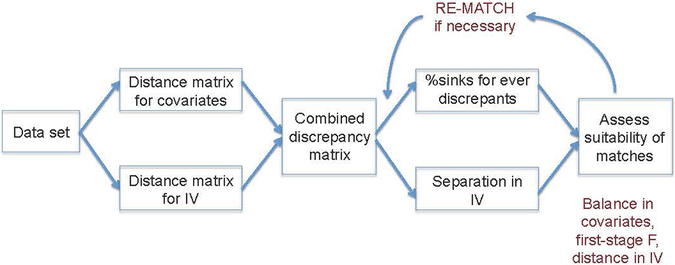
Conceptual illustration of near-far matching.
A near-far match applied to the education-wages example of Angrist and Krueger (1991) would match two individuals with similar age, race, marital status, and other measured confounders thought relevant to the education-wages relationship, who were born in different quarters of birth (ideally a quarter one with a quarter four birth). Near-far matches are controlled by two key parameters: The percent sinks is the percentage of data to be lost as unsuitable matches, and the cutpoint of differentiation for the IV specifies the difference in IV values in the pair match below which strong penalties are enforced. We find the percent sinks and cutpoint that maximize the F statistic measuring association between the IV and treatment, i.e., the percent sinks and cutpoint that strengthen the IV, and automate the near-far matching process to gain the benefits of the study design (reduced model dependency, nonparametric adjustment for measured confounders, and lowered mean squared error in for estimated causal effects).
Near-far matching is a study design technique. Study design refers to everything that happens before data analysis, including randomization scheme, inclusion/exclusion criteria, and ultimately data collection. Near-far matching can be thought of as “preprocessing” (Ho et al. 2007) of observational data to mimic a pair-randomized trial, as described above. It produces an analysis cohort that can then be used for inference on a target parameter. Inference refers to a post-study design process in which a scientifically meaningful target parameter is defined and statistical methods are used to make numerical statements about this parameter, e.g., effect size estimation and confidence intervals. A common inferential target in this setting is the complier average causal effect, as discussed in Angrist, Imbens, and Rubin (1996, Section 3.3) and Baiocchi et al. (2014, Section 4.1), equivalent to the effect ratio in Baiocchi et al. (2010, Section 3.2). Techniques for inference on the complier average causal effect include randomization inference (Baiocchi et al. 2010, Section 3.3), two-stage least squares regression (2SLS), and residual-inclusion models.
The purpose of this paper is to translate the prior foundational work on near-far matching (Baiocchi et al. 2010, 2012) into a package for R (R Core Team 2017), the nearfar package (Rigdon, Baiocchi, and Basu 2018) which is available from the Comprehensive R Archive Network (CRAN) at https://CRAN.R-project.org/package=nearfar, and to display the capabilities of nearfar through examples highlighting the advantages and caveats of near-far matching. In Section 2, we present an illustrative application of near-far matching to the education-wages inference problem introduced earlier. In Section 3, we present a simulated example in which the true causal treatment effect is known, and illustrate how near-far matching considerably may be able to strengthen a weak IV and reduce bias in an effect size estimate. In Section 4, we detail key analytical choices central to performing a near-far match. In Section 5, we present scenarios involving binary rather than continuous outcome variables, prioritized variables, and strengthening an IV without including measured covariates. We conclude with a discussion of limitations and next steps for research in Section 6.
2. An illustrative example
Consider the education-wages example discussed above, based on Angrist and Krueger (1991), where we hope to understand the effect of gaining more education on log of weekly earnings (wage). Suppose we consider a dataset with sample size n = 1000 from US census data for men born between 1930 and 1949. The sample size of 1000 is chosen to help the reader understand the percent sinks parameter in a near-far match, e.g., if percent sinks is 25%, then the resulting post-match sample size is n = 750. The data QOB.rar can be accessed from the web page http://economics.mit.edu/faculty/angrist/data1/data/angkru1991.
After downloading the data, we prepare a data frame df with n = 1000 randomly selected observations of log of weekly earned dollars of wages (wage), years of completed education (educ), measured covariates age (age in years), marital status (married; 1 if married, 0 otherwise), and race (race; 1 if black, 0 otherwise), quarter of birth (qob), and IV equal to 5−qob, such that 1 = 4th quarter of birth, 2 = 3rd quarter, 3 = 2nd quarter, and 4 = 1st quarter. The instrument IV is recoded so that smaller values encourage treatment, a coding convention required by the nearfar package. This dataset is included in our R package as angrist.
R> set.seed(1212)
R> library(“nearfar”)
R> head(angrist)
wage educ qob IV age married race
1 5.116621 12 1 4 43 1 0
2 5.367977 18 2 3 34 0 0
3 5.790019 12 1 4 35 1 0
4 6.380285 16 4 1 44 1 0
5 6.288895 10 1 4 46 1 0
6 5.790019 13 3 2 32 0 1
We are interested in the effect of education on earned wages. For individual j = 1,…, 1000, let Yj be the continuous outcome of interest, wage, Zj the treatment of interest, educ, and the vector of measured confounders, in this example, age, married, and race. The variable educ is continuous by nature, but is discretized in one-year intervals by Angrist and Krueger (1991). We choose to present educ as a continuous variable mainly for the purpose of exposition, as in practice researchers most commonly encounter binary, e.g., drug vs. placebo, or continuous, e.g., dose of drug or amount of radiation exposure, treatment variables. Finally, let be the vector of unmeasured confounders, e.g., access to opportunities or intellectual ability.
Figure 2 shows the bivariate relationship between education and log of weekly wages. Wages tend to increase with increasing education. A simple ordinary least squares (OLS) regression of education on wage yields a treatment effect of 0.076 (0.062, 0.090), where here and throughout the paper confidence intervals are found using the confint function from the stats package, a dependency of the nearfar package. The potential IV is uncorrelated with the error terms of this model (correlation = 0.00; 95% CI = (−0.07, 0.06)), indicating exogeneity. Using the same model and adjusting for the measured confounders of age, marital status, and race, the treatment effect estimate and error around the estimate is similar, at 0.077 (0.063, 0.090). The potential IV qob is again uncorrelated with the error terms of this model (correlation = 0.01; 95% CI = (−0.05, 0.07)), indicating exogeneity. Table 1 summarizes the variables of interest by qob.
Figure 2:
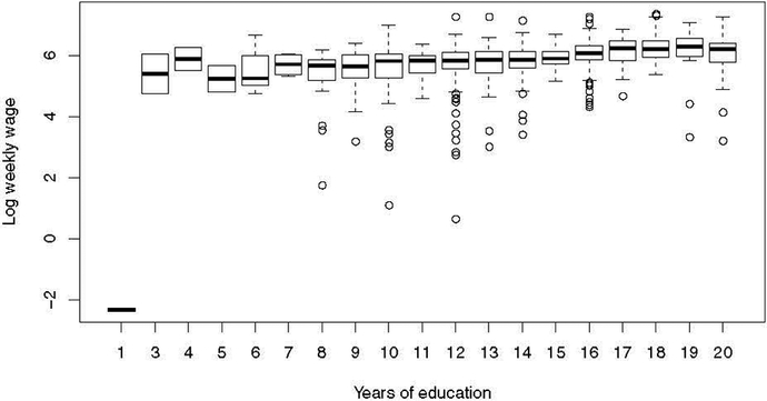
Education and log weekly wage in example.
Table 1:
Variables in example summarized by quarter of birth.
| Quarter of birth | |||||
|---|---|---|---|---|---|
| 1 | 2 | 3 | 4 | Total | |
| n = 215 | n = 270 | n = 271 | n = 244 | n = 1000 | |
| Log weekly wage | 5.8 (±0.7) | 5.8 (±0.8) | 5.8 (±0.6) | 5.8 (±0.7) | 5.8 (±0.7) |
| Years of education | 13.3 (±3.2) | 13.1 (±2.9) | 13.2 (±2.9) | 13.7 (±2.8) | 13.3 (±3.0) |
| Age (y) | 40.1 (±6.2) | 38.6 (±5.7) | 38.0 (±5.7) | 38.2 (±5.9) | 38.7 (±5.9) |
| Marriage status | |||||
| Unmarried | 37 (17.2%) | 42 (15.6%) | 47 (17.3%) | 45 (18.4%) | 171 (17.1%) |
| Married | 178 (82.8%) | 228 (84.4%) | 224 (82.7%) | 199 (81.6%) | 829 (82.9%) |
| Black race | |||||
| Not black | 197 (91.6%) | 243 (90.0%) | 242 (89.3%) | 227 (93.0%) | 909 (90.9%) |
| Black | 18 (8.4%) | 27 (10.0%) | 29 (10.7%) | 17 (7.0%) | 91 (9.1%) |
As expected, age decreases as qob increases. qob could be a valid IV as it increases education and is exogenous. In a simple regression of IV (as a factor variable) on education, the F statistic is 1.97 (df = 3 and 996, p = 0.12), meaning the IV is weak (< 10) (Stock and Yogo 2005).
R> df <- angrist
R> df$IV <- factor(df$IV)
R> l <- lm(educ ~ IV, data = df)
R> anova(l)
Analysis of Variance Table
Response: educ
Df Sum Sq Mean Sq F value Pr(>F)
IV 3 51.6 17.2135 1.9716 0.1166
Residuals 996 8695.9 8.7308
When adding age, marital status, and race to this regression, the partial F statistic is 1.93 (df = 3 and 993, p = 0.12), which is still weak (Stock and Yogo 2005).
Suppose we fit a two-stage least squares (2SLS) regression to estimate the effect of education on wages, despite the risk that such an estimate is biased and imprecise due to the weak IV (Bound et al. 1995; Small and Rosenbaum 2008). In the first stage, education is regressed on qob, age, marital status, and race, and in the second stage, wage is regressed on corrected age from the first stage, age, marital status, and race. Using the IV analysis, the treatment effect for education on wages is only 0.0080 (−0.18, 0.20) using the the ivreg function in the R package AER (Kleiber and Zeileis 2008).
R> m1i <- ivreg(wage ~ age + married + race + educ | IV + age + married +
+ race, data = df)
R> round(coefficients(summary(m1i)), digits = 4)
Estimate Std. Error t value Pr(>|t|)
(Intercept) 5.2740 1.6090 3.2778 0.0011
age 0.0078 0.0088 0.8865 0.3756
married1 0.2109 0.0607 3.4761 0.0005
race1 −0.3965 0.1238 −3.2017 0.0014
educ 0.0080 0.0976 0.0824 0.9343
We can illustrate how this estimate and its precision can change with near-far matching. After a distance matrix has been formed to reflect both the “near”-ness of individuals on the measured covariates and the simultaneous “far”-ness on the IV (details to follow in Section 4), the function opt_nearfar in the nearfar package uses a simulated annealing algorithm (from the GenSA package; Xiang, Gubian, Suomela, and Hoeng 2013) to find the percent sinks and cutpoint maximizing the partial F statistic from a regression of the treatment on the IV (and including, optionally, measured confounders) through calling the nonbipartite matching algorithm implemented in the nbpMatching package (Lu, Greevy, Xu, and Beck 2011). We caution that the opt_nearfar function relies on stochastic rather than deterministic optimization and thus offers no optimality guarantees, and is an algorithmic approach designed to offer guidance on how to choose the parameters of the near-far match, the percent sinks and the separation in the IV. The user must still check balance post-match and may want to contrast results from other near-far matches.
To apply the opt_nearfar function to our problem, we must specify the following minimal set of arguments in opt_nearfar: dta is the name of the data frame, trt is the name of the treatment variable, iv is the name of the IV, and covs is a vector of the names of the covariates we wish to adjust for, e.g., covs = c(“age”, “sex”, “race”). If the treatment variable is binary, set trt.type = “bin” (default is continuous, i.e., trt.type = “cont”). The IV should be coded such that smaller values encourage individuals into a higher dosage of the treatment. In our example, the variable IV is recoded as 5‒qob so that an individual born in the 4th quarter is encouraged into the most education.
Additional optional parameters in opt_nearfar include a list of named measured covariates to prioritize in the match, where the default is that all covariates are of equal priority (imp.var; default = NA), their corresponding levels of importance, where the default is equal importance (tol.var; default = NA), the range of percent sinks over which to maximize the F statistic (sink.range; default = [0, 0.5]) such that maximally 50% of data can be removed, the range of IV cutpoint values over which to maximize the F statistic (cutpoint.range; default = [one SD of IV, length of range of IV]), an indicator of whether or not to adjust for measured covariates when optimizing the first stage F statistic (adjust.IV; default = TRUE), and the amount of time to let the algorithm run (max.time.seconds; default = 300, or 5 minutes). In Section 4, more details will be presented regarding altering these specifications, but for now we focus on a simple near-far match with a 10 minute run time to increase reproducibility of the results (with a shorter run time of 5 minutes, the simulated annealing algorithm is more likely to yield differing study designs across repeated executions of the code):
R> k <- opt_nearfar(dta = df, trt = “educ”, covs = c(“age”, “married”,
+ “race”), iv = “IV”, trt.type = “cont”, imp.var = NA, tol.var = NA,
+ adjust.IV = TRUE, max.time.seconds = 600)
R> summary(k)
Starting sample size: 1000
Starting F-value: 1.93
Maximum F-value: 3.01
Number of study designs tried: 735
Cutpoint in IV at max F: 2.75
Percent sink at max F: 47.69
Sample size at max F: 522 (261 pair matches)
Summary of balance at optimal match:
Encouraged n=261 Discouraged n=261 Abs St Dif
IV 1.39463602 3.50574713 4.261847
age 38.34482759 38.34482759 0.000000
married 0.85057471 0.85057471 0.000000
race 0.04980843 0.04980843 0.000000
In the above, note that the near-far match object, k, contains eight elements: the number of calls to the objective function (n.calls; or the number of matches performed in the search algorithm for the optimal match), the range over which to search for optimal percent sinks (sink.range), the range over which to search for an optimal IV cutpoint (cutp.range), the optimal percent sink found (pct.sink), the optimal cutpoint found (cutp), the maximum F statistic (maxF), the two-column matrix of matches wherein the first column is the list of indices of encouraged individuals (those for whom the IV would favor entry into treatment if treatment is binary, or more treatment if treatment is continuous) and the second column is the corresponding list of discouraged individuals (those for whom the IV would favor entry into placebo if treatment is binary, or less treatment if treatment is continuous; match), and finally a three-column summary of the match wherein the first column is the post-match mean among encouraged individuals, the second column is the post-match mean among discouraged individuals, and the third column is the absolute standardized difference between the encouraged and discouraged individuals (summ). The summary feature exists to summarize key elements of the near-far match, and its results are displayed above.
Table 2 summarizes the balance statistics in the example n = 1000 dataset, both pre- and post-near-far match with a 10 minute run time. After letting the simulated annealing algorithm run for 10 minutes, the partial F statistic increased to 3.01 (indicating that in this example, quarter of birth remains a weak IV for education), the optimal cutpoint equal to 2.75, and the optimal percent sinks to 48%, reducing the dataset to n = 522 post-near-far match. This example thus illustrates key limitations for the analyst to be aware of when performing a near-far match, particularly with default application package settings: That the F statistic is not guaranteed to be stronger than common rules-of-thumb (> 10 or > 13) for IV strength after near-far matching, that data will be lost in a match such that the treatment effect will remain a local treatment effect as with all IV analyses (not an effect estimate generalizable to all persons), and thus there will be a balance between strengthening inference in terms of reducing bias and mean squared error and reducing generalizability in the analysis by throwing out individuals from the analytical sample. We discuss these issues further in the discussion in Section 6.
Table 2:
Variable summaries in example pre- and post-near-far match (ASD = absolute standardized difference).
| Pre-match | Post-match | |||||
|---|---|---|---|---|---|---|
| Encouraged n = 515 |
Discouraged n = 485 |
ASD | Encouraged n = 261 |
Discouraged n = 261 |
ASD | |
| IV | 1.53 | 3.44 | 3.85 | 1.39 | 3.51 | 4.26 |
| Age (y) | 38.08 | 39.28 | 0.20 | 38.34 | 38.34 | 0.00 |
| Married (%) | 0.82 | 0.84 | 0.04 | 0.85 | 0.85 | 0.00 |
| Race (% black) | 0.09 | 0.09 | 0.01 | 0.05 | 0.05 | 0.00 |
Table 3 compares the inferential results from above to those post-near-far match. Notably, after the match, the conclusion is reached that education increases log weekly wage whereas pre-near-far match no effect was seen. We also conducted inference on the effect ratio post-near-far match as in Baiocchi et al. (2010, Section 3.3). Inference on the effect ratio is available using the function eff_ratio. Furthermore, the mean squared error around the 2SLS estimate is smaller than in the OLS case where unobserved confounders were not accounted for; as shown in Table 3, the estimated effect of education on earnings has a lower standard error (0.076 post-match versus 0.098 pre-match). Figures 2 and 4 of Ho et al. (2007) show reduced model dependency after matching. In Figure 3, we computed the treatment effect for all second stage 2SLS main effects models including education and including age, marital status, and race, for a total of models, both pre-near-far match and post-near-far match.
Table 3:
Estimates (confidence intervals) for treatment effect of one-year increase in education on log weekly wages.
| OLS unadjusted | OLS adjusted | 2SLS | Effect ratio | |
|---|---|---|---|---|
| Pre-near-far | 0.076 | 0.077 | 0.0080 | |
| (0.062, 0.090) | (0.063, 0.090) | (−0.18, 0.20) | ||
| Post-near-far | 0.064 | 0.064 | 0.10 | 0.13 |
| (0.044, 0.083) | (0.045, 0.083) | (−0.048, 0.25) | (–, –) |
Figure 3:
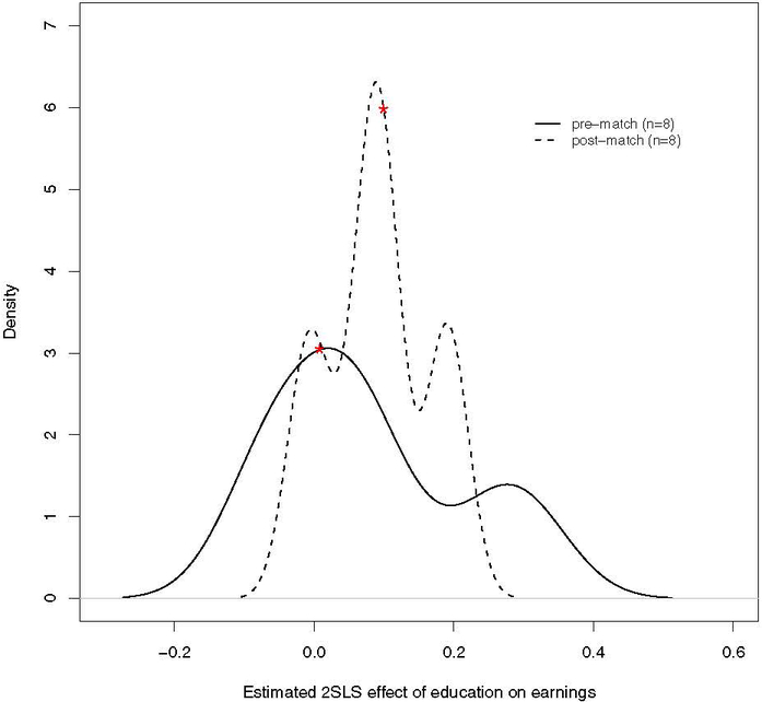
Kernel density plots of treatment effect estimates of education on earnings pre- and post-near-far match. Red stars denote treatment effects summarized in Table 2.
It is evident from Figure 3 that the near-far match reduces model dependency as all estimates are more tightly clustered. Nevertheless, because the F statistic remained < 10, we would suggest a stronger IV would still be necessary to perform unbiased effect estimation. In the next section, we illustrate an example where such a strong IV is achieved using opt_nearfar.
3. Simulated example
In the education and wage example presented in Section 2, we were able to strengthen the qob IV (strength measured by partial F statistic) from 1.93 to only 3.01 using the near-far match. In this section, we present a simulated example where we are able to increase the partial F statistic from < 10 (weak) to > 13 (strong enough to meet commonly-used criteria for inference; Stock and Yogo 2005).
For illustration, we mimic a simulation setup previously presented by Simmering (2014). To generate the data (including unmeasured confounders), we first simultaneously generate the latent part of treatment (Zstar) that is correlated with measured (X.meas) and unmeasured confounders (X.meas) using MASS (Venables and Ripley 2002). Then we generate an IV (IV), an observed treatment (Z), and an observed outcome (Y), and set the data up for a near-far match (df.sim) as follows:
R> set.seed(172)
R> library(“MASS”)
R> dta <- mvrnorm(1000, c(10, 10, 10),
+ matrix(c(1, −0.5, 0.5, −0.5, 1, 0.5, 0.5, 0.5, 1), 3, 3))
R> Zstar <- dta[, 1]
R> X.unmeas <- dta[, 2]
R> X.meas <- dta[, 3]
R> IV <- rnorm(1000, 10, 1)
R> Z <- 1 + 5 * Zstar + 3 * X.meas + 1 * IV + rnorm(1000, 0, 10)
R> Y <- 1 + 1 * Z + 1 * X.meas + 5 * X.unmeas + rnorm(1000, 0, 20)
R> df.sim <- data.frame(Y = Y, Z = Z, IV = IV, X = X.meas)
R> head(df.sim)
Y Z IV X
1 166.6706 90.66159 11.69692 9.196521
2 194.1678 106.80978 10.93272 11.216561
3 205.1344 94.94531 10.81390 11.436570
4 122.2822 75.52858 10.33122 8.566827
5 154.3247 88.80118 8.34264 10.325343
6 125.7180 86.83526 10.44303 10.071408
The true treatment effect of the treatment Z on the outcome Y is equal to 1. IV is an instrumental variable for Z because it is related to Z while remaining unrelated to the outcome Y (except through Z) and unmeasured confounder X.unmeas. X.unmeas is not available for analysis, and thus a regression model for Y without X.unmeas will not recover the true treatment effect. In the true model, lm(Y ~ Z + X.unmeas + X.meas), the estimated treatment effect is 0.98 (0.85, 1.10) in our simulated dataset where noise was added as shown above, and in the model without the unmeasured confounder, lm(Y ~ Z + X, data = df.sim), the estimated treatment effect is 0.81 (0.70, 0.93). IV is a weak instrument for Z as the partial F statistic is only 7.87. The 2SLS model, ivreg(Y ~ X + Z | IV + X, data = df.sim), estimates the treatment effect as 0.49 (−0.83, 1.81), revealing both bias and large error around the estimate.
Applying the near-far matching package to the data in df.sim strengthens the F statistic and improves estimation of the treatment effect of Z on Y using the filtered cohort:
R> nf <- opt_nearfar(dta = df.sim, trt = “Z”, covs = “X”, iv = “IV”,
+ trt.type = “cont”, imp.var = NA, tol.var = NA, adjust.IV = TRUE,
+ max.time.seconds = 600)
R> summary(nf)
Starting sample size: 1000
Starting F-value: 7.87
Maximum F-value: 10.79
Number of study designs tried: 232
Cutpoint in IV at max F: 1.03
Percent sink at max F: 29.94
Sample size at max F: 700 (350 pair matches)
Summary of balance at optimal match:
Encouraged n=350 Discouraged n=350 Abs St Dif
IV 9.209574 10.847513 2.531430015
X 9.981922 9.979881 0.002060996
The near-far match filters the cohort from n = 1000 to n = 700 (350 pair matches) and increases the partial F statistic to 10.79. The treatment effect in the filtered cohort is estimated as 0.99 (0.85, 1.14) in the true model, 0.82 (0.68, 0.96) in OLS without the unmeasured confounder, 0.76 (−0.34, 1.86) in 2SLS, and finally 0.93 (−0.79, 2.98) by the nonparametric effect ratio procedure. In the 2SLS model, the near-far match yields narrower confidence intervals (standard error post-match down to 0.56 from 0.67 pre-match) in addition to less bias in estimating the treatment effect (0.76 post-match versus 0.49 pre-match), revealing both higher precision and higher accuracy in the effect size estimation.
4. Key analytical choices
In this section we look at the key analytical choices in the package design to implement near-far matching.
The first step in the package implementation of the near-far matching method is the construction of an n × n measured confounder distance matrix for the n individuals in the study. The distance matrix is constructed using only pre-treatment covariates. In contrast, the distance matrix for propensity score matching is of smaller dimension but explicitly uses the treatment assignments, i.e., the rows of the distance matrix are the treated and the columns of the distance matrix are the controls. The larger distance matrix in the near-far setting is warranted because we do not assume strongly ignorable treatment assignment (SITA). SITA simplifies the problem because conditional on the covariates that are used to build the propensity score, treatment assignment is assumed to be independent of potential outcomes, allowing matching of treated to controls to lead to unbiased estimates of the average treatment effect (Rosen-baum 1984, Section 2.6). The near-far approach does not assume SITA. Instead, the potential outcomes of two units that have the same observed covariates may still not be independent of treatment assignment, and matching treated to controls on observed covariates through the propensity score will not be enough to yield unbiased estimation of the average treatment effect. We attempt to control for unmeasured confounders through use of an instrumental variable as detailed further in the paragraphs to follow.
We use rank-based Mahalanobis distance on observed covariates to compute the distance matrix and limit the impact of any extreme distributions (Rubin 1979; Greevy, Lu, Silber, and Rosenbaum 2004). This procedure is applied to the measured confounders age, married, and race in df2 as follows:
R> aa <- angrist[, 5:7]
R> head(aa)
age married race
1 43 1 0
2 34 0 0
3 35 1 0
4 44 1 0
5 46 1 0
6 32 0 1
R> X2 <- matrix(as.numeric(as.matrix(aa)), dim(aa)[1], dim(aa)[2])
R> jj <- smahal(X2)
R> round(jj[1:5, 1:5], 2)
[,1] [,2] [,3] [,4] [,5]
[1,] 0.00 4.82 1.64 0.02 0.18
[2,] 4.82 0.00 3.07 5.24 6.14
[3,] 1.64 3.07 0.00 2.05 2.91
[4,] 0.02 5.24 2.05 0.00 0.08
[5,] 0.18 6.14 2.91 0.08 0.00
Individuals have 0 distance to themselves on the diagonal of the distance matrix jj above. Additionally, pairs of individuals with similar measured confounders, e.g., individuals 1 and 4, have much smaller distances than pairs of individuals with different measured confounders, e.g., individuals 1 and 2. The rank-based Mahalanobis distance between 1 and 4 is only 0.02 whereas the distance between 1 and 2 is 4.82.
Suppose that it is vitally important to match individuals as closely as possible on one of the measured confounders, say age. The calipers function recomputes the distance matrix to prioritize age as follows:
R> jj2 <- calipers(jj, aa$age, tolerance = 0.2)
R> round(jj2[1:5, 1:5], 2)
[,1] [,2] [,3] [,4] [,5]
[1,] 0.00 7.06 3.63 0.02 0.93
[2,] 7.06 0.00 3.07 7.74 9.13
[3,] 3.63 3.07 0.00 4.29 5.66
[4,] 0.02 7.74 4.29 0.00 0.58
[5,] 0.93 9.13 5.66 0.58 0.00
Above we see that individuals 1 and 2 have moved farther apart (distance increases from 4.82 to 7.06) after prioritizing a close match on age. Individuals 1 and 4 remain close at a distance of 0.02. As in Baiocchi et al. (2010), for all of pairs in jj for which the absolute difference between the age variable is greater than tolerance times the standard deviation of age, a penalty of one half times the standard deviation of all distances in jj times the original pair distance divided by the standard deviation of age is added to the original distance in jj to yield jj2. As such, a value of tolerance = 0 would penalize pairs that are not exactly matched on age, and increasing values of tolerance away from 0 are less likely to penalize. For example, a tolerance value of 1 would only penalize those pairs for which the absolute difference in age is greater than one standard deviation of age. The default value of tolerance is set to 0.2 so that pairs with an absolute difference of 20% of a standard deviation or more on the corresponding imp.var are penalized. The opt_nearfar function allows for up to five variables in imp.var (along with five specified tolerances in tol.var) such that the distance matrix jj can be updated five times. The order of variables in imp.var does matter as the distance matrix jj is sequentially updated.
After any updates to the distance matrix have taken place using calipers, the next step in the near-far match is to penalize pairs in the distance matrix that have values of the IV that are too close. This is accomplished by the function matches within the package nearfar. For all of pairs in jj for which the absolute difference between the IV variable is less than the user specified argument cutpoint, a penalty of the maximum of all absolute differences among these pairs minus the standard deviation of the distance matrix of all pairs is added to yield an updated distance matrix. At this point in the near-far matching process, we have a distance matrix that whose distances reflect near-ness on measured confounders and far-ness on the IV. The matches function finishes by calling the nonbimatch function within nbpMatching to find the set of pairwise matches that minimizes the sum of distances between the pairs.
Note that prior to applying nonbimatch to find the optimal non-bipartite match, users should consider that many of the individuals may have uniformly large distances to all other individuals and thus are consistently discordant with the sample. These consistently discordant individuals are precisely the individuals whose removal will improve inference on the treatment effect in terms of bias and variance. The sinks argument within the matches function allows for the removal of n·sinks individuals as follows. First, n sinks rows and columns of 0s are added to the distance matrix such that the n·sinks have zero distance to all individuals in the distance matrix. The n·sinks diagonal elements of the added rows and columns are set to the maximum of the distance matrix times three to ensure that sinks do not match to sinks. After creating the distance matrix with sinks, the user can run nonbimatch and the n·sinks most consistently discordant individuals are matched to sinks while the remaining n · (1−sinks) individuals are pair matched to minimize the sum of distances between the pairs. The near-far match is now complete.
Thus, after fixing the the prioritized variables in imp.var and corresponding tolerances in tol.var, there are two free user-defined parameters that control the design of the near-far match: cutpoint and sink. The final part of the opt_nearfar function automates the discovery of the two free parameters that strengthen the near-far match, i.e., maximizing the F statistic (or deviance if trt.type = “bin”) for the IV in a regression of the IV on the treatment. If adjust.IV = TRUE, all measured covariates are included in this regression. As mentioned above in Section 2, the user can specify the potential range of sinks, sink.range (default = [0, 0.5]), and also the potential range of cutpoints (default = [one SD of IV, length of range of IV]) to search across. After specifying these ranges, opt_nearfar calls the GenSA function (Xiang et al. 2013) to find the optimal near-far cutpoint and sink study design parameters. We again caution the user that GenSA and thus opt_nearfar rely upon a stochastic optimization algorithm that is not guaranteed to yield the same results in repeated runs of the same code.
5. Special scenarios
In this section, we will cover specific scenarios that arise in practice: (1) a case in which the treatment of interest is binary; (2) an example where the analyst wishes to prioritize some variables in the near-far match, and (3) a case where the analyst does not wish to adjust for measured confounders when optimizing the first stage F statistic (i.e., still matching on confounders, but calculating the F statistic strength of the IV without including such confounders, as is common in some epidemiological literature to capture the weakest-possible F statistic for a given IV).
5.1. Binary treatment
Suppose an analyst is interested in the same problem discussed in Section 2, the effect of education (in years) on log of weekly wages, but we only had a binary (Burgess, Thompson, and CRP CHD Genetics Collaboration 2011) indicator of education greater than high school, as follows:
R> df3 <- data.frame(wage = angrist$wage,
+ educ = ifelse(angrist$educ > 12, 1, 0), IV = factor(angrist$IV),
+ age = angrist$age, married = factor(angrist$married),
+ race = factor(angrist$race))
R> head(df3)
wage educ IV age married race
1 5.116621 0 4 43 1 0
2 5.367977 1 3 34 0 0
3 5.790019 0 4 35 1 0
4 6.380285 1 1 44 1 0
5 6.288895 0 4 46 1 0
6 5.790019 1 2 32 0 1
We need to understand how strong the relationship is between the IV and the treatment of interest, binary education. The partial deviance statistic with a binary outcome is a reasonable analog to the partial F statistic with a continuous outcome. It is calculated as follows:
R> m3 <- glm(educ ~ age + married + race + IV, data = df3,
+ family = binomial)
R> anova(m3)
Analysis of Deviance Table
Model: binomial, link: logit
Response: educ
Terms added sequentially (first to last)
Df Deviance Resid. Df Resid. Dev
NULL 999 1385.6
age 1 21.4100 998 1364.2
married 1 0.2068 997 1364.0
race 1 14.6932 996 1349.3
IV 3 3.2916 993 1346.0
The IV must be added last when defining the model to calculate its partial deviance, e.g., IV is the last term in the formula educ ~ age + married + race + IV above. The IV is weak as the partial deviance is only 3.29. The opt_nearfar function can be used to perform near-far matching as follows:
R> set.seed(44)
R> nf2 <- opt_nearfar(dta = df3, trt = “educ”, covs = c(“age”, “married”,
+ “race”), iv = “IV”, trt.type = “bin”, imp.var = NA, tol.var = NA,
+ adjust.IV = TRUE, max.time.seconds = 600)
R> summary(nf2)
Starting sample size: 1000
Starting F-value: 3.29
Maximum F-value: 13.09
Number of study designs tried: 626
Cutpoint in IV at max F: 2.29
Percent sink at max F: 47.69
Sample size at max F: 522 (261 pair matches)
Summary of balance at optimal match:
Encouraged n=261 Discouraged n=261 Abs St Dif
IV 1.39463602 3.50574713 4.261847
age 38.34482759 38.34482759 0.000000
married 0.85057471 0.85057471 0.000000
race 0.04980843 0.04980843 0.000000
In this case, the partial deviance has increased to 13.09, with 48% sinks and a cutpoint of 2.29 to yield n = 261 pair matches. Note the similarity in these results to the results above where education was continuous (48% sinks and cutpoint 2.75, such that there were also n = 261 pair matches).
Applying a one to one Mahalanobis based match within a caliper of 2 pooled standard deviations of the propensity score (estimated by a logistic regression of educ as a function of age, married, and race), an interested user can compare and contrast near-far matching with propensity score matching (PSM implemented in optmatch; Hansen and Klopfer 2006).
R> library(“optmatch”)
R> ppty <- glm(educ ~ age + married + race, family = binomial, data = df3) R> mhd <- match_on(educ ~ age + married + race, data = df3) +
+ caliper(match_on(ppty), 2)
R> pm <- pairmatch(mhd, data = df3)
R> summary(pm)
Structure of matched sets:
1:1 0:1
487 26
Effective Sample Size: 487
(equivalent number of matched pairs).
The post-match results from near-far and PSM can be compared in a simple linear model of wage on binary educ while adjusting for age, married, and race. The coefficient for educ in this model is estimated as 0.27 (0.16, 0.38) in the n = 522 post-near-far dataset and 0.31 (0.23, 0.40) in the n = 974 post-PSM dataset. For reference, the effect estimate in the n = 1000 pre-match data is 0.31 (0.23, 0.40).
5.2. Prioritized variables in near-far match
Suppose now that there is a subset of measured confounders, e.g., age and married, that the analyst wishes to prioritize in the match. In other words, age and married should be given priority to be as near as possible in the near-far match. The argument imp.var will take the names of the variables to be prioritized and the argument tol.var will take the corresponding tolerance values. A tolerance value of 0 only allows for exact matches in all of the pairs, and an increasing tolerance allows for more discrepancy between individual pair matches with regard to the corresponding variable. To prioritize age and married in the match, the package would be used as follows:
R> set.seed(33)
R> nf3 <- opt_nearfar(dta = df3, trt = “educ”, covs = c(“age”, “married”,
+ “race”), iv = “IV”, trt.type = “bin”, imp.var = c(“age”, “married”),
+ tol.var = c(0.3,0.2), adjust.IV = TRUE, max.time.seconds = 600)
R> summary(nf3)
Starting sample size: 1000
Starting F-value: 3.29
Maximum F-value: 13.09
Number of study designs tried: 636
Cutpoint in IV at max F: 2.43
Percent sink at max F: 47.62
Sample size at max F: 522 (261 pair matches)
Summary of balance at optimal match:
Encouraged n=261 Discouraged n=261 Abs St Dif
IV 1.39463602 3.50574713 4.261847
age 38.34482759 38.34482759 0.000000
married 0.85057471 0.85057471 0.000000
race 0.04980843 0.04980843 0.000000
5.3. No adjustment for measured confounders
Now suppose the analyst wanted to maximize the F statistic from an unadjusted model of the treatment regressed on the IV without unmeasured confounders. The function opt_nearfar includes the adjust.IV argument specifically for this purpose. In the following example, we again have a binary treatment (educ; education greater than 12 years), the IV quarter of birth, and the measured confounders age, married, and race. Note that even with adjust.IV = FALSE, individuals are still matched to be near on the measured confounders listed above and far on the IV, but the target to be maximized has changed from the partial deviance for IV from glm(educ ~ age + married + race + IV, family = binomial) to the deviance for IV from glm(educ ~ IV, family = binomial). The following code implements this study design:
R> set.seed(53)
R> nf4 <- opt_nearfar(dta = df3, trt = “educ”, covs = c(“age”, “married”,
+ “race”), iv = “IV”, trt.type = “bin”, imp.var = NA, tol.var = NA,
+ adjust.IV = FALSE, max.time.seconds = 600)
R> summary(nf4)
Starting sample size: 1000
Starting F-value: 3.63
Maximum F-value: 12.91
Number of study designs tried: 718
Cutpoint in IV at max F: 2.86
Percent sink at max F: 47.66
Sample size at max F: 522 (261 pair matches)
Summary of balance at optimal match:
Encouraged n=261 Discouraged n=261 Abs St Dif
IV 1.39463602 3.50574713 4.261847
age 38.34482759 38.34482759 0.000000
married 0.85057471 0.85057471 0.000000
race 0.04980843 0.04980843 0.000000
Note the similarity of all of the results in Sections 5.1, 5.2 and 5.3. All three of the study designs called the objective function over 600 times, yielding partial deviance statistics above 12.9, and resulted in pair-matches of n = 261 pairs, n = 261 pairs, and n = 261 pairs, respectively.
6. Discussion
“Give me six hours to chop down a tree and I will spend the first four sharpening the axe.”
– Abraham Lincoln
Here, we detailed a newly-available R software package nearfar (Rigdon et al. 2018) that enables analysts to implement the study design (pre-inference) method of “near-far matching”, which “filters” data from a cohort by simultaneously matching individuals within the cohort to be “near” (similar) on measured confounders and “far” (different) on levels of an IV. We illustrated, using both a classical example and a simulated dataset, how the package can be used to “strengthen” a weak IV by adjusting the “near-ness” and “far-ness” of a match, reduce model dependency, enable nonparametric adjustment for measured confounders, and lower mean squared error in estimated causal effects of a treatment or intervention. We additionally illustrated how to utilize the nearfar package when analyzing either continuous or binary outcomes, how to prioritize variables in the match, and how to calculate F statistics of IV strength with or without adjustment for measured covariates.
As with any analytic method, the near-far approach and the package to implement it have important limitations. As illustrated in Section 2, the F statistic is not guaranteed to be stronger than common rules-of-thumb (> 10 or > 13) for IV strength after near-far matching. Our optimizer function, opt_nearfar, does not offer any optimality guarantees, and is added to the package to offer the user guidance on where to look in the two-dimensional study design space, defined by percent sinks and separation in the IV, for near-far matches that will strengthen the instrument. We encourage the user to try additional near-far matches to those suggested by opt_nearfar as sensitivity analyses. Further simulation based research is needed to compare and contrast near-far matching to propensity score matching when addressing the impact of unmeasured confounding. Additionally, as nearfar only currently works for binary and continuous treatment variables, strengthening an instrument using near-far matching in the context of an ordinal treatment variable merits further research. Finally, as with any matching-based method, data will be lost in a match such that the treatment effect will remain a local treatment effect as with all IV analyses (not an effect estimate generalizable to all persons), and thus there will be a balance between strengthening inference in terms of reducing bias and mean squared error and reducing generalizability in the analysis by throwing out individuals from the analytical sample.
Near-far matching is, nevertheless, a useful study design approach to address several classical problems with observational inference: the desire to include an IV to address unmeasured confounders, the difficulty of finding a strongly randomizing IV, and the need to adjust for measured confounders. Near-far matching is not the only method to strengthen an IV; new weighting methods are under development (Lehmann, Li, Saran, and Li 2016). More advanced users of matching may be able to implement near-far matching in the R package designmatch (Zubizarreta, Kilcioglu, and Vielma 2018), though this package has dependencies only available to academic researchers and does not include tools for finding an optimal near-far match. Any of the familiar tools for IVs, e.g., two-stage least squares, can be applied post near-far match, with the benefit that the package presented here may help the analyst reduce model dependency, nonparametrically adjust for measured confounders, and reduce mean squared error in the estimation of the treatment effect. Hence, nearfar provides a potentially useful tool to create a high-quality cohort from large observational data.
Acknowledgments
Research reported in this publication was supported by the National Institute On Minority Health And Health Disparities of the National Institutes of Health under Award Number DP2MD010478. Additional support was provided by the Agency for Healthcare Research and Quality of the National Institutes of Health under Award Number 5R00HS022192–03. The content is solely the responsibility of the authors and does not necessarily represent the official views of the National Institutes of Health.
Contributor Information
Joseph Rigdon, Stanford University.
Michael Baiocchi, Stanford University.
Sanjay Basu, Stanford University.
References
- Angrist JD, Imbens GW, Rubin DB (1996). “Identification of Causal Effects Using Instrumental Variables.” Journal of the American Statistical Association, 91(434), 444–455. doi: 10.1080/01621459.1996.10476902. [DOI] [Google Scholar]
- Angrist JD, Krueger AB (1991). “Does Compulsory School Attendance Affect Schooling and Earnings?” The Quarterly Journal of Economics, 106(4), 979–1014. doi: 10.2307/2937954. [DOI] [Google Scholar]
- Baiocchi M, Cheng J, Small DS (2014). “Instrumental Variable Methods for Causal Inference.” Statistics in Medicine, 33(13), 2297–2340. doi: 10.1002/sim.6128. [DOI] [PMC free article] [PubMed] [Google Scholar]
- Baiocchi M, Small DS, Lorch S, Rosenbaum PR (2010). “Building a Stronger Instrument in an Observational Study of Perinatal Care for Premature Infants.” Journal of the American Statistical Association, 105(492), 1285–1296. doi: 10.1198/jasa.2010.ap09490. [DOI] [Google Scholar]
- Baiocchi M, Small DS, Yang L, Polsky D, Groeneveld PW (2012). “Near/Far Matching: A Study Design Approach to Instrumental Variables.” Health Services and Outcomes Research Methodology, 12(4), 237–253. doi: 10.1007/s10742-012-0091-0. [DOI] [PMC free article] [PubMed] [Google Scholar]
- Bound J, Jaeger DA, Baker RM (1995). “Problems with Instrumental Variables Estimation When the Correlation between the Instruments and the Endogenous Explanatory Variable Is Weak.” Journal of the American Statistical Association, 90(430), 443–450. doi: 10.1080/01621459.1995.10476536. [DOI] [Google Scholar]
- Burgess S, Thompson SG, CRP CHD Genetics Collaboration (2011). “Avoiding Bias from Weak Instruments in Mendelian Randomization Studies.” International Journal of Epidemiology, 40(3), 755–764. doi: 10.1093/ije/dyr036. [DOI] [PubMed] [Google Scholar]
- Cawley J, Conneely K, Heckman J, Vytlacil E (1997). “Cognitive Ability, Wages, and Meritocracy” In Intelligence, Genes, and Success, pp. 179–192. Springer-Verlag. [Google Scholar]
- Greevy R, Lu B, Silber JH, Rosenbaum P (2004). “Optimal Multivariate Matching before Randomization.” Biostatistics, 5(2), 263–275. doi: 10.1093/biostatistics/5.2.263. [DOI] [PubMed] [Google Scholar]
- Hammond EC (1964). “Smoking in Relation to Mortality And Morbidity. Findings in First Thirty-Four Months of Follow-Up in a Prospective Study Started in 1959.” Journal of the National Cancer Institute, 32(5), 1161–1188. doi: 10.1093/jnci/32.5.1161. [DOI] [PubMed] [Google Scholar]
- Hansen BB, Klopfer SO (2006). “Optimal Full Matching and Related Designs via Network Flows.” Journal of Computational and Graphical Statistics, 15(3), 609–627. doi: 10.1198/106186006x137047. [DOI] [Google Scholar]
- Ho DE, Imai K, King G, Stuart EA (2007). “Matching as Nonparametric Preprocessing for Reducing Model Dependence in Parametric Causal Inference.” Political Analysis, 15(3), 199–236. doi: 10.1093/pan/mpl013. [DOI] [Google Scholar]
- Kleiber C, Zeileis A (2008). Applied Econometrics with R. Springer-Verlag, New York. doi:10.1007/978-0-387-77318-6 . URL 10.1007/978-0-387-77318-6https://CRAN.R-project.org/package=AER. URL https://CRAN.R-project.org/package=AER . [DOI] [Google Scholar]
- Lehmann D, Li Y, Saran R, Li Y (2016). “Strengthening Instrumental Variables through Weighting.” Statistics in Biosciences, 9(2), 320–338. doi: 10.1007/s12561-016-9149-9. [DOI] [PMC free article] [PubMed] [Google Scholar]
- Lu B, Greevy R, Xu X, Beck C (2011). “Optimal Nonbipartite Matching and Its Statistical Applications.” The American Statistician, 65(1), 21–30. doi: 10.1198/tast.2011.08294. [DOI] [PMC free article] [PubMed] [Google Scholar]
- Mayer SE, Jencks C (1989). “Growing Up in Poor Neighborhoods: How Much Does It Matter.” Science, 243(4897), 1441–1445. doi: 10.1126/science.243.4897.1441. [DOI] [PubMed] [Google Scholar]
- R Core Team (2017). R: A Language and Environment for Statistical Computing R Foundation for Statistical Computing, Vienna, Austria: URL https://www.R-project.org/. [Google Scholar]
- Rigdon J, Baiocchi M, Basu S (2018). nearfar: Near-Far Matching. R package version 1.2, URL https://CRAN.R-project.org/package=nearfar. [DOI] [PMC free article] [PubMed] [Google Scholar]
- Rosenbaum PR (1984). “From Association to Causation in Observational Studies: The Role of Tests of Strongly Ignorable Treatment Assignment.” Journal of the American Statistical Association, 79(385), 41–48. doi: 10.2307/2288332. [DOI] [Google Scholar]
- Rosenbaum PR (2002). Observational Studies. Springer-Verlag, New York. [Google Scholar]
- Rubin DB (1979). “Using Multivariate Matched Sampling and Regression Adjustment to Control Bias in Observational Studies.” Journal of the American Statistical Association, 74(366a), 318–328. doi: 10.1080/01621459.1979.10482513. [DOI] [Google Scholar]
- Simmering J (2014). “Instrumental Variables Simulation.” http://jacobsimmering.com/page2/. Accessed: 2016-07-18. [Google Scholar]
- Small DS, Rosenbaum PR (2008). “War and Wages: The Strength of Instrumental Variables and Their Sensitivity to Unobserved Biases.” Journal of the American Statistical Association, 103(483), 924–933. doi: 10.1198/016214507000001247. [DOI] [Google Scholar]
- Stock JH, Yogo M (2005). “Testing for Weak Instruments in Linear IV Regression” In DWK Andrews, Stock JH (eds.), Identification and Inference for Econometric Models: Essays in Honor of Thomas Rothenberg, pp. 80–108. Cambridge University Press, Cambridge. doi: 10.1017/cbo9780511614491.006. [DOI] [Google Scholar]
- Venables WN, Ripley BD (2002). Modern Applied Statistics with S. 4th edition Springer-Verlag, New York. [Google Scholar]
- Xiang Y, Gubian S, Suomela B, Hoeng J (2013). “Generalized Simulated Annealing for Efficient Global Optimization: The GenSA Package for R.” The R Journal, 5(1), 13–28. [Google Scholar]
- Zubizarreta JR, Kilcioglu C, Vielma JP (2018). designmatch: Matched Samples That Are Balanced and Representative by Design. R package version 0.3.1, URL https://CRAN.R-project.org/package=designmatch. [Google Scholar]