Abstract
Portable wireless ultrasound has been emerging as a new ultrasound device due to its unique advantages including small size, lightweight, wireless connectivity and affordability. Modern portable ultrasound devices can offer high quality sonogram images and even multiple ultrasound modes such as color Doppler, echocardiography, and endovaginal examination. However, none of them can provide elastography function yet due to the limitations in computational performance and data transfer speed of wireless communication. Also phase-based strain estimator (PSE) that is commonly used for conventional elastography cannot be adopted for portable ultrasound, because ultrasound parameters such as data dumping interval are varied significantly in the practice of portable ultrasound. Therefore, this research aims to propose a new elastography method suitable for portable ultrasound, called the robust phase-based strain estimator (RPSE), which is not only robust to the variation of ultrasound parameters but also computationally effective. Performance and suitability of RPSE were compared with other strain estimators including time-delay, displacement-gradient and phase-based strain estimators (TSE, DSE and PSE, respectively). Three types of raw RF data sets were used for validation tests: two numerical phantom data sets modeled by an open ultrasonic simulation code (Field II) and a commercial FEA (Abaqus), and the one experimentally acquired with a portable ultrasound device from a gelatin phantom. To assess image quality of elastograms, signal-to-noise (SNRe) and contrast-to-noise (CNRe) ratios were measured on the elastograms produced by each strain estimator. The computational efficiency was also estimated and compared. Results from the numerical phantom experiment showed that RPSE could achieve highest values of SNRe and CNRe (around 5.22 and 47.62 dB) among all strain estimators tested, and almost 10 times higher computational efficiency than TSE and DSE (around 0.06 vs. 5.76 s per frame for RPSE and TSE, respectively).
Keywords: Elastography, Elastograms, Portable ultrasound, Doppler, Phase-shift, Strain estimation
Introduction
Elastography refers to an imaging modality for describing various elastic attributes of tissues using ultrasound techniques [1, 2]. It uses palpation principle to detect and classify pathological lesions by comparing relative strains in different tissues [3]. Since pathological lesions are normally stiffer than benign tissues, strains in malignant lesions are smaller than those in surrounding tissues when forces are applied [4]. Based on this principle, elastography can visualize mechanical properties of soft biological tissues to facilitate the detection of malignant lesions. For instance, elastography can provide various clinical information in breast [5, 6] and prostate [7]. It is also useful to monitor thermal changes and ablation [8], to assess tendon motion [9], and to measure the stiffness of muscle and tendon [10, 11]. However, elastography function is provided only by high-end console style ultrasound scanners (e.g. Philips iU22 xMATRIX; Hitachi HI VISION Ascendus) due to the requirements for heavy computational loads.
Recently, portable ultrasound is emerging as a new ultrasound device that is considerably smaller and lighter than the conventional console style ultrasound scanners.
Its high portability and mobility allow practitioners to make diagnostic and therapeutic decisions on site in real-time without having to take the patients out of their environment. This makes the portable ultrasound an attractive medical modality particularly for harsh and remote sites [12]. Some of the modern portable ultrasound devices and their weights are summarized in Table 1. Typically, the weight is less than 3 kg, and the size is comparable to or smaller than a laptop computer, so it can be easily hand-carried to the patient’s bedside in or out of hospital environment. These lightweight units, therefore, now have wide range of applications including prehospital, austere and remote ultrasound. Furthermore, wireless portable ultrasound can be a useful tool for veterinarians to examine large animals in the farm or out of hospital.
Table 1.
Weight of portable ultrasound devices
| Model | Manufacturer | Weight (kg) |
|---|---|---|
| SononSite 180 | FUJIFILM (Bothell, WA, USA) | 2.4 |
| Philips Optigo | Philips (Andover, MA, USA) | 3.4 |
| GE V Scan | GE Healthcare (Little Chalfont, UK) | 0.39 |
| Micro Q.V. | Advanced Medical System (Banbury, UK) | 0.9 |
| Primedic Handscan | Metrax GmbH (Rottweil, Germany) | 2.2 |
| Tringa Linear VET | Esocate (Genova, Italy) | 0.8 |
| Sonon 300C | Healcerion (Seoul, South Korea) | 0.39 |
Although recent portable ultrasound devices offer high image quality and multiple ultrasound modes, none of them offers elastography function, mainly due to the limitations of hardware performance and data transfer speed of wireless communication. Particularly, typical strain estimation processes using signal correspondence function and heavy image processing requires high computational complexity, which is hard to be achieved by portable ultrasound system. Note that a conventional console style ultrasound device performs large proportion of computation for elastography using dedicated hardware that is specially designed to perform substantial amount of data acquisition (i.e. 192 channels of echo data with 20 MHz sampling rate) and sophisticated image processing. Portable ultrasound devices, whereas, cannot call on dedicated hardware for such computation; instead, they have to utilize wireless-connected mobile device or laptop computer for elastography computation. Although computing power of laptop computer has been increasing rapidly, it is still not comparable to that of dedicated hardware. Furthermore, wireless communication cannot ensure consistent and stable data transfer speed between the ultrasound transducer and the computing device.
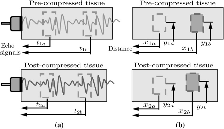
To overcome the limitations without significant improvement of the hardware system, it is essential to employ an efficient strain estimation method that requires minimal computational resources while providing high quality elastography. Many strain estimation methods for elastograhpy have been proposed to assess the map of strain distribution induced by externally or internally applied loading; they can be classified into three main categories: time-domain-based, spatial-domain-based and phase-based. Time-domain-based strain estimation methods such as time-delay strain estimation (TSE) [1] estimate the displacement using the time delays between two data sets acquired at different time points. Strains are calculated from the time delay generally obtained by cross-correlation of pre- and post-compression radiofrequency (RF) echo signals (Fig. 1a), i.e.
| 1 |
where and are the arrival times of the pre-compression echoes from the two reference windows (proximal and distal), respectively, and and are the arrival times of the post-compression echoes from the same windows, respectively.
Fig. 1.
Principles of conventional strain estimation methods: a time-delay strain estimation (TSE) and b displacement-gradient strain estimation (DSE)
Space-domain-based strain estimation methods such as displacement-gradient strain estimator (DSE) [5, 6] directly estimate the displacement in compressed region using digital image correlation (DIC) technique which measures the degree of deformation by comparing two ultrasound B-mode images of the same region acquired at two different stages, i.e. pre- and post-compression. Strains are estimated by taking the gradients of the displacements (Fig. 1b):
| 2 |
where and are the coordinates of the proximal and distal windows in the pre-compression image, respectively, and and are the coordinates of the same windows in the post-compression image, respectively.
In phase-based strain estimation (PSE) methods, the strain can be obtained from the measure of strain rate acquired by Doppler tissue imaging techniques, as temporal integration of the strain rate is equivalent to the spatial derivative of the velocity [13]. Depending on the velocity measures at each point in the region of interest, the amount of the deformation of tissues and the speed of the deformation caused by an applied external compression can be estimated. Typically, the axial differentiation of velocity field is calculated by autocorrelation algorithm [14] based on the assumption that the speed of sound c, sampling frequency , and the pulse repetition period are the known constants. Then, strains can be defined as
| 3 |
However, in portable ultrasound, the pulse repetition period is equivalent to the data dumping interval via Wi-Fi network, which varies significantly depending on the size of dataset and/or CPU load; thus it cannot be regarded as constant. Furthermore, the speed of sound varies depending on the acoustic impedance of tissues. Therefore, although PSE is computationally very efficient, it cannot be adopted for portable ultrasound in its current form.
In this study, we propose a new strain estimation method, called the robust phase-based strain estimation (RPSE), which is robust to the variations ultrasound parameters such as the speed of sound, sampling interval and pulse repetition period, thus can overcome the limitations of portable ultrasound devices in implementing elastography function. Furthermore, the RPSE algorithm is computationally very efficient, so it can be operated in wireless-connected mobile device or laptop computer without adding much computational burden. For the validation of the proposed method, the quality of the elastograms produced by RPSE are evaluated and compared with those by other strain estimation methods by means of image quality measures and computation speed.
Robust phase-based strain estimation
Velocity estimation
The fundamental Doppler equation expresses the frequency shift (Doppler frequency) of acoustic energy scattered from a target moving at some velocity in terms of the frequency of the incident wave , the speed of sound c in the propagation medium, and the angle between the direction of motion and the direction of sound propagation as
| 4 |
This implies that the Doppler frequency carries information about the axial velocity of the moving reflector. If the axial velocity is sufficiently slower than the speed of sound c, the axial velocity can be obtained as
| 5 |
In the practice for elastography, the wave direction is usually identical to the moving direction, so can be regarded as zero. Therefore, the axial velocity can be estimated by determining only the Doppler frequency , assuming that c and are known and constant. Since this conventional Doppler method uses information from a relatively narrow band of frequencies to measure the phase changes in the carrier frequency, it is also called narrowband Doppler.
1D autocorrelation
In 1985, Barber et al. [15] proposed a phase-coherent Doppler velocity estimator based on 1D autocorrelation. This method estimates the mean Doppler frequency by measuring I and Q components of the reflected pulsed signals at different time frame (slow-time axis), i.e.
| 6 |
where is the autocorrelation function of the RF signals at lags in slow-time axis, is pulse repetition period (slow-time sampling rate), and is the phase of . By combining (5) and (6), the axial velocity is obtained as
| 7 |
Using the velocity difference between two reference points, strain between the points can be calculated (Eq. 3). High computational efficiency of 1D autocorrelation algorithm has made this a suitable algorithm for real-time elastography. However, due to stochastic nature of the RF signal and the variations of c and , derived usually exhibits large fluctuations [16].
2D autocorrelation
To reduce the variance of the velocity estimates, Wilson [17] proposed broadband pulsed Doppler based on 2D fast Fourier transform by considering RF data as a 2D function of depth and time. He showed that the 2D FFT of RF data from a moving target forms a line whose slope is proportional to the target velocity. Loupas et al. [18] extended Wilson’s work to discrete limited-duration signals by examining the case of an ideal point target. They showed that 2D spectrum of a discrete version of backscattered RF signal is zero apart from a line passing though the origin of the 2D frequency plane with a slope equal to
| 8 |
which is in principle the same as conventional narrowband Doppler equation. Equation (8) also implies that although mean RF center frequency may fluctuate randomly, corresponding mean Doppler frequency tracks these fluctuations so that their ratio is always constant and proportional to the mean axial velocity. The center frequency can be estimated using the autocorrelation of the signal in the depth direction (fast-time axis) as
| 9 |
where is the sampling interval (fast-time sampling rate).
By combining Eqs. (6), (8) and (9), the mean velocity evaluated by 2D autocorrelator can be expressed as
| 10 |
where . Since Eq. (10) does not include center frequency term anymore, the velocity estimated by 2D autocorrelation shows much less fluctuation than the one by 1D autocorrelation (Eq. 7); however, it is still a function of the sampling rate and the pulse repetition period (sampling interval between frames) . In portable ultrasound, is equivalent to data-dumping interval via Wi-Fi network that cannot be constant, but varies with RF data file size and wireless communication environment. Therefore, the 2D autocorrelation cannot be directly applied to the elastography for portable ultrasound.
Strain estimation using 2D autocorrelation
The axial strain of a segment that has been deformed along loading direction is defined as
| 11 |
where is the difference between the final length L and initial length of the segment.
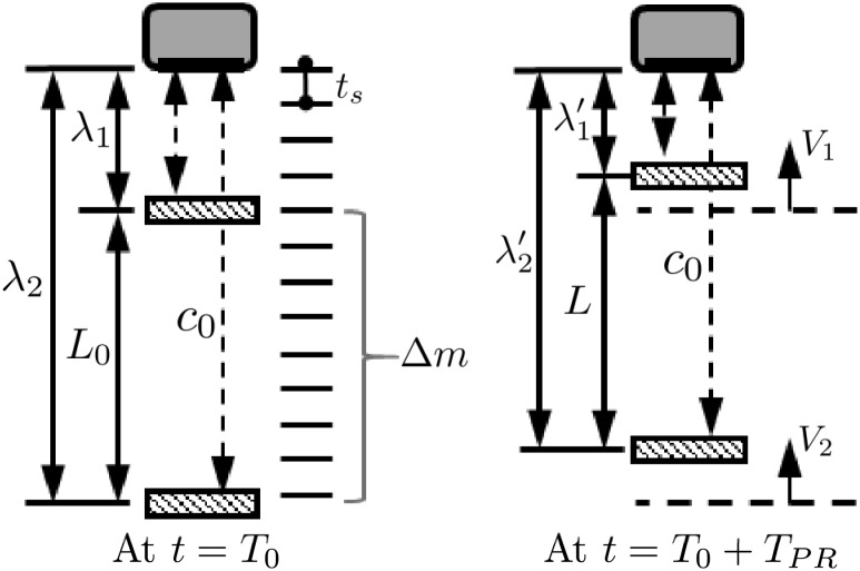
In elastography, it can be assumed that an ultrasonic transducer transmits waves toward an object moving with an instantaneous velocity V as depicted in Fig. 2. If a segment is defined as the region of axial length L 0, and the upper and the lower endpoints of the segment are away from the transducer by the distance λ 1 and λ 2, respectively (Fig. 2), the echo delays from the upper and the lower endpoints at time are
| 12 |
respectively. Since and , the axial strain can be written with echo delays by combining Eqs. (11) and (12) as
| 13 |
The change in the length of the segment , so the echo delay is related to the velocity as
| 14 |
By substituting Eq. (14) into Eq. (13), the speed of sound c is canceled and the axial strain can be rewritten as
| 15 |
Now let’s consider an axial segment along single scan line. If the segment is centered at m depth samples with the upper and lower endpoints given by and , the axial length of the segment is
| 16 |
where the tunable parameter controls the length of the axial length of the segment. By substituting Eq. (16) into (15) and rewriting and using Eq. (10), the local axial strain can be rewritten as
| 17 |
that can be further simplified as
| 18 |
where and are the 2D autocorrelation values at both endpoints of the segment.
Fig. 2.
Principle of RPSE: ultrasonic transducer transmits waves toward a segment (left). The lower (farthest away from the transducer) and upper endpoints of the segment are moving with an instantaneous velocity and , respectively (right). As a result, the segment length L 0 at is changed to L at
Note that Eq. (18) contains only segment length and the phase angle Γ at the upper and lower end points of the segment, and is not affected by sampling intervals along depth (T s) and frame (). Therefore, although data dumping interval is not consistent in portable ultrasound, strain estimation accuracy is not degraded, which makes the proposed RPSE method as a feasible strain estimator for the elastography in portable ultrasound.
Least-squares strain estimation
The local axial strain estimator in Eq. (18) only uses the autocorrelation samples at the endpoints and , which can cause strain estimate very sensitive to signal noise. Assuming that the 2D autocorrelator in Eq. (10) is linear along the depth within the segment, where the segment is centered at depth , then the autocorrelation relationship can be rewritten as
| 19 |
where the index is a natural number restricted by The relationship can be rewritten by the matrix form as . In case only the inaccurate (noisy) measured vector is known and the true vector is unknown, the sum of the squared error between the linear model and the measured autocorrelation is minimized by the least-squares method, and the minimized can be regarded as the axial strain.
Elastographic processing
Strain estimators generally compute the average strain experienced over the small time-period. When the strains are generated by periodic forces, the frame-to-frame strain values are not only changed periodically but also contaminated with significant noise, so the strain images are too crude to illustrate the relative stiffness in elastogram. In order to improve the contrast of relative stiffness of the regions, an elastographic post processing has been developed [14] by combining statistical thresholding and data smoothing. In this study, the mean (μ) and the standard deviation (σ) of a strain image are calculated and the strain magnitudes are thresholded to the range . Afterward, median filter is applied for data smoothing, i.e. a grey value of a pixel is replaced with the median of m by n matrix around the pixel to reduce the local noise and to improve the visual appearance of the elastographic images.
Methods
This section describes the numerical simulation and experimental methods to validate the performance of RPSE method.
Numerical phantom data sets
A numerical phantom of the size mm with a stiff cylindrical inclusion (10 mm) in a soft matrix was modeled using commercial finite element analysis (FEA) code (Abaqus/CAE 6.10) (Fig. 3, left). The FEA model was meshed with approximately 427,000 3D quadratic tetrahedron elements and 77,000 nodes. The elastic modulus of the matrix and the inclusion was set to 20 kPa and 100 kPa, respectively, mimicking a carcinoma in a breast tissue. Poisson’s ratio of 0.49 was applied to the whole phantom. The movement in the vertical direction at the bottom of the phantom was constrained while 0.1% axial compressive strain was applied to the top surface. We selected 0.1% compression [0.05 mm, 0.11 λ (wavelength)] because it is within the correlation range of all strain estimators. The coordinate of each node was saved to generate the deformation field data sets.
Fig. 3.
Numerical phantom modeled by FEA and Field II code
Field II code [19, 20], a Matlab-based ultrasound simulation code, was used to add random scatters to the nodal displacements and generate the corresponding pre- and post-deformation RF signal data from the numerical phantom (Fig. 3, center). The amplitudes of the random scatters were kept constant throughout the phantom; thus the inclusion could not be detected in the RF signal or B-mode image. In order to simulate both the conventional and the portable ultrasound devices, two kinds of linear probe were virtually modeled by Field II. The first one was modeled to have 192 ultrasound elements and 64 active elements to mimic conventional ultrasound device, while the other had 152 and 24 elements simulating portable ultrasound device. The numerical data sets acquired by these virtual probes are called NP-64 and NP-24, respectively, in the rest of the paper. Other acoustic parameters were set to the same values in both phantoms: the center frequency of the transducer was placed at 3.5 MHz and the sampling rate of RF signals was set to 28 MHz. The speed of sound through the phantom was set to 1540 m/s. In this setting, Field II generated 128 simulated RF lines (A-lines) and each RF line contained 2589 samples for the phantom depth. Acoustic parameters used in the numerical phantoms are listed in Table 2.
Table 2.
Acoustic parameters for numerical phantoms
| NP-64 | NP-24 | |
|---|---|---|
| Phantom size (mm3) | 40 × 50 × 10 | 40 × 50 × 10 |
| Center frequency (MHz) | 3.5 | 3.5 |
| Sampling frequency (MHz) | 28 | 28 |
| Width (mm) | 0.44 | 0.44 |
| Height (mm) | 5 | 5 |
| Kerf (mm) | 0.022 | 0.022 |
| Number of elements | 192 | 152 |
| Tx elements | 64 | 24 |
| Rx signals considered | 128 | 128 |
| Tx/Rx focus (mm) | 50 | 50 |
Various strain estimation methods (RPSE, TSE, PSE and DSE) were applied to the simulated RF data sets to estimate the strain fields (Fig. 3, right). The differences between the strain estimates and the true strains computed by the FEA were regarded as estimation errors.
Gelatin-based phantom data set
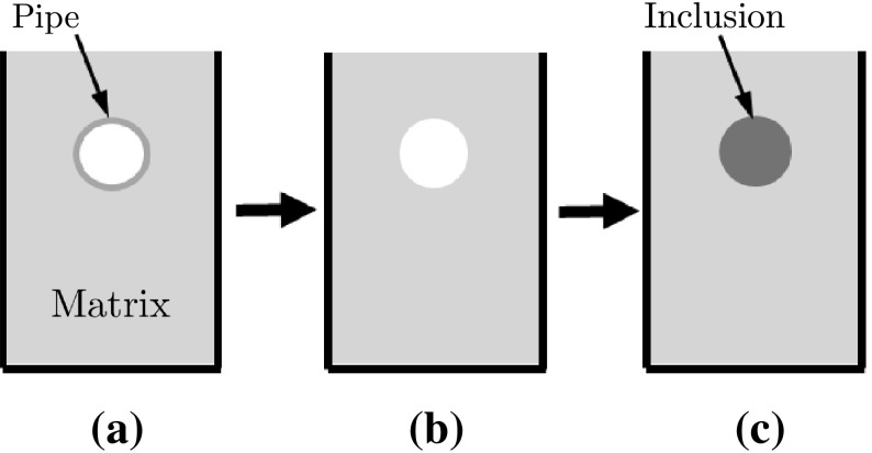
A gelatin-based phantom containing a stiffer cylindrical inclusion was designed to mimic a carcinoma in a normal tissue [5]. Following the protocol in Madsen et al. [21], the inclusion and the matrix were made with the same constituents to have the similar echogenicity (Fig. 4). The fabricated phantom contained a cylindrical inclusion (12 mm diameter) five times stiffer than surrounding matrix (47 ± 2 vs. 9 ± 1 kPa).
Fig. 4.
Schematic of phantom fabrication procedure: a 5% gelatin solution is poured into the mold with the pipe insert; b After gelatin is set, one side plate of mold and the insert are taken out; and c 20% gelatin solution is poured into the empty hole to form the inclusion
A commercial portable ultrasound scanner, Sonon 300C (Healcerion Ltd., Korea) with wireless connectivity via Wi-Fi IEEE 802.11 b/g/n, was used for the experiment on the gelatin phantom. SononPlayer, the debugging software for developers, provided the functions to record and export RF data of each ultrasound frame to personal labtop computer for post-processing. Each recording consisted of 128 channels RF data (A-lines), acquired using a 3.5 MHz convex probe with sampling frequency of 28 MHz.
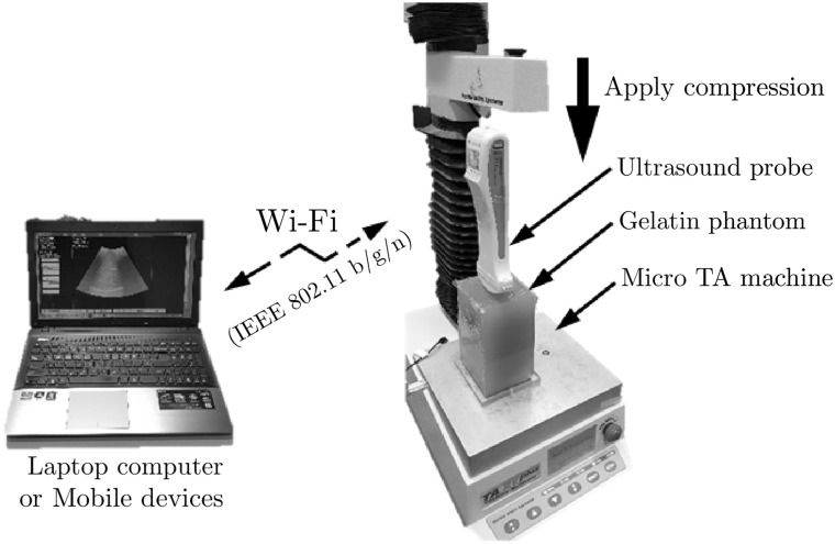
Ultrasound RF data were acquired while the phantom was being compressed with a portable ultrasound probe fixed to a TA micro test machine (TA.xt Plus, Stable Micro Systems Ltd, UK) with a 5 kgf load cell (Fig. 5). The portable ultrasound probe was connected to the personal computer via wireless connection. For the data acquisition, the portable ultrasound probe was moved downward to pre-compression position at which the curved probe perfectly touched the surface of the phantom. Then the probe was moved downward stepwise with the displacement at each step corresponding to 0.1% strain increase in the phantom. An ultrasound frame was recorded in the computer via wireless communication at each step. 0.1% strain (equivalent to 0.130 mm displacement) was chosen as a step size, because the corresponding phase change [0.29 (wavelength)] was within the detectable limit of PSE and RPSE (0.5). This was repeated until 1% compressive strain was reached in the phantom (total 11 frames).
Fig. 5.
Experiment setup for the elastographic phantom test using portable ultrasound
Implementation of strain estimators
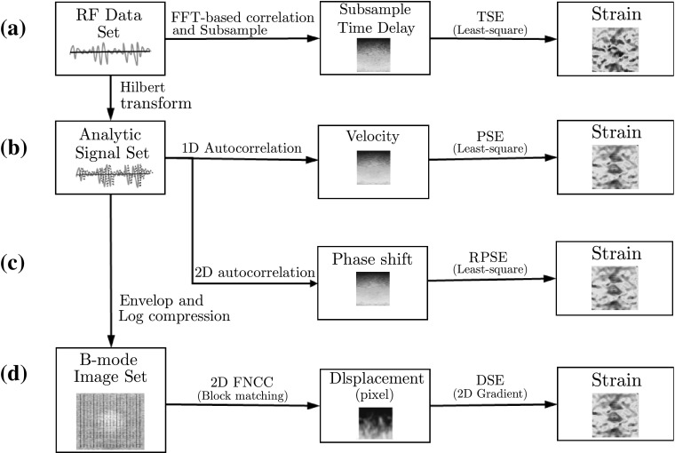
TSE, PSE, RPSE and DSE were implemented using MATLAB (The MathWork Inc., MA, USA) as conceptually illustrated in Fig. 6. The algorithms for each strain estimator are briefly described in this section.
Fig. 6.
Flow chart of strain estimators: a time-based strain estimator (TSE), b phase-based strain estimator (PSE) c robust phase-based strain estimator (RPSE), and d displacement-based strain estimator (DSE)
TSE [1] was based on the time delay of raw RF signals (Fig. 6a), which was found by the correlation function as the peak of correlation between the pre- and post-compression signals. Since FFT-based correlation is significantly faster and is also equivalent to linear convolution, it was selected as the TSE algorithm. Window size for correlation was chosen to be 45 samples (1.237 mm) for all data sets. In addition, subsample algorithm was implemented to enhance the estimation accuracy by adopting cosine fitting method using 3 points adjacent maximum correlation point. Least-squares strain estimation was also employed to compute the strain distribution that is the slope of fitted displacement curve.
For implementing PSE and RPSE, phase delay between a pair of ultrasound analytic signals formed with the RF data and its Hilbert transform was first estimated (Fig. 6b, c). Since each data frame of both numerical and gelatin phantom data sets was acquired from time-independent systems (data was dumped at each displacement), pulse repetition period () cannot be assigned as a constant value; thus the conventional PSE method can not be implemented. For the comparison with other strain estimators, pulse repetition periods of gelatin and numerical phantom were set to 11, 4 s, respectively, which produced the similar scale of strain values to other methods. In RPSE (Fig. 6c), strains were directly estimated using 2D autocorrelation (Eq. 15). Phase unwrap function in MATLAB was performed to expand the phase limit of PSE and RPSE up to a half wavelength (0.5 ) by preventing aliasing. Least-square method was also utilized to compute the curve-fitted slope of phase delay and the corresponding strain distribution.
Since DSE directly estimates displacement distribution from spatial domain, the raw RF data should be converted to B-mode image using Hilbert transform and log-compression (Fig. 6d). In addition, bi-interpolation was conducted to increase data resolution of B-mode image because sampling interval in the axial direction is significantly higher than that in the lateral direction (typically more than 10 times) [22]. A block matching algorithm based on 2D fast normalized cross-correlation (FNCC) calculated the displacements of the selected grids in a pair of pre- and post- compression B-mode images. 2D subsample method using a second order polynomial equation was used to enhance the accuracy of the displacement estimate. Then the strain distributions can be estimated by finding the 2D gradient function from the displacement field. The detailed block matching algorithm used in this study is provided in the Ref. [5]. The distances between grid points in both lateral and axial directions were set to 15 and 60 pixels, respectively, considering computation efficiency and image resolution. The side lengths of squared blocks centered at grid points for both the pre- and post-compression B-mode images were 45 and 68 pixels, respectively.
Image quality measures
Strain errors were quantified using signal-to-noise ratio (SNRe) and contrast-to-noise ratio (CNRe) that were employed as metrics for the quality of the elastograms. The elastographic SNRe identifies the quantitative measurement of the accuracy and precision of the elastograms, and is defined as [23]
| 20 |
where is the mean value of the strain, and is the standard deviation of the measured strain. The elastographic CNRe is an important parameter to determine the detectability of a stiff lesion in elastograms and is defined as [24]
| 21 |
where and are the mean and the variance values for the inside (subscript ) and the outside (subscript ) of the lesion, respectively.
Results and discussion
RPSE, TSE, DSE and PSE were applied to the numerical data sets acquired from the numerical phantoms with virtual probes and the experimental data sets from the gelatin phantom with the portable ultrasound device. Virtual probes with 24 and 64 active elements were used to simulate portable ultrasound device and conventional one, respectively. Displacement field and elastogram produced by each estimator were investigated to evaluate their estimation accuracy. Computational efficiency was also assessed by measuring the computation time spent by each algorithm to generate elastograms.
Displacement estimation
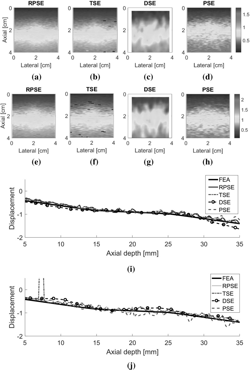
The displacement fields for two types of numerical data sets (NP-64 and NP-24) estimated by RPSE, TSE, DSE and PSE are presented in Fig. 7. The velocity fields by PSE are scaled to match with displacement fields from the other methods. Although the fields generated by RPSE (Fig. 7a, e), TSE (Fig. 7b, f) and PSE (Fig. 7d, h) look similar, the RPSE shows more delicate and smoother patterns with less decorrelation errors than the others. On the other hand, DSE (Fig. 7c, g) cannot generate the right pattern and the field around the circular inclusion is significantly mingled. No significant differences are found between the displacement fields for NP-64 (virtually acquired by conventional ultrasound) and NP-24 (portable ultrasound), but the ones for NP-24 (Fig. 7e–h) show slightly lower resolutions and more decorrelation errors than those for NP-64 (Fig. 7a–d), due to less number of active elements and lower lateral resolutions. The above results can be quantitatively represented using the displacement plots measured along the vertical centerline across the displacement fields (Fig. 7i, j). Note that the FEA plot was formed using the noiseless data from FEA, while the other plots were produced from the data in which slight random noises were introduced by Field II. RPSE, TSE and PSE plots show relatively good agreement with the FEA plot, with slight variations caused by the random noises. The DSE plot presents the smoothest trend; however, it is deviated from the FEA plot in some regions. The displacement plots for NP-64 (Fig. 7i) and NP-24 (Fig. 7j) show similar trends over all, although slightly higher levels of deviations are observed in NP-24 plot.
Fig. 7.
Displacement fields of NP-64 numerical phantom estimated by: a RPSE, b TSE, c DSE, and d PSE; displacement fields of NP-24 estimated by e RPSE, f TSE, g DSE and h PSE; displacement plots along the vertical centerline of i NP-64 and j NP-24 estimated by FEA, RPSE, TSE, DSE and PSE, respectively
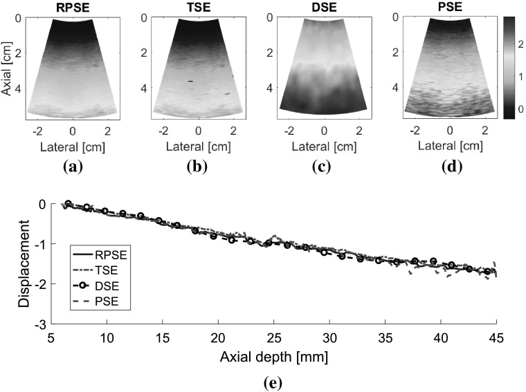
The displacement fields for the gelatin phantom were also analyzed (Fig. 8). Since the experimental data contained higher level of signal noises than the numerical data, the estimated displacement fields are generally nosier and coarser than those of numerical phantom. The displacement field generated by RPSE (Fig. 8a) shows smooth and continuous pattern and the inclusion in the center is discernable with smaller displacement than the surrounding matrix at the same depth. Both TSE and PSE displacement fields (Fig. 8b, d) poses similar behavior to RPSE field, but much noisier patterns are observed. A short black line in the middle of the image indicates a spot where decorrelation occurs. The result from DSE (Fig. 8c) shows blurred and mingled pattern, especially in the soft matrix region under the inclusion. The above behaviors are also demonstrated by the displacement plots in Fig. 8e where RPSE and TSE generate similar plots except a local peak around the middle of the depth in TSE. DSE plot is the smoothest, but slightly deviates from the others in some regions, which is consistent with the trends observed in Fig. 7. The displacement plot for PSE converted from velocity shows much higher variations than the others, particularly after 35 mm depth.
Fig. 8.
Displacement field of the gelatin phantom estimated by: a RPSE, b TSE, c DSE and d PSE, and e the displacement plots along the vertical centerline from RPSE, TSE, DSE and PSE
Elastograms
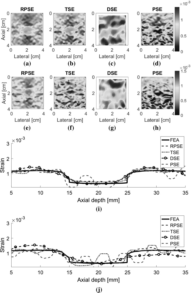
Elastograms depicting the axial strain fields generated by different strain estimators were presented in Fig. 9. The elastograms generated by RPSE (Fig. 9a, e) successfully describe the shape of the inclusion as a low strain region in the center. Furthermore, the strains inside the inclusion and in the outer matrix are almost constant, respectively, which is in accordance with the FEA result. The elastogram of NP-64 seems more delicate and smoother, but the one of NP-24 also demonstrates clearly discernable patterns. In TSE elastograms (Fig. 9b, f), the inclusion is readily detectable; however, the shape of the inclusion is distorted and the matrix strain is inconsistent and noisy. The elastogram of NP-64 (Fig. 9b) shows reasonably preserved pattern, but that of NP-24 (Fig. 9f) is much more degraded, particularly in matrix region. In DSE elastograms (Fig. 9c, g), low strain region corresponding to the inclusion is observed in the center, but the patterns are significantly dispersed and degraded. PSE elastograms (Fig. 9d, h) also show the existence of the inclusion; however, the shape of the inclusion and the matrix strain are much more distorted and noisier than RPSE.
Fig. 9.
Elastograms of NP-64 numerical phantom generated by: a RPSE, b TSE, c DSE and d PSE; elastograms of NP-24 generated by: e RPSE, f TSE, g DSE and h PSE; the strain plots along the vertical centerline of i NP-64 and j NP-24, estimated by FEA, RPSE, TSE, DSE and PSE, respectively
Strain plots along the vertical centerline of numerical phantoms (Fig. 9i, j) show the comparison between the FEA results and those from strain estimators. For NP-64 (Fig. 9i), both RPSE and TSE plots show good agreement with the FEA plot, and clearly indicate the existence of stiff inclusion in the depth between 15 and 25 mm. DSE plot is over-smoothed, and the shape and size of the inclusion are hard to be identified. PSE plot shows similar trend to FEA plot, however, it varies significantly within the inclusion and in the matrix, particularly in the deep region between 30 mm and 35 mm depth. In the strain plots of NP-24 (Fig. 9j), the plots from strain estimators present generally large deviations from the FEA plot; RPSE plot still follows the true strain relatively well, while large differences are found in TSE plot, particularly in the matrix region under the inclusion. Over-smoothing is observed in DSE plot, with much more serious manner than for that in Fig. 9i, while PSE shows very noisy and degraded results.
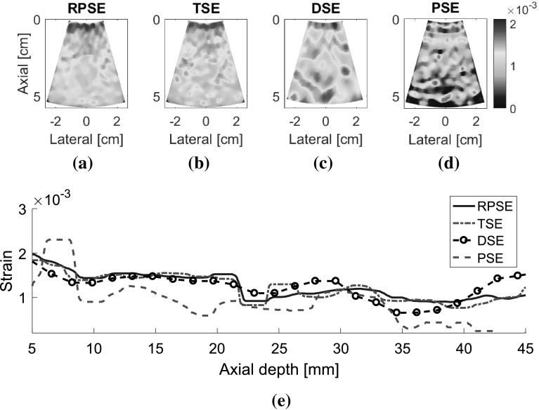
As for the elastograms of gelatin phantom, RPSE (Fig. 10a) describes the shape of the inclusion relatively well. TSE also indicates the existence of the inclusion; however, the strain patterns are highly noisy and scattered both in the inclusion and in the surrounding matrix. In the DSE elastogram (Fig. 10c), the shape of the inclusion is unclear and dispersed; furthermore, there are many degraded spots in the surrounding matrix. The elastogram from PSE (Fig. 10d) fails to describe the inclusion and only shows highly noisy pattern. In the strain plots along the vertical centerline (Fig. 10e), the strain levels inside the inclusion and the matrix are supposed to be constant, respectively; however, both RPSE and TSE plots show significant variations. Since both plots present similar trends, there is a possibility that gelatin phantom was not cured uniformly and material properties were not homogenous. Meanwhile, DSE plot shows significant variations in an over-smoothed manner compared to the other plots. PSE plot seems to deviate from the trend of the other plots across the entire depth.
Fig. 10.
Elastograms of the gelatin phantom generated by: a RPSE, b TSE, c DSE and d PSE; e the strain plots along the vertical centerline estimated by RPSE, TSE, DSE and PSE
Image quality measures
Two image quality measures, SNRe and CNRe, were evaluated over 11 frames of elastograms produced by RPSE, TSE, DSE and PSE, as presented in Fig. 11 using box plots. Note that the width of the band plots along vertical direction represents the dispersion of the measures over the frames. For the elastograms of NP-64 numerical phantom (Fig. 11a), SNRe plot associated with the RPSE elastograms yields the highest median of 6.15, but the dispersion is relatively large. The SNRe plot for TSE forms very narrow band with the medians of 4.93, while that of DSE is slightly more dispersed and the median is around 3.1. The lowest SNRe is delivered by PSE at around 2.5. As for CNRe plots, RPSE produces the highest median of 53.52 dB followed by TSE (45.33 dB), PSE (34.87 dB) and DSE (30.1 dB). The widths of the CNRe bands for RPSE, PSE and DSE are approximately the same, while that of TSE is widely dispersed. Overall, RPSE shows the best SNRe and CNRe combination with the highest median, while the repeatability over 11 frames is approximately the same.
Fig. 11.
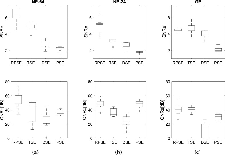
SNRe and CNRe for the elastograms of: a NP-64, b NP-24, and c the gelatin phantoms
For the elastograms of NP-24 (Fig. 11b), the SNRe for RPSE also shows the highest median at around 5.22 followed by TSE (3.27), DSE (2.74), and PSE (1.81). The width of SNRe band is the narrowest for both RPSE and PSE and becomes wider in the order of TSE and DSE. As for CNRe, PSE yields slightly higher median at around 49.14 than RPSE (47.62 dB), followed by TSE (33.03 dB) and DSE (23.07 dB). In regard to the dispersion of CNRe, RPSE shows the narrowest level and the others are almost same.
For the elastograms of gelatin phantom (Fig. 11c), the SNRe for TSE shows slightly higher median at around 4.61 than RPSE (4.39); however, its dispersion is larger than that for RPSE. PSE produces the lowest SNRe (1.98) and DSE (3.88) shows the largest dispersion. As for CNRe, both RPSE and TSE produce similar medians at around 40.65 and 40.44 dB, respectively, with almost equivalent band width. PSE produces slightly lower CNRe (30.43 dB), while DSE is associated with the lowest median (16.77 dB) and much wider band width. Overall, both RPSE and TSE show similar level of image qualities while RPSE demonstrates slightly better repeatability.
In conclusion, the results of image quality measures suggest that RPSE produces the best elastogram from the numerical data sets; however, for the experimental data set from gelatin phantom containing relatively high level of noise, RPSE and TSE shows similar performance, while PSE and DSE produces much lower SNRe and CNRe in all cases.
Computational efficiency
Since the correlation function for strain estimation imposes high computational load while portable ultrasound device has limited resources, computational efficiency is one of the critical factors in assessing the strain estimators for portable ultrasound. Computation times were measured on a Windows 7 computer (2.3 GHz, i7-3610 CPU with 12 GB RAM, ASUS-K55VD) using in-house developed Matlab code.
Figure 12 presents the computational times for the strain estimators to generate elastograms from numerical and gelatin phantom data sets. Overall, both phase-based strain estimation methods (RPSE and PSE) delivered much higher computational efficiency than correlation-based methods (TSE and DSE) by a significant margin. In order to perform the calculations for the strain estimation over 11 frames from NP-64 numerical data set of the size 1600 (length) × (scanline) per each frame (Fig. 12a), RPSE and PSE spent only 0.64 and 0.53 s, respectively, while 65.95 and 77.92 s were taken by TSE and DSE, respectively. For each RF frame, RPSE and PSE recorded only 0.06 and 0.05 s computation times, while TSE and DSE spent around 6 and 8 s. Similar amount of computation times were required for the elastogram from NP-24 phantom (Fig. 12b) by each method, with RPSE and PSE taking much less time (around 0.6 s) than TSE and DSE (63.57 and 85.56 s, respectively). The computations of each frame were 0.06, 0.05, 5.78, and 7.78 s by RPSE, PSE, TSE, and DSE, respectively.
Fig. 12.
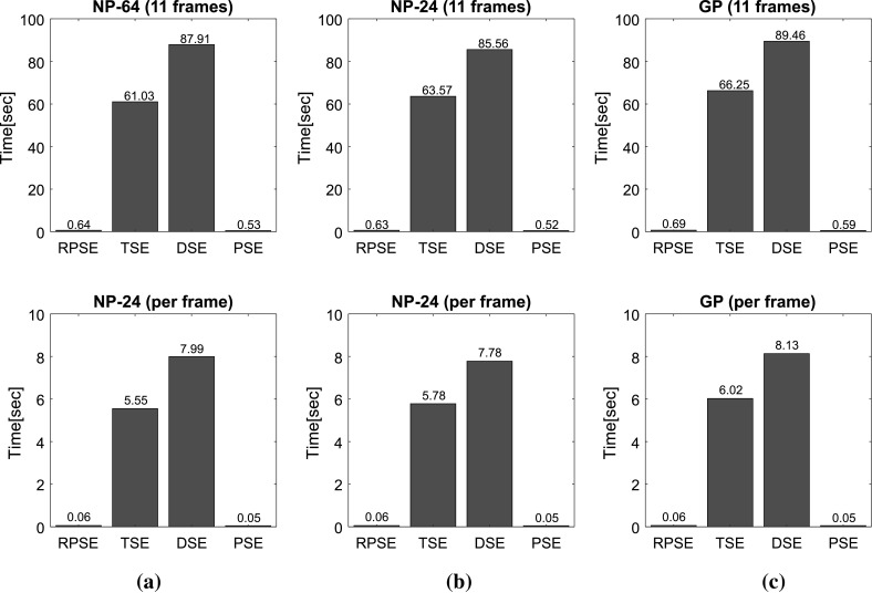
Computational times spent by RPSE, TSE, DSE and PSE methods for generating the elastogram(s) of: a NP-64 numerical phantom, b NP-24 numerical phantom, and c the gelatin phantom
The gelatin phantom data set is composed of 11 frames with each frame size of 2000 (length) × 66 (scanline). The computation of the whole frames took only 0.69 s for RPSE and 0.59 s for PSE, while TSE and DSE recorded 66.25 and 99.46 s, respectively. Both RPSE and PSE also show almost 100 times faster computational performance than TSE and DSE in the strain estimation of each frame (0.05–0.06 vs. 6.3–7.68 s). Computation time for each frame using RPSE can be converted to 16.6 fps (frame per second), that can be regarded as quasi-real-time processing. This implies that RPSE, without using C programming and MEX interface in Matlab, may be an efficient strain estimation algorithm for portable ultrasound, and although not as fast as high-end console style ultrasound device implemented with dedicated hardware (around 30 fps), RPSE running on a general personal computer have the potential to provide near-real-time elastography.
Comparison of the strain estimators
Strengths and weaknesses of each strain estimator identified through the above evaluation processes can be summarized as below. The strengths of RPSE lie in good accuracy of elastogram, high computational efficiency, and easy parameter setting. As discussed above, RPSE demonstrated the best image quality measures for numerical phantoms and the faster computation speed than those of both TSE and DSE. Moreover, parameter setting for RPSE is straightforward because it directly estimates the displacement from the phase delay between a pair of RF data sets, and does not require any searching process. On the other hand, RPSE has the phase limitation that it cannot estimate the displacement larger than a half ultrasound wavelength. However when the frame rate of ultrasound devices is over 15 fps, the displacement between consecutive frames in elastography practice is mostly within this limitation. Therefore, the phase limitation of RPSE is not a significant concern to implement the elastography in the portable US device. However, if the frame rate is very low, or the movement of the target object is fast, this can cause a problem.
The strengths of TSE are decent accuracy of elastogram and the robustness in estimating the large displacement. Unlike the RPSE with phase limitation, TSE does not have the displacement limitation because the correlation function finds the maximum correlation value throughout the searching region of which the size can be easily adjusted to increase the measurement range. However, due to the correlation algorithm involving intensive computation, TSE requires higher computational cost and more sensitive parameter settings than those for RPSE.
The benefit of DSE is that it uses B-mode images, and does not require raw RF data sets. Since most of commercial US scanners provide B-mode images, DSE can be an affordable option to generate the elastograms from various types of medical imaging modalities. However, the accuracy of DSE is relatively low and the computational cost is extremely high due to its 2D block matching algorithm. Also, the parameter settings in DSE for its 2D correlation is very sensitive and requires multiple empirical trials to obtain acceptable quality elastogram images.
The PSE demonstrates the best computational efficiency among all methods tested. However PSE delivers the highest error levels (lowest SNRe values) because it is sensitive to the variation of acoustic parameters. Moreover, PSE cannot be directly applied to the current portable ultrasound device, because pulse repetition period, an essential parameter for velocity estimation, is not constant, but varies with data size and communication environment.
Conclusion
In order to overcome the limited computational performance of portable ultrasound device in realizing elastography function, we proposed a robust phase-based strain estimator (RPSE) that is independent of the speed of sound, sampling frequency and pulse repetition period. Thorough the comparative study with other representative strain estimation methods including time-delay and displacement-gradient strain estimators, it was found that the RPSE method can deliver the acceptable level of elastography in terms of elastogram quality and computational efficiency. For the numerical phantom data, RPSE showed the best SNRe and CNRe values than the other methods. TSE also generated decent quality of elastograms; however, due to its high sensitivity to signal noise, estimated strain values were locally deviated from the true strains estimated by FEA. As for the experimental data set from the gelatin phantom, RPSE and TSE demonstrated similar performance, while PSE and DSE delivered much worse SNRe and CNRe levels in all cases, respectively. One of the greatest strength of RPSE lies in the computational efficiency; it demonstrated almost 100 times faster computation speed than TSE and DSE in strain estimation. Although PSE can perform the computation almost the same as or even faster than RPSE, its accuracy is much lower than RPSE. The results suggest that the RPSE be a suitable algorithm to perform real-time elastography processing for portable ultrasound. However, RPSE has the limited displacement range between the frames, corresponding to a half ultrasound wavelength; thus, it may not be an optimum strain estimator for fast-moving tissues.
Acknowledgements
The work was supported by Natural Sciences and Engineering Research Council of Canada (NSERC).
Conflict of interest
Bonghun Shin, Soo Jeon, Jeongwon Ryu, and Hyock Ju Kwon declare that they have no conflict of interest in relation to the work in this article.
Ethical approval
This article does not contain any studies with human participants or animals performed by any of the authors.
References
- 1.Ophir J, Cespedes I, Ponnekanti H, et al. Elastography: a quantitative method for imaging the elasticity of biological tissues. Ultrason Imaging. 1991;13(2):111–134. doi: 10.1177/016173469101300201. [DOI] [PubMed] [Google Scholar]
- 2.Ophir J, Srinivasan S, Righetti R, et al. Elastography: a decede of progress (2000–2010) Curr Med Imaging Rev. 2011;7(4):292–312. doi: 10.2174/157340511798038693. [DOI] [Google Scholar]
- 3.Ophir J, Alam SK, Garra BS, et al. Elastography: imaging the elastic properties of soft tissues with ultrasound. J Med Ultrason. 2002;29(4):155–171. doi: 10.1007/BF02480847. [DOI] [PubMed] [Google Scholar]
- 4.Skovoroda AR, Klishko AN, Gusakyan DA, et al. Quantitative analysis of the mechanical characteristics of pathologically changed soft biological tissues. Biophysics. 1995;40(6):1359–1364. [PubMed] [Google Scholar]
- 5.Han Y, Kim DW, Kwon HJ. Application of digital image cross-correlation and smoothing function to the diagnosis of breast cancer. J Mech Behav Biomed Mater. 2012;14:7–18. doi: 10.1016/j.jmbbm.2012.05.007. [DOI] [PubMed] [Google Scholar]
- 6.Shin B, Gopaul D, Fienberg S, Kwon HJ. Application of Eshelby’s solution to elastography for diagnosis of breast cancer. Ultrason Imaging. 2016;38(2):115–136. doi: 10.1177/0161734615573030. [DOI] [PubMed] [Google Scholar]
- 7.Lorenz A, Sommerfeld H-J, Garcia-Schürmann M, et al. A new system for the acquisition of ultrasonic multicompression strain images of the human prostate in vivo. IEEE Trans Ultrason Ferroelectr Freq Control. 1999;46(5):1147–1154. doi: 10.1109/58.796120. [DOI] [PubMed] [Google Scholar]
- 8.Rivaz H, Fleming I, Assumpcao L, et al. Ablation monitoring with elastography: 2D in vivo and 3D ex vivo studies. In: Medical image computing computer-assisted intervention—MICCAI, Berlin Heidelberg, Germany, 6 Sep 2008, pp 458–66. [DOI] [PubMed]
- 9.Chernak LA, Thelen DG. Tendon motion and strain patterns evaluated with two-dimensional ultrasound elastography. J Biomech. 2012;45(15):2618–2623. doi: 10.1016/j.jbiomech.2012.08.001. [DOI] [PMC free article] [PubMed] [Google Scholar]
- 10.Brandenburg JE, Eby SF, Song P, et al. Ultrasound elastography: the new frontier in direct measurement of muscle stiffness. Arch Phys Med Rehabil. 2014;95(11):2207–2219. doi: 10.1016/j.apmr.2014.07.007. [DOI] [PMC free article] [PubMed] [Google Scholar]
- 11.Muraki T, Ishikawa H, Morise S, Yamamoto N, et al. Ultrasound elastography-based assessment of the elasticity of the supraspinatus muscle and tendon during muscle contraction. J Shoulder Elb Surg. 2015;24(1):120–126. doi: 10.1016/j.jse.2014.04.012. [DOI] [PubMed] [Google Scholar]
- 12.Nelson BP, Sanghvi A. Out of hospital point of care ultrasound: current use models and future directions. Eur J Trauma Emerg Surg. 2016;42(2):139–150. doi: 10.1007/s00068-015-0494-z. [DOI] [PubMed] [Google Scholar]
- 13.Heimdal A, Støylen A, Torp H, Skjærpe T. Real-time strain rate imaging of the left ventricle by ultrasound. J Am Soc Echocardiogr. 1998;11(11):1013–1019. doi: 10.1016/S0894-7317(98)70151-8. [DOI] [PubMed] [Google Scholar]
- 14.Børstad TK. Intraoperative ultrasound strain imaging of brain tumors. Master Thesis, Norwegian University of Science and Technology, Norway, 2011.
- 15.Barber WD, Eberhard JW, Karr SG. A new time domain technique for velocity measurements using Doppler ultrasound. IEEE Trans Biomed Eng. 1985;3:213–229. doi: 10.1109/TBME.1985.325531. [DOI] [PubMed] [Google Scholar]
- 16.David J-Y, Jones SA. Modern spectral analysis techniques for blood flow velocity and spectral measurements with pulsed Doppler ultrasound. IEEE Trans Biomed Eng. 1991;38(6):589–596. doi: 10.1109/10.81584. [DOI] [PubMed] [Google Scholar]
- 17.Wilson LS. Description of broad-band pulsed Doppler ultrasound processing using the two-dimensional Fourier transform. Ultrason Imaging. 1991;13(4):301–305. doi: 10.1177/016173469101300401. [DOI] [PubMed] [Google Scholar]
- 18.Loupas T, Powers JT, Gill RW. An axial velocity estimator for ultrasound blood flow imaging, based on a full evaluation of the dropper equation by means of a two-dimensional autocorrelation approach. IEEE Trans Ultrason Ferroelectr Freq Control. 1995;42(4):672–688. doi: 10.1109/58.393110. [DOI] [Google Scholar]
- 19.Jensen JA, Svendsen NB. Calculation of pressure fields from arbitrarily shaped, apodized, and excited ultrasound transducers. IEEE Trans Ultrason Ferroelectr Freq Control. 1992;39(2):262–267. doi: 10.1109/58.139123. [DOI] [PubMed] [Google Scholar]
- 20.Jensen JA. Field: A program for simulating ultrasound systems. In: 10th Nordic-Baltic conference on biomed imaging. 1996, vol. 34, suppl. 1, part 1, p. 351–3.
- 21.Madsen EL, Zagzebski JA, Frank GR. An anthropomorphic ultrasound breast phantom containing intermediate-sized scatterers. Ultrason Med Biol. 1982;8:381–392. doi: 10.1016/S0301-5629(82)80006-9. [DOI] [PubMed] [Google Scholar]
- 22.Chaturvedi P, Insana MF, Hall TJ. 2-D companding for noise reduction in strain imaging. IEEE Trans Ultrason Ferroelectr Freq Control. 1998;45(1):179–191. doi: 10.1109/58.646923. [DOI] [PubMed] [Google Scholar]
- 23.Céspedes I, Ophir J. Reduction of image noise in elastography. Ultrason Imaging. 1993;15(2):89–102. doi: 10.1177/016173469301500202. [DOI] [PubMed] [Google Scholar]
- 24.Ophir J, Alam SK, Garra B, Varghese T. Elastography: ultrasonic estimation and imaging of the elastic properties of tissues. Proc Inst Mech Eng Part H J Eng Med. 1999;213(3):203–233. doi: 10.1243/0954411991534933. [DOI] [PubMed] [Google Scholar]


