Distinct Genetic Architectures for Phenotype Means and Plasticities in Zea mays

Abstract

Phenotypic plasticity describes the phenotypic variation of a trait when a genotype is exposed to different environments. Understanding the genetic control of phenotypic plasticity in crops such as maize is of paramount importance for maintaining and increasing yields in a world experiencing climate change. Here, we report the results of genome-wide association analyses of multiple phenotypes and two measures of phenotypic plasticity in the maize nested association mapping (US-NAM) population grown in multiple environments and genotyped with ~2.5 million single nucleotide polymorphisms (SNPs). We show that across all traits the candidate genes for mean phenotype values and plasticity measures form structurally and functionally distinct groups. Such independent genetic control suggests that breeders will be able to select semi-independently for mean phenotype values and plasticity, thereby generating varieties with both high mean phenotype values and levels of plasticity that are appropriate for the target performance environments.

Phenotypic plasticity describes the phenotypic variation of a trait that occurs when a genotype is exposed to different environments¹. Variation in plastic responses among genotypes is described as genotype-environment interaction (GxE)², which is an important factor in plant breeding^3,4. Understanding these interactions is important because agricultural systems will need to feed ~9 billion people by 2050, requiring a 60% increase in productivity compared to current levels⁵ while also accounting for different and increasingly variable weather patterns⁶. If plasticity is under genetic control, then genes exist that control the phenotypic mean and plastic response separately or together⁷; thus, it may be possible to breed for optimized, locally adapted cultivars that take advantage of certain environmental conditions and outperform more widely adapted cultivars⁸. Conversely, a lack of a plastic response may be better for some phenotypes such as disease resistance.

Recent studies concluded that genomic prediction for yield stability in rye⁹ and wheat¹⁰ could be effective. However, to fully exploit plasticity it is important to understand its genetic architecture. Three genetic models for the control of plasticity have been proposed. First, the overdominance model states that heterozygosity at genes causes plastic responses¹¹. Second, the allelic sensitivity model states that differentially environmentally sensitive alleles of genes that affect mean phenotypes are responsible for plastic responses^12,13. Third, the structural (or regulatory) gene model states that plastic responses are caused by the regulation of mean phenotype genes by genes that integrate environmental stimuli^14,15. Numerous studies involving modest numbers of genotypes have found evidence for both the allelic sensitivity and structural gene models to varying degrees in various organisms and phenotypes^9,16–20.

The genetic mechanism(s) responsible for plasticity has profound implications for its use in plant breeding. For example, if the allelic sensitivity model holds, breeders may need to make trade-offs between mean phenotypes and plasticity because the same genes control these properties. However, if the structural gene model holds, the selective constraint between the mean phenotype and its plasticity is at least less stringent than the allelic sensitivity model, and there is potential to exploit plastic response while also increasing mean phenotype values.

Phenotypic plasticity has not yet been studied in a large and diverse population of a single species. Maize (Zea mays ssp. mays) accounted for ~37% of worldwide cereal production in 2014²¹ and is used for human consumption, livestock feed, biofuels, and as an industrial feedstock. Maize is a diverse species with rapidly decaying linkage disequilibrium (LD) (2-10 kb)^22,23, and inbred lines can easily be replicated across locations. This makes it a useful species for association mapping and studying plasticity. In this study, we analyzed 23 agronomically relevant phenotypes and measured their plasticities on ~5,000 recombinant inbred lines (RILs) in the US nested association mapping (US-NAM) population. Using Bayesian Finlay-Wilkinson regression^24,25 and GWAS we show that the candidate genes associated with mean phenotypes and their plasticities are structurally and functionally distinct across all 23 phenotypes, suggesting that there is some flexibility in the selective constraints between a phenotype and its plasticity.

RESULTS

Variability in plasticity.

Trait values for 23 phenotypes (Supplementary Table 1) measured in 4-11 environments on the ~5,000 NAM RILs were used as inputs for Bayesian Finlay-Wilkinson regressions (FWR)^24–26 on each phenotype. FWR estimates a genotypic main effect and slope for each RIL from which a residual for each observation can be calculated and a residual variance estimated. The FWR slope measures the linear response of a RIL to the environment, relative to all other RILs in the population. A FWR slope of one denotes a RIL exhibiting the population average response to the environment, while a slope of zero denotes a RIL exhibiting no response to the environment. The residual variance for each RIL serves as a measure of model fit with larger residual variances indicating poor fits to the linear model due to environmental variables that were not modeled, non-linear responses to the environment, or lack of genetic basis for the environmental response^27,28. Genetic correlations between the mean phenotype values and plasticities for each phenotype are moderate to strong for many of the phenotypes (Supplementary Figure 1).

All 23 phenotypes demonstrated variability in linear plasticity (variances ranged from 0.021 to 0.734) and the dispersion of different phenotypes was assessed by the quartile coefficient of dispersion (QCD) (Figure 1). The ratio of two QCDs measures how dispersed two distributions are relative to each other. For example, linear plasticity for growing degree days (GDD) to flowering was more dispersed than linear plasticity for absolute time to flowering (2.66 and 1.81 times more dispersed for silking and tasseling, respectively). Because thermal time is the primary driver of development in maize²⁹ and 13/26 of the US-NAM subpopulations have a tropical parent line^23,30, we tested for an association between tropical, temperate, or mixed germplasm and dispersion in the linear plasticity of flowering time. Germplasm group was not associated with absolute days to silking or tasseling (Kruskal-Wallis test, p = 0.46 and p = 0.45, respectively), but was associated with GDD to silking and tasseling (Kruskal-Wallis test, p = 0.006 and p = 0.001, respectively) (Supplementary Figure 2). In both cases, the dispersion in tropical and temperate germplasm differed (two-sided Mann-Whitney U test, p = 0.002 for GDD to silking and p = 0.0001 for GDD to tasseling).

Figure 1.

Quartile coefficients of dispersion for the linear and non-linear plasticities of 23 phenotypes. The number of environments used to calculate plasticity is given in parentheses. See Supplementary Table 1 for the number of RILs measured for each phenotype.

Non-linear plasticities were more dispersed than linear plasticities for 22/23 phenotypes except in the case of GDD anthesis-silking interval (0.83 times as dispersed). Asynchronous male and female flowering can be adaptive in some environments³¹. Because the NAM parents were drawn from both temperate and tropical germplasm, this greater dispersion of environmental responses may reflect adaptation of the parental lines to diverse environments.

Variance explained by genome-wide SNPs.

The 2,452,207 SNPs were hierarchically assigned to six categories relative to genes using a scheme modified from Rodgers-Melnick et al.³²: exons, 5kb upstream of a gene, 5kb downstream of a gene, introns, MNase hypersensitive (HS), and intergenic regions. For example, the exon category contains SNPs found in coding sequences, and the 5kb upstream category contains SNPs found no more than 5kb upstream of the transcription start site that are also not in the coding sequence of a gene. SNPs within each category were used to construct genetic relationship matrices and the variance explained by each class was estimated for each phenotype and plasticity measure (Supplementary Figure 3). As observed by Rodgers-Melnick et al.³², variants in exons and HS regions explain the most variance for mean phenotype values (Figure 2). A similar trend was observed for the linear plasticity of the traits. The total variance explained by exonic SNPs for linear plasticities was less than that for mean phenotype values (14.6±2.8% vs. 25.3±2.3%, respectively), increasing the relative importance of regulatory variants within 5kb of genes. Very little variance was explained by genome-wide SNPs for non-linear plasticities (Supplementary Figure 3). Exonic SNPs explained a non-zero proportion of the variance in only five cases for non-linear plasticity, indicating the importance of regulatory variation in the control of this phenotypic measure.

Figure 2.

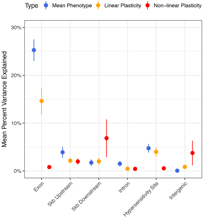
Mean percent variance explained by genome-wide SNPs hierarchically assigned to annotation categories. Error bars represent one standard error of the mean. n = 23 for each phenotypic measure and annotation category.

Genome-wide association.

Mean phenotype values and their plasticities were used as inputs for GWAS using FarmCPU³³ and 2,452,207 SNPs. SNPs exceeding a 1% FDR threshold were declared statistically significant (Supplementary Table 2; Supplementary Figure 4). This generated 977 unique SNPs that were associated with at least one mean phenotype value or plasticity measure (Supplementary Table 2). Only four SNPs were associated with more than one measure of a single phenotype. The relative proportions of significant SNPs identified for mean phenotype values and their plasticities varied across phenotypes (Figure 3a). No significant SNPs were identified for the non-linear plasticity of 2/23 (8.7%) phenotypes: ear length and leaf length. More significant SNPs were identified for the plasticities of 8/23 (34.8%) phenotypes than for the corresponding mean phenotype values. We also compared our associated SNPs to those from a traditional GWAS using the same measurements of 14 traits in US-NAM³⁴. We assumed that two SNPs tagged the same region if windows centered on each SNP overlapped and the SNPs were associated with the same phenotype. At a window size of 20 kb, 32.4% of mean phenotype and 22.2% of linear plasticity windows overlapped with a window from Wallace et al.³⁴, and all phenotypic measures had non-zero overlaps at all window sizes (Figure 3b). These overlaps were greater than expected by chance for mean phenotype values and linear plasticities at all window sizes (permutation test, p < 0.05) but not for non-linear plasticities.

Figure 3.

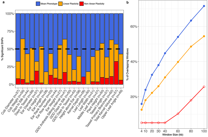
a. Relative proportions of SNPs associated with mean phenotype values and linear and non-linear plasticities for 23 phenotypes. The percentage of plasticity-associated SNPs is greater than 50% (dashed black line) for 11/23 phenotypes. b. Percentage of overlapping windows centered on associated SNPs for mean phenotype values and linear and non-linear plasticities with windows centered on SNPs from Wallace et al.³⁴. Closed circles denote windows for which more overlaps were observed than expected by chance (two-sided permutation test) at the α = 0.05 level; open circles denote windows that do not differ significantly from the null hypothesis.

Genomic distribution of significant SNPs.

We quantified the enrichment or depletion of significant SNPs in different annotation categories for mean phenotype values and linear and non-linear plasticities relative to the input distribution of SNPs. Significant SNPs for mean phenotype values were enriched for hits in exons (exact binomial test, p = 2.28×10⁻⁵) and 5kb upstream of genes (exact binomial test, p = 0.0007) and depleted for hits in intergenic regions more than 5 kb from genes (exact binomial test, p = 8.98×10⁻¹²). Significant SNPs for linear plasticities were also enriched in exons (exact binomial test, p = 0.00088) and depleted in intergenic regions (exact binomial test, p = 1.82×10⁻⁵). The genomic distribution of significant SNPs for non-linear plasticity was not significantly different from that of the input SNPs (χ² test, χ² = 7.67, df = 3, p = 0.0533).

Candidate genes for mean phenotype values and their plasticities are distinct.

Candidate genes were defined as those falling within 20kb windows centered on each significant SNP. This identified 1,158 unique candidate genes (Supplementary Table 3). More candidate genes were associated with both the mean phenotype value and linear plasticity of at least one trait than expected by chance (Fisher’s exact test, 3.07-6.83-fold enrichment, p = 4.56×10⁻¹¹) (Figure 4a). Of the 1,158 unique candidate genes only 33 (2.8%) were associated with multiple measures of at least one phenotype (Figure 4a) and of these only eight genes representing 4 windows were associated with the mean phenotype and the linear plasticity of the same phenotype. For example, two SNPs within 2.5 kb of each other tagged three genes on chromosome 2 for the mean phenotypic value and linear plasticity of total kernel volume. One of these genes (GRMZM2G372074) has rice and Arabidopsis orthologs annotated as seed storage proteins and is tagged by a SNP ~400 bp upstream of the transcription start site. The low degree of overlap between candidate genes for mean phenotype values and plasticity measures was conserved across windows of 4-100kb, where the number of overlapping genes never exceeded 1.18% of the total (Figure 4b).

Figure 4.

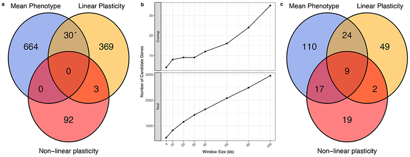
a. Number of candidate genes (n = 1,158) identified for mean phenotype values and a plasticity measure. Asterisks indicate enrichment at the α = 0.05 level (two-sided Fisher’s exact test). b. Number of overlapping candidate genes and total candidate genes at different window sizes. Total genes are those falling within a window of the given size centered on each significant SNP. Overlapping genes are those candidate genes that fall within a window for a mean phenotype value and a window for a plasticity measure of the same phenotype. c. Number of GO terms (n = 230) enriched for pools of candidate genes at a 1% FDR threshold (two-sided hypergeometric test).

Gene Ontology (GO) term enrichment.

GO enrichment analysis was performed on candidate genes across all phenotypes grouped by mean phenotype or plasticity measure using the hypergeometric test at a 1% FDR threshold. Enriched terms in this analysis indicate potential common strategies that have evolved across phenotypes for expression of the mean phenotype or responding to the environment. This identified 230 enriched GO terms in the biological process ontology (Supplementary Table 4), and only 52 (22.6%) were enriched for multiple measures of a phenotype (Figure 4c). Uniquely enriched terms for linear plasticity candidate genes included biosynthesis of hormones such as abscisic acid, maintenance of shoot apical meristem and floral organ identities, flower morphogenesis, and positive gravitropism. Surprisingly, these candidate genes were also uniquely enriched for DNA methylation, and candidate genes for both mean phenotypic value and linear plasticity were enriched for H3K9 methylation, implicating epigenetic marks in plasticity. Another notable enriched term is positive regulation of developmental heterochrony, or regulation of the rate at which developmental time points are reached. A candidate (GRMZM2G035944), associated with the linear plasticity of ear height, is annotated with this term and is a TCP family transcription factor³⁵. This family includes teosinte-branched1 and is implicated in leaf morphogenesis in maize and rice³⁶. Results for the cellular component and molecular function ontologies can be found in Supplementary Tables 5 and 6, respectively.

Protein-protein interaction networks.

We also assessed GO term enrichment for the candidate genes for each phenotype’s components and their validated and predicted interaction partners in a maize PPI network³⁷ using BiNGO³⁸ (Supplementary Tables 7, 8, and 9) and a 1% FDR threshold. This analysis provided greater insight into the different biological mechanisms by which plastic responses might influence the expression of different phenotypes. As an example, the mean total kernel volume candidate genes and their predicted interaction partners are uniquely enriched for hormone, defense molecule, and glucose biosynthesis genes. Candidates and interaction partners for the linear plasticity of total kernel volume were uniquely enriched for signaling, post-translational protein modification, and histone phosphorylation process terms. This example suggests the existence of interacting subnetworks and regulatory layers where environmental responses are integrated to affect the expression of signaling proteins and the activities of metabolic and catabolic pathways that produce a phenotype.

DISCUSSION

The genetic control of phenotypic plasticity has been variously attributed to heterozygosity at relevant genes (overdominance)¹¹, differential environmental sensitivity of alleles of a gene (allelic sensitivity)^12,13, or genes that affect the expression of the phenotype and genes that react to the environment (structural gene model)^14,15. In this study it was not possible to evaluate the extent to which overdominance contributes to phenotypic plasticity in maize because the US-NAM population is inbred. There is, however, limited evidence for a role for overdominance in the plastic response of other organisms². Furthermore, little evidence has been found for overdominance in other maize traits, e.g., grain yield heterosis³⁹. Distinguishing between the allelic sensitivity and structural gene models is a test of pleiotropy, commonly assessed by mapping two traits and comparing the similarity between their respective significant SNPs/candidate genes. We have shown that the genetic architectures underlying mean phenotype values and two measures of plasticity for 23 phenotypes map to distinct genomic regions containing functionally distinct genes in the maize US-NAM population, which strongly supports the structural gene model.

This work is conceptually similar to previous work focused on mapping genotype-specific environmental variances or variance QTLs⁴⁰. While these approaches and our approach both seek to map measures of GxE to the genome, we have focused on GxE caused by macro-environmental variation (i.e., environmental variation common to all individuals grown in a common location) while previous work has focused on that caused by micro-environmental variation (i.e., environmental variation unique to each individual)⁴⁰. Both macro- and micro-environmental variation can cause GxE but at different scales, which is likely to act through both similar and different pathways. Thus, our study is complementary to existing work on variance QTLs.

Here we have used a Bayesian formulation of the Finlay-Wilkinson model²⁵, which has allowed us to derive our estimates of the genotype-specific mean and response to the environment simultaneously. Although the prior distributions for genotype-specific intercepts and slopes are assumed independent in the Bayesian model, this does not preclude dependence in the posterior distributions.

As in other studies on phenotypic plasticity¹⁵, we observe moderate to strong genetic correlations between the mean and plasticity of most phenotypes (Supplementary Figure 1). We found only 4/977 SNPs that were significantly associated with both the mean and plasticity of the same phenotype, providing a small amount of support for the allelic sensitivity model in maize. This degree of overlap is insufficient to explain the observed genetic correlations. Co-localization of loci is the classical expectation for genetically correlated phenotypes, although it is not sufficient to prove identical genetic control. At least one genetic variant must be associated strongly enough with two different phenotypes to observe co-localization. It is possible that lack of co-localization observed in this study is the result of false negatives arising from a lack of statistical power due to small effect sizes on the two phenotypes and/or rare alleles. Such a scenario may have an outsized effect when mapping plasticity because its heritability is generally smaller than that of the mean (Supplementary Figure 3). Even if two loci co-localize, this co-localization may be a spurious result due to strong LD between multiple genetic variants⁴¹, although this scenario can only be distinguished with fine-mapping. Another possible explanation for the existence of genetic correlations in the absence of co-localization of significant loci is “mediated pleiotropy” where one phenotype lies on the causal path to another phenotype⁴¹. In this scenario we would expect to see evidence of interactions between candidate genes for the two phenotypes or their co-localization in similar pathways. We performed a non-exhaustive survey of a maize protein-protein interaction network³⁷ and found predicted interactions between some pairs of candidate genes for the mean and plasticity of the same phenotype (unpublished results), a result that is at least consistent with “mediated pleiotropy”.

Similar to the results of Li et al.⁴², we found that SNPs in exons and regulatory regions explained the largest proportions of the phenotypic variance for mean phenotype values. Our results differ from those of Rodgers-Melnick et al.³² in that we de-prioritized MNase HS regions so that they only contained putative open chromatin in intergenic regions. Using the same assignment scheme as Rodgers-Melnick et al.³², we obtained results with similar conclusions (data not shown). Genome-wide SNPs in coding sequences explained less variation in the two plasticity measures, increasing the relative importance of regulatory variation.

The genomic distributions of our associated SNPs for mean phenotype values and both plasticity measures were enriched for coding sequence and gene-proximal variation and depleted for intergenic variation similar to the results of Wallace et al.³⁴. We also observed that our mean phenotype-associated variants overlapped significantly with the trait-associated SNPs from Wallace et al.³⁴, although this overlap was less than 100%. This is likely due to the different statistical models used to calculate input phenotypes. Wallace et al. used a mixed linear model to compute RIL BLUPs, adjusting for environmental and genotype-environment interaction effects. We calculated mean phenotype values using the FWR model, which considers each RIL’s response to different environments. While these quantities are different, the amount of co-localization observed indicates that they are measuring similar genetic signals. Although the input phenotypes of Wallace et al.³⁴ are very different from our linear plasticity measure, we find significant overlaps in this comparison, indicating that the regulation of genotype-environment interactions in maize is complex.

Our candidate genes for mean phenotype values and plasticity parameters were structurally distinct for each phenotype, and this observation was consistent across varying window sizes and when using the mixed linear model (MLM) instead of FarmCPU (unpublished results). Li et al.⁴ recently mapped flowering time and its coefficient of variation (CV) in US-NAM and found that all but three QTL for flowering time CV overlapped with QTL for mean flowering time. Hence, their results support the allelic sensitivity model for the plasticity of flowering time. Although our results provide strong evidence for the structural gene model for plasticity, they also provide some evidence for the allelic sensitivity model, and it is unlikely that only one of these models explains the genetic control of plasticity. In addition to the use of different SNPs, a different GWAS model, and a different measure of plasticity (coefficient of variation), the support intervals for the QTL identified by Li et al.⁴³ are large (9.2±7.8 Mb mean±s.d.). Because these support intervals are so large, it is not possible to discount the possibility that the genes underlying them are different.

The number of candidate genes identified for either plasticity measure is relatively small compared to the number of candidate genes for mean phenotype values. There are three possible reasons for this. First, inference for statistics other than the mean often requires more data, increasing the sample size required for GWAS⁴⁴. Additionally, error propagation in the calculation of slopes and residual variances will decrease the signal-to-noise ratio, making association mapping of these measures more difficult. Increasing the number of environments in which phenotypes were evaluated would be expected to improve our power to detect plasticity loci.

Second, we have made the critical assumption that the plasticity of these phenotypes is a linear function of the environment. While this may be a good approximation for some phenotypes, it is undoubtedly not good for all phenotypes. However, precise estimation of higher order coefficients requires increasingly larger datasets. Finlay-Wilkinson regression is nevertheless a satisfactory instrument for identifying general trends in phenotypic responses across environments and has been widely used by plant breeders^26,45.

Third, while the environmental index used as an explanatory variable in the regression was calculated from the phenotypes of the genotypes grown in that environment, which is the classical index, this choice is not optimal. A better choice of environmental index would incorporate weather data for each tested environment as has been done in genomic selection^46,47. This requires not only sufficient phenotypic observations to estimate precisely additional model coefficients but also appropriate types and densities of weather data for environmental characterization. As field-based high-throughput phenotyping methods continue to be developed, development of environmental characterization methods is expected to help to fill in this gap in plasticity modeling.

Finally, we also observed that our candidate genes for mean phenotype values and plasticity measures were enriched for different GO terms. This structural and functional distinctness agrees well with our intuition that epistasis, which has proven difficult to identify via GWAS (e.g., Buckler et al.³¹), is a natural consequence of gene regulatory and biochemical networks. By separately mapping the mean phenotype value and plasticity of a single trait we can assess potential gene-gene interactions between candidate genes through analysis of protein-protein interactions, co-expression, and eQTLs.

It is important to consider not only the genetic and environmental factors influencing phenotypes, but also the gene-environment interactions that contribute to their plastic responses. We have provided evidence that the genetic architectures for mean phenotype values and plasticity are distinct and biologically complementary. While our study strongly supports the structural gene model and provides minimal support for the allelic sensitivity model, our observed genetic correlations and the results of previous mapping^16–20 and artificial selection studies^48–50 support a mixed model where phenotypic plasticity is caused by both differential expression of alleles across environments and gene-gene interactions. The plasticity of any one phenotype is likely to lie on a continuum between these two alternatives where the mixture of these two mechanisms differs by both phenotype and organism. These results can be used to explore how maize has adapted to diverse environments during its evolutionary history and under the pressure of artificial selection and to introduce genetic components into crop-growth models, allowing more accurate simulation of environmental and management decisions. While breeding for high-yielding, low plasticity cultivars is the ultimate goal of plant breeding, climate change will make the production of such cultivars more difficult as environments become more extreme and variable. Based on our results and with more detailed analysis of the interactions between specific environmental factors and genes and their effects on plasticity, it may be possible for breeders to select for cultivars that produce high yields by exploiting certain characteristics of the target performance environment.

METHODS

Phenotypes.

Values for 21 phenotypes were downloaded from Panzea (file “traitMatrix_maize282NAM_v15-130212.txt” at http://www.panzea.org/#!phenotypes/c1m50 accessed March 2015). These phenotypes were measured on the US-NAM population³⁰ planted in 2-11 environments (Supplementary Table 1). Outliers were removed as follows. First, phenotypes measured in only one or two environments were removed. Second, the interquartile ranges (IQR) were calculated for each RIL across environments and for each environment across RILs within a phenotype. Any trait measurements of RILs that were more than 1.5 times larger or smaller than either of the IQRs was removed. Finally, for a given phenotype any RIL that was not measured in at least three environments was removed. This filter removed 4-11% of available observations, leaving 16,000-44,000 observations for each phenotype (Supplementary Table 1). Two additional phenotypes, height above ear and kernel depth, were calculated using the downloaded data. Height above ear was calculated as the difference between plant height and ear height. Kernel depth was calculated as one-half the difference between ear diameter and cob diameter.

Stability analysis.

The plasticity of each phenotype was assessed using a Bayesian Finlay-Wilkinson regression (FWR) procedure implemented in the FW R package^24–26. The FW package jointly estimates the parameters of the genotype-specific Finlay-Wilkinson regression equation

$$y_i{}_j=\mu +g_i+\left(1+b_i\right)h_j+{ϵ}_i{}_j$$

where y_ij is the phenotype of the ith RIL measured in the j environment, g_i is the main effect of the ith RIL, h_j is the main effect of the jth environment, ϵ_ij is an error term assumed to be IID normal with mean zero and variance ${\sigma }_{ϵ}^2$, and (1 + b_i) is the change in expected performance of the ith RIL per unit change in the environmental effect (h_j). All parameters are treated as random effects where

$$\begin{gathered} \mathit{g}=\left\{g_i\right\}\text{~}N\left(0,\mathit{A}{\sigma }_g^2\right) \\ \mathit{b}=\left\{b_i\right\}\text{~}N\left(0,\mathit{A}{\sigma }_b^2\right) \\ \mathit{h}=\left\{h_j\right\}\text{~}N\left(0,\mathit{H}{\sigma }_h^2\right) \end{gathered}$$

and A and H are variance-covariance matrices for varieties and environments, respectively. Computing these parameters using a genomic relationship matrix as A confounded population structure with parameter estimates and led to genome-wide inflation of test statistics during association analysis (data not shown). Thus, regression parameters were estimated using A = H = I, where I is the identity matrix. Values of g_i estimate genotypic mean phenotype values (mean phenotype values hereafter). FW returns estimates of b_i, and these estimates were transformed by adding the value one so that RILs that did not respond to the environment had a slope of zero. The estimate of (1 + b_i) was recorded as a measure of a RIL’s linear response to the environment²⁴. The variance of the ϵ_ij’s for each RIL was recorded as a measure of the non-linearity in that RIL’s response to the environment^27,28. These residual variances were log-transformed for further analysis.

The genetic correlations between the mean phenotype values, linear plasticities, and non-linear plasticities for each phenotype were calculated using sommer⁵¹. The kinship matrix used 973,965 SNPs (see “Genotype Processing”) and the “Normalized_IBS” option of TASSEL v5.0^52,53

We assessed the dispersion of slopes and residual variances for each phenotype using the quartile coefficient of dispersion. Dispersion coefficients for days to silking, days to tasseling, growing degree days (GDD) to silking, and GDD to tasseling were tested for associations with temperate, tropical, and mixed germplasm group assignments from Yan et al.²³. Variances within each germplasm group-phenotype combination were homogeneous (Brown-Forsythe test). Differences among groups were assessed using the Kruskal-Wallis test, and pairwise comparisons between groups were conducted using the Mann-Whitney U test.

Sample collection.

Four types of tissues were collected for RNA extraction: immature unpollinated ears, tassels, shoots, and roots from the 26 NAM founders plus Mo17. Immature ears were harvested at ~68 DAP. Samples from three plants of each inbred were pooled for homogenization in liquid nitrogen and RNA extraction. Ear sizes ranged from 0.5 to 3 inches; only the ear tips (the top 1/3-1/5 of each ear) were collected. Tassels were harvested ~60 DAP and samples from three plants of each inbred were pooled. Shoot and root tissues were collected from seedlings germinated using the paper roll method⁵⁴ at 4-5 DAP. Two to three inches of the top (or bottom) tips from shoots and roots, respectively, were collected and frozen in liquid nitrogen for immediate homogenization and RNA extraction. Shoot apices were collected from seedlings grown in a controlled growth chamber at 14 DAP (light cycles: 15/9 h; temperature: 25 °C/20 °C; light intensity: ~900 μmol/m²s). Three to six manually collected shoot apices were pooled per genotype.

RNA extraction, library construction, and sequencing.

All RNA extractions were performed with the Qiagen RNeasy Plant Mini kit (Cat# 74904), according to the manufacturer’s protocol. Total RNA was eluted twice with 30 μL nuclease-free water. The RNA samples were quantified by Nanodrop (model ND-1000, Thermo Scientific, Wilmington, DE). 1 μg total RNA from each line was used to prepare indexed RNA libraries using the Illumina protocol outlined in “TruSeq RNA Sample Preparation Guide” (Part# 15008136 Rev. A, November 2010). Indexed libraries were quality checked via Bioanalyzer (Agilent Technologies, Santa Clara, CA) before sequencing. Shoot apex libraries were sequenced using an Illumina Genome Analyzer II with 76 cycles of single-end reads. All other libraries were sequenced using an Illumina Hi-seq 2000 instrument with 110 cycles of chemistry and imaging, resulting in paired-end (PE) sequencing reads with length of 2×101 bp.

SNP calling.

We supplemented the RNA-seq data described above with that from Li et al.⁴² The following procedures were performed separately on the reads for each NAM parent. Reads were trimmed using custom scripts based on the functionality of Lucy⁵⁵. First, each raw RNA-seq read was scanned for quality, and bases with PHRED quality value <15^56,57, i.e., error rates of ≥3%, were removed by trimming. Then each read was examined in two phases. In the first phase, reads were scanned starting at each end and nucleotides with quality values lower than the threshold were removed. The remaining nucleotides were scanned again using overlapping windows of 10 bp and sequences beyond the last window with average quality value less than the specified threshold were truncated.

Trimmed reads were aligned to Maize RefGen_v2 using GSNAP⁵⁸ as paired-end fragments. If a pair of reads could not be aligned as fragments, they were treated as singletons for alignment. Confidently mapped paired-end and single-end reads were used for subsequent analyses if they mapped uniquely (≤2 mismatches every 36 bp and less than 5 bases for every 75 bp as tails). Reads from all tissues were pooled for each NAM parent prior to SNP calling.

The coordinates of confident and single (unique) alignments that passed our filtering criteria were used for SNP discovery. Polymorphisms at each potential SNP site were carefully examined and putative homozygous SNPs were identified using the following criteria:

• The first and last 3 aligned bases of each read were discarded

• Each polymorphic bases must have at least a PHRED base quality value of 20 (<1% error rate)

• At least five unique reads must support the base-pair call

• Polymorphic bases must have two and only two alleles

• The alternative allele must be supported by at least 80% of all aligned reads covering that position

This identified 4,011,524 SNPs across all tissues and lines.

Genotype processing.

SNPs from maize HapMap1⁵⁹ and HapMap2²² were downloaded from Panzea (www.panzea.org) and merged with the RNA-seq SNPs using the consensus mode of PLINK v1.07⁶⁰. The merged SNPs were filtered by removing SNPs with a call rate <0.4 and a minor allele frequency <0.1. Scores for ~1,000 tagging SNPs directly genotyped on the US-NAM RILs were obtained from Panzea. Using these tagging SNPs and pedigree data, the merged SNPs were imputed onto the US-NAM RILs with custom Perl scripts following Yu et al.³⁰. Following imputation, SNPs with a call rate <0.4 and a minor allele frequency <0.05 were removed. These SNPs were further filtered by linkage disequilibrium using the indep-pairwise function of PLINK⁶⁰ with a window size of 100 SNPs and a step size of 10 SNPs (Supplementary Figure 5). Using this method two sets of 2,452,207 and 973,965 SNPs were created by discarding one SNP from pairs with r² exceeding 0.7 and 0.4, respectively.

Variance component estimation.

Zea mays gene models from the AGPv2 filtered gene set were downloaded from http://ftp.maizesequence.org/release-5b/filtered-set/ (accessed 3 March 2016). MNase hypersensitivity (HS) regions³² were downloaded from http://cbsusrv04.tc.cornell.edu/users/panzea/download.aspx?filegroupid=26 (accessed 2 August 2016) and converted to AGPv2 coordinates using CrossMap 0.2.4⁶¹ and the AGPv3 to AGPv2 chain file from ftp://ftp.ensemblgenomes.org/pub/release-31/plants/assembly_chain/zea_mays/. SNPs were hierarchically assigned to one of six annotation categories according to their position relative to genes: exons, 5kb upstream of a gene model, 5kb downstream of a gene model, introns, MNase HS regions, and intergenic regions. Kinship matrices for each category were constructed using GCTA 1.26⁶². These kinship matrices were used in the MultiBLUP method of LDAK 4.6⁶³ to estimate the variance explained by each annotation category for each phenotype and plasticity measure^32,64.

GWAS strategy.

To find associations between genomic regions and mean phenotypic values, linear responses to environmental effects, and non-linear responses to environmental effects, we performed GWAS using estimates of RIL main effects, slopes, and residual variances from the fit of the Finlay-Wilkinson model as response variables. To control for population structure the set of 973,965 SNPs was used for principal components analysis using the prcomp function in R⁶⁵ with the center and scale arguments set to true. The first three principal components, explaining 6.7% of the variation, separated individuals into the 25 NAM subpopulations (Supplementary Figure 6) and were selected for use as covariates in GWAS.

GWAS for RIL main effects, slopes, and residual variances from Bayesian FWR was conducted on the set of 2,452,207 SNPs using FarmCPU³³. FarmCPU was modified using Rcpp⁶⁶, RcppEigen⁶⁷, and RcppParallel⁶⁸ packages to speed up the single marker regression tests, which decreased the average runtime by ~66%. We used the optimum bin selection procedure with bin sizes of 5, 10, 50, and 100 kb; 10, 20, 30, or 36 selected pseudo-quantitative trait nucleotides; and at most 20 iterations. Statistical significance was assessed by applying a 1% FDR to q-values⁶⁹ calculated by the qvalue package⁷⁰.

Using the GenomicRanges⁷¹ package in R, we defined 10kb windows centered on each significant SNP. All AGPv2 gene models that overlapped a window were selected as candidate genes. We also assessed the overlap of our results with those of Wallace et al.³⁴ using the same phenotype data for 14 phenotypes. Significant SNPs from each study were considered as overlapping if windows of 4, 10, 20, 30, 40, 50, or 100 kb centered on each SNP overlapped. Statistical significance was assessed using a permutation test where 1,000 sets of random SNPs were selected for each phenotype’s mean value, linear plasticity, and non-linear plasticity from our study, accounting for the proximity of each SNP to genes.

Enrichment of associated SNPs.

SNPs in the input dataset and each of the three GWAS-hit sets were tallied separately by annotation category. We removed categories in the GWAS-hit sets with fewer than five expected hits using the input dataset as the null. Remaining categories were tested for significance by a chi-square goodness of fit test using R⁶⁵. Individual categories were tested for enrichment at the α = 0.05 level using a two-sided exact binomial test and Bonferroni correction in R.

Gene Ontology (GO) term enrichment.

Candidate genes were associated with Arabidopsis thaliana orthologs retrieved from Gramene Mart (http://www.gramene.org; release 50, accessed 18 April 2016), and A. thaliana gene ontology annotations were downloaded from ftp://ftp.arabidopsis.org/home/tair/Ontologies/Gene_Ontology/ (accessed 6 April 2016). Enrichment of GO terms within sets of candidate genes for mean phenotypic values and plasticity measures was determined separately using the hypergeometric test and a 1% FDR threshold.

Protein-protein interaction network.

High-confidence experimentally validated and predicted protein-protein interactions (PPI) were downloaded from a maize PPI network³⁷. Subnetworks were defined for each measure of each phenotype by selecting candidate genes and any proteins with which they interacted from the full network. These subnetworks were tested for enrichment of GO terms using the hypergeometric test and a 1% FDR threshold using Cytoscape⁷² and BiNGO³⁸.

Data availability.

Phenotype, genotypes, maize gene models, and annotation files are publically available through the URLs given in the appropriate section. RNA-seq reads were deposited at NCBI SRA under SRA050451 (shoot apex) and SRA050790 (ear, tassel, shoot, and root). The SNPs derived from the RNA-seq reads are available from NCBI dbSNP handle PSLAB, batch number 1062224.

Code availability.

Except where noted analyses were performed using custom scripts. They are available upon request. Our modified code for FarmCPU (designated FarmCPUpp) is available on Github at https://github.com/amkusmec/FarmCPUpp.

REFERENCES

- 1.West-Eberhard MJ Developmental Plasticity and Evolution. (Oxford University Press, 2003). [Google Scholar]
- 2.Pigliucci M Evolution of phenotypic plasticity: Where are we going now? Trends Ecol. Evol. 20, 481–486 (2005). [DOI] [PubMed] [Google Scholar]
- 3.Allard RW & Bradshaw AD Implications of Genotype-Environmental Interactions in Applied Plant Breeding. Crop Sci. 4, 503–508 (1964). [Google Scholar]
- 4.Bradshaw AD Evolutionary significance of phenotypic plasticity in plants. Adv. Genet. 13, 115–155 (1965). [Google Scholar]
- 5.Alexandratos N & Bruinsma J World agriculture towards 2015/2030: The 2012 revision. (2012). doi: 10.1016/S0264-8377(03)00047-4 [DOI] [Google Scholar]
- 6.IPCC. in Contribution of Working Group I to the Fourth Assessment Report of the Intergovernmental Panel on Climate Change (eds. Solomon S et al. ) 1–996 (2007). [Google Scholar]
- 7.Bradshaw AD Unvravelling phenotypic plasticity - why should we bother? New Phytol. 170, 644–8 (2006). [DOI] [PubMed] [Google Scholar]
- 8.Ceccarelli S Wide adaptation: How wide? Euphytica 40, 197–205 (1989). [Google Scholar]
- 9.Wang Y et al. First insights into the genotype-phenotype map of phenotypic stability in rye. J. Exp. Bot. 66, 3275–3284 (2015). [DOI] [PMC free article] [PubMed] [Google Scholar]
- 10.Huang M et al. Genomic selection for wheat traits and trait stability. Theor. Appl. Genet. (2016). doi: 10.1007/s00122-016-2733-z [DOI] [PubMed] [Google Scholar]
- 11.Gillespie JH & Turelli M Genotype-environment interactions and the maintenance of polygenic variation. Genetics 121, 129–38 (1989). [DOI] [PMC free article] [PubMed] [Google Scholar]
- 12.Via S & Lande R Genotype-Environment Interaction and the Evolution of Phenotypic Plasticity. Evolution (N. Y). 39, 505–522 (1985). [DOI] [PubMed] [Google Scholar]
- 13.Via S Adaptive phenotypic plasticity: target or by-product of selection in a variable environment? Am. Nat. 142, 352–365 (1993). [DOI] [PubMed] [Google Scholar]
- 14.Scheiner SM & Lyman RF The genetics of phenotypic plasticity: I. Heritability. J. Evol. Biol. 2, 95–107 (1989). [Google Scholar]
- 15.Scheiner SM Genetics and evolution of phenotypic plasticity. Annu. Rev. Ecol. Syst. 35–68 (1993). [Google Scholar]
- 16.Wu R The detection of plasticity genes in heterogeneous environments. Evolution (N. Y). 52, 967–977 (1998). [DOI] [PubMed] [Google Scholar]
- 17.Ungerer MC, Halldorsdottir SS, Purugganan MD & Mackay TFC Genotype-environment interactions at quantitative trait loci affecting inflorescence development in Arabidopsis thaliana. Genetics 165, 353–365 (2003). [DOI] [PMC free article] [PubMed] [Google Scholar]
- 18.Kraakman ATW, Niks RE, Van Den Berg PMMM, Stam P & Van Eeuwijk FA Linkage disequilibrium mapping of yield and yield stability in modern spring barley cultivars. Genetics 168, 435–446 (2004). [DOI] [PMC free article] [PubMed] [Google Scholar]
- 19.Emebiri LC & Moody DB Heritable basis for some genotype-environment stability statistics: Inferences from QTL analysis of heading date in two-rowed barley. F. Crop. Res. 96, 243–251 (2006). [Google Scholar]
- 20.Lacaze X, Hayes PM & Korol A Genetics of phenotypic plasticity: QTL analysis in barley, Hordeum vulgare. Heredity (Edinb). 102, 163–173 (2009). [DOI] [PubMed] [Google Scholar]
- 21.FAO. FAOSTAT, Production, Crops. (2015). at <http://faostat3.fao.org/browse/Q/QC/E> [Google Scholar]
- 22.Chia J-M et al. Maize HapMap2 identifies extant variation from a genome in flux. Nat. Genet. 44, 803–807 (2012). [DOI] [PubMed] [Google Scholar]
- 23.Yan J et al. Genetic characterization and linkage disequilibrium estimation of a global maize collection using SNP markers. PLoS One 4, e8451 (2009). [DOI] [PMC free article] [PubMed] [Google Scholar]
- 24.Finlay KW & Wilkinson GN The analysis of adaptation in a plant-breeding programme. Aust. J. Agric. Res. 14, 742 (1963). [Google Scholar]
- 25.Su G et al. Bayesian analysis of the linear reaction norm model with unknown covariates. J. Anim. Sci. 84, 1651–1657 (2006). [DOI] [PubMed] [Google Scholar]
- 26.Lian L & de los Campos G FW: An R package for Finlay-Wilkinson Regression that incorporates genomic/pedigree information and covariance structures between environments. Genes, Genomes, Genet. 6, 589–597 (2016). [DOI] [PMC free article] [PubMed] [Google Scholar]
- 27.Fripp YJ & Caten CE Genotype-environmental interactions in Schizophyllum commune: III. The relationship between mean expression and sensitivity to change in environment. Heredity (Edinb). 30, 341–349 (1973). [DOI] [PubMed] [Google Scholar]
- 28.Lin CS & Binns MR A method of analyzing cultivar x location x year experiments: A new stability parameter. Theor. Appl. Genet. 76, 425–430 (1988). [DOI] [PubMed] [Google Scholar]
- 29.Lee EA et al. Involvement of year-to-year variation in thermal time, solar radiation and soil available moisture in genotype-by-environment effects in maize. Crop Sci. 56, 2180–2192 (2016). [Google Scholar]
- 30.Yu J, Holland JB, McMullen MD & Buckler ES Genetic design and statistical power of nested association mapping in maize. Genetics 178, 539–551 (2008). [DOI] [PMC free article] [PubMed] [Google Scholar]
- 31.Buckler ES et al. The genetic architecture of maize flowering time. Science (80-.). 325, 714–718 (2009). [DOI] [PubMed] [Google Scholar]
- 32.Rodgers-Melnick E, Vera DL, Bass HW & Buckler ES Open chromatin reveals the functional maize genome. Proc. Natl. Acad. Sci. 201525244 (2016). doi : 10.1073/pnas.1525244113 [DOI] [PMC free article] [PubMed] [Google Scholar]
- 33.Liu X, Huang M, Fan B, Buckler ES & Zhang Z Iterative usage of fixed and random effect models for powerful and efficient genome-wide association studies. PLoS Genet. 12, e1005767 (2016). [DOI] [PMC free article] [PubMed] [Google Scholar]
- 34.Wallace JG et al. Association mapping across numerous traits reveals patterns of functional variation in maize. PLoS Genet. 10, e1004845 (2014). [DOI] [PMC free article] [PubMed] [Google Scholar]
- 35.Yilmaz A et al. GRASSIUS: A platform for comparative regulatory genomics across the grasses. Plant Physiol. 149, 171–80 (2009). [DOI] [PMC free article] [PubMed] [Google Scholar]
- 36.Cubas P, Lauter N, Doebley J & Coen E The TCP domain: A motif found in proteins regulating plant growth and development. Plant J. 18, 215–222 (1999). [DOI] [PubMed] [Google Scholar]
- 37.Zhu G et al. PPIM: A protein-protein interaction database for maize. Plant Physiol. 170, 618–626 (2016). [DOI] [PMC free article] [PubMed] [Google Scholar]
- 38.Maere S, Heymans K & Kuiper M BiNGO: A Cytoscape plugin to assess overrepresentation of Gene Ontology categories in biological networks. Bioinformatics 21, 3448–3449 (2005). [DOI] [PubMed] [Google Scholar]
- 39.Schnable PS & Springer NM Progress toward understanding heterosis in crop plants. Annu. Rev. Plant Biol. 64, 71–88 (2013). [DOI] [PubMed] [Google Scholar]
- 40.Walsh B & Lynch M in Evolution and Selection of Quantitative Traits: I. Foundations (2013). at <http://nitro.biosci.arizona.edu/zbook/NewVolume_2/pdf/WLChapter17.pdf> [Google Scholar]
- 41.Solovieff N, Cotsapas C, Lee PH, Purcell SM & Smoller JW Pleiotropy in complex traits: challenges and strategies. Nat. Rev. Genet. 14, 483–495 (2013). [DOI] [PMC free article] [PubMed] [Google Scholar]
- 42.Li X et al. Genic and nongenic contributions to natural variation of quantitative traits in maize. Genome Res. 22, 2436–2444 (2012). [DOI] [PMC free article] [PubMed] [Google Scholar]
- 43.Li Y et al. Identification of genetic variants associated with maize flowering time using an extremely large multi-genetic background population. Plant J. 86, 391–402 (2016). [DOI] [PubMed] [Google Scholar]
- 44.Visscher PM & Posthuma D Statistical power to detect genetic loci affecting environmental sensitivity. Behav. Genet. 40, 728–733 (2010). [DOI] [PubMed] [Google Scholar]
- 45.Lynch M & Walsh B in Evolution and Selection of Quantitative Traits: II. Advanced Topics in Breeding and Evolution. (2014). at <http://nitro.biosci.arizona.edu/zbook/NewVolume_2/pdf/Chapter44.pdf> [Google Scholar]
- 46.Heslot N, Akdemir D, Sorrells ME & Jannink J-L Integrating environmental covariates and crop modeling into the genomic selection framework to predict genotype by environment interactions. Theor. Appl. Genet. 127, 463–80 (2014). [DOI] [PubMed] [Google Scholar]
- 47.Jarquín D et al. A reaction norm model for genomic selection using high-dimensional genomic and environmental data. Theor. Appl. Genet. 127, 595–607 (2014). [DOI] [PMC free article] [PubMed] [Google Scholar]
- 48.Brumpton RJ, Boughey H & Jinks JL Joint selection for both extremes of mean performance and of sensitivity to a macroenvironmental variable: I. Family selection. Heredity (Edinb). 38, 219–226 (1977). [Google Scholar]
- 49.Jinks JL, Jayasekara EM & Boughey H Joint selection for both extremes of mean performance and of sensitivity to a macroenvironmental variable: II. Single seed descent. Heredity (Edinb). 39, 345–355 (1977). [Google Scholar]
- 50.Scheiner SM & Lyman RF The genetics of phenotypic plasticity: II. Response to selection. J. Evol. Biol. 4, 51–68 (1991). [Google Scholar]
- 51.Covarrubias-Pazaran G Genome-Assisted prediction of quantitative traits using the R package sommer. PLoS One 11, 1–15 (2016). [DOI] [PMC free article] [PubMed] [Google Scholar]
- 52.Endelman JB & Jannink J-L Shrinkage estimation of the realized relationship matrix. G3 (Bethesda). 2, 1405–13 (2012). [DOI] [PMC free article] [PubMed] [Google Scholar]
- 53.Bradbury PJ et al. TASSEL: Software for association mapping of complex traits in diverse samples. Bioinformatics 23, 2633–2635 (2007). [DOI] [PubMed] [Google Scholar]
- 54.Wen Tsui Jung & Schnable PS. Analysis of mutants of three genes that influence root hair development in Zea mays (Gramineae) suggest that root hairs are dispensable. Am. J. Bot. 81, 833–842 (1994). [Google Scholar]
- 55.Li S & Chou HH Lucy2: An interactive DNA sequence quality trimming and vector removal tool. Bioinformatics 20, 2865–2866 (2004). [DOI] [PubMed] [Google Scholar]
- 56.Ewing B & Green P Base-calling of automated sequencer traces using Phred: II. Error probabilities. Genome Res. 8, 186–194 (1998). [PubMed] [Google Scholar]
- 57.Ewing B, Hillier L, Wendl MC & Green P Base-calling of automated sequencer traces using Phred: I. Accuracy assessment. Genome Res. 8, 175–185 (1998). [DOI] [PubMed] [Google Scholar]
- 58.Wu TD & Nacu S Fast and SNP-tolerant detection of complex variants and splicing in short reads. Bioinformatics 26, 873–881 (2010). [DOI] [PMC free article] [PubMed] [Google Scholar]
- 59.Gore MA et al. A first-generation haplotype map of maize. Science (80-.). 326, 1115–1117 (2009). [DOI] [PubMed] [Google Scholar]
- 60.Purcell S et al. PLINK: A tool set for whole-genome association and population-based linkage analyses. Am. J. Hum. Genet. 81, 559–575 (2007). [DOI] [PMC free article] [PubMed] [Google Scholar]
- 61.Zhao H et al. CrossMap: A versatile tool for coordinate conversion between genome assemblies. Bioinformatics 30, 1006–1007 (2014). [DOI] [PMC free article] [PubMed] [Google Scholar]
- 62.Yang J et al. Common SNPs explain a large proportion of the heritability for human height. Nat. Genet. 42, 565–9 (2010). [DOI] [PMC free article] [PubMed] [Google Scholar]
- 63.Speed D & Balding DJ MultiBLUP: Improved SNP-based prediction for complex traits. Genome Res. 24, 1550–1557 (2014). [DOI] [PMC free article] [PubMed] [Google Scholar]
- 64.Gusev A et al. Integrative approaches for large-scale transcriptome-wide association studies. Nat. Genet. 48, 245–252 (2016). [DOI] [PMC free article] [PubMed] [Google Scholar]
- 65.Team RCR: A language and environment for statistical computing. (2015). at <https://www.r-project.org> [Google Scholar]
- 66.Eddelbuettel D & Francois R Rcpp: Seamless R and C ++ integration. J. Stat. Softw 40, 1–18 (2011). [Google Scholar]
- 67.Bates D & Eddelbuettel D Fast and elegant numerical linear algebra using the RcppEigen package. J. Stat. Softw. 52, 1–24 (2013).23761062 [Google Scholar]
- 68.Allaire J et al. RcppParallel: Parallel programming tools for ‘Rcpp’. (2016). [Google Scholar]
- 69.Storey JD & Tibshirani R Statistical significance for genomewide studies. Proc. Natl. Acad. Sci. U. S. A. 100, 9440–5 (2003). [DOI] [PMC free article] [PubMed] [Google Scholar]
- 70.Storey JD, Bass AJ, Dabney A & Robinson D qvalue: Q-value estimation for false discovery rate control. (2015). at <http://github.com/jdstorey/qvalue> [Google Scholar]
- 71.Lawrence M et al. Software for computing and annotating genomic ranges. PLoS Comput. Biol. 9, 1–10 (2013). [DOI] [PMC free article] [PubMed] [Google Scholar]
- 72.Shannon P et al. Cytoscape: A software environment for integrated models of biomolecular interaction networks. Am. Assoc. Cancer Res. Educ. B. 13, 2498–2504 (2003). [DOI] [PMC free article] [PubMed] [Google Scholar]
Associated Data
This section collects any data citations, data availability statements, or supplementary materials included in this article.
Supplementary Materials
Data Availability Statement