On the Role of Cortex-Basal Ganglia Interactions for Category Learning: A Neurocomputational Approach

Abstract

In addition to the prefrontal cortex (PFC), the basal ganglia (BG) have been increasingly often reported to play a fundamental role in category learning, but the circuit mechanisms mediating their interaction remain to be explored. We developed a novel neurocomputational model of category learning that particularly addresses the BG–PFC interplay. We propose that the BG bias PFC activity by removing the inhibition of cortico–thalamo–cortical loop and thereby provide a teaching signal to guide the acquisition of category representations in the corticocortical associations to the PFC. Our model replicates key behavioral and physiological data of macaque monkey learning a prototype distortion task from Antzoulatos and Miller (2011). Our simulations allowed us to gain a deeper insight into the observed drop of category selectivity in striatal neurons seen in the experimental data and in the model. The simulation results and a new analysis of the experimental data based on the model's predictions show that the drop in category selectivity of the striatum emerges as the variability of responses in the striatum rises when confronting the BG with an increasingly larger number of stimuli to be classified. The neurocomputational model therefore provides new testable insights of systems-level brain circuits involved in category learning that may also be generalized to better understand other cortico–BG–cortical loops.

SIGNIFICANCE STATEMENT Inspired by the idea that basal ganglia (BG) teach the prefrontal cortex (PFC) to acquire category representations, we developed a novel neurocomputational model and tested it on a task that was recently applied in monkey experiments. As an advantage over previous models of category learning, our model allows to compare simulation data with single-cell recordings in PFC and BG. We not only derived model predictions, but already verified a prediction to explain the observed drop in striatal category selectivity. When testing our model with a simple, real-world face categorization task, we observed that the fast striatal learning with a performance of 85% correct responses can teach the slower PFC learning to push the model performance up to almost 100%.

Introduction

The world is composed of an overwhelming number of different objects and variants of those objects. Category formation is the ability to extract commonalities among these diverse objects, allowing us to group experiences by concepts or categories and therefore imbuing our world with meaning. Furthermore, we can generalize, and thus classify, stimuli that we have never seen before into a category, a property also fundamental for the emergence of language.

At least two brain areas are involved in category learning: the basal ganglia (BG) and the prefrontal cortex (PFC) (Seger and Miller, 2010). The BG have been shown to participate in a wide range of categorization tasks, particularly those that require implicit learning via trial and error (Merchant et al., 1997; Poldrack et al., 1999, 2001; Seger and Cincotta, 2005; Cincotta and Seger, 2007; Nomura et al., 2007; Zeithamova et al., 2008). The PFC, in contrast, appears to hold category knowledge. Freedman et al. (2001, 2002, 2003) found PFC neurons that became preferably activated by stimuli of a particular category. Also, PFC cells are known to represent abstract rule-based categories (Wallis et al., 2001; Wallis and Miller, 2003; Muhammad et al., 2006; Antzoulatos and Miller, 2016).

Some studies have suggested that the BG may train the PFC to slowly learn categories (Pasupathy and Miller, 2005; Miller and Buschman, 2007; Seger and Miller, 2010; Antzoulatos and Miller, 2011; Hélie et al., 2015). Antzoulatos and Miller (2011) performed an experiment in which monkeys were trained to classify a large number of different abstract stimuli composed of several dots into two possible categories. While monkeys learned this task, neurons from the PFC and the striatum were recorded. Early in this experiment, when there were just a few stimuli to classify, category selectivity was strong in the striatum, but weak in the PFC. As the task advanced, the number of possible stimuli to classify increased and the category selectivity became weak in the striatum and strong in the PFC (Antzoulatos and Miller, 2011).

The fact that the striatum predicted categories better in the beginning of the experiment and the PFC later led Antzoulatos and Miller (2011) to suggest that the BG teach the PFC to encode categories. However, there is no obvious explanation for the observed decrease in striatal category selectivity. Further, the exact relationship between BG and PFC during category formation, for example, the systems-level circuits that allow the BG to teach the PFC, are not yet fully described.

To study these open questions, we here developed a neurocomputational model and had it learn the experiment devised by Antzoulatos and Miller (2011). Our simulations suggest that, although the striatal cells decrease on average their category selectivity, they typically remain selective enough to contribute to the final category decision: the knowledge acquired by the striatal cells can be very specific but also associated with several stimuli of the same category. Furthermore, our simulations predict that the striatal category selectivity decrease is due to an increase in the variability in the striatum cells' category response; that is, the striatal cells only respond to a subset of stimuli of one category as well as to some stimuli of the other category. We support this prediction by reanalyzing the original experimental data of Antzoulatos and Miller (2011).

In addition to the task used by Antzoulatos and Miller (2011), the model was tested on a task in which real-world face images had to be classified. This study reveals that even an imperfect teacher (the BG) can still train the PFC to push the model's classification performance up to almost 100%.

Materials and Methods

Model description

Overview.

Our model comprises an open cortico–BG–thalamic (CBGT) loop that interacts with a corticocortical–thalamo–cortical pathway to acquire category information and to produce category decisions. The two cortical areas involved are the inferior temporal cortex (IT) and the PFC (Fig. 1); the IT encodes stimulus information and the PFC learns to encode category knowledge. The BG bias activity in PFC such that Hebbian learning of the IT–PFC connectivity is sufficient to develop category-selective cells in PFC.

Figure 1.

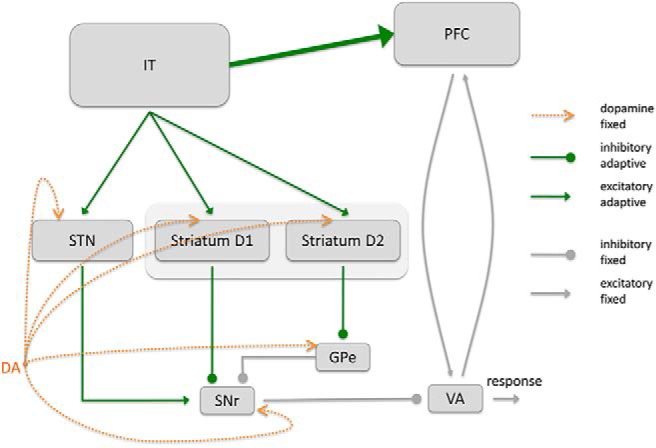
Outline of the components of the neurocomputational network to train the corticocortical, IT–PFC connection by the BG. All adaptive connections are displayed in green color. Although the IT–PFC connections are updated by Hebbian learning, the BG learn based on a three factor learning rule including a reward prediction error signal (DA). We propose that the BG bias the activity of PFC neurons that allow the PFC to learn a categorical representation.

In this rate-coding model, the membrane potential of all simulated neurons and the learning rules that determine synaptic plasticity between neighboring neurons are controlled by differential equations.

BG.

Our BG model is based on previous work (Schroll et al., 2014, 2015) and contains three BG pathways (Schroll and Hamker, 2013): the direct (striatum → substantia nigra pars reticulata), hyperdirect (subthalamic nucleus → substantia nigra pars reticulata), and short indirect (striatum → external globus pallidus → substantia nigra pars reticulata) pathways. Each of these three BG pathways obtains the input information from the IT and converges in the substantia nigra pars reticulata (SNr), a BG nucleus that tonically inhibits the ventral anterior nucleus (VA) of the thalamus.

The function of each BG pathway emerges as a learning process implemented via a three-factor learning rule that considers the presynaptic activity, the postsynaptic activity, and a dopamine (DA) signal. In our model, this DA signal estimates a reward prediction error based on the striatal activity at the time of reward delivery.

In the direct pathway, learning occurs in the projections between the IT and the striatal D1 cells and between the striatal D1 cells and the SNr. Associations between neurons in these connections become strengthened with DA bursts and weakened with DA dips as motivated by experimental data (Shen et al., 2008; Fisher et al., 2017). Therefore, this pathway learns to select a patch of VA neurons that are linked with the correct category decision, in agreement with the well known GO function of this BG pathway (Nambu et al., 2002; O'Reilly and Frank, 2006; Braak and Del Tredici, 2008; Schroll and Hamker, 2013).

In the hyperdirect pathway, learning occurs in the connections between the IT and the STN and between the STN and the SNr. Associations between neurons in these connections are also strengthened with DA peaks and weakened with DA dips (Kreiss et al., 1996; Schroll et al., 2012). Particularly, this pathway learns to suppress VA cells that encode currently unrewarded responses. Therefore, both the direct and hyperdirect pathways work together to facilitate the selection of the correct category decision, in agreement with the well known center-surround structure (Nambu et al., 2002).

In the indirect pathway, learning takes place in the projections between the IT and the striatal D2 cells and between the striatal D2 cells and GPe. In contrast to the other two BG pathways, but consistent with biological evidence (Surmeier et al., 2007; Shen et al., 2008; Fisher et al., 2017), associations between cells of this pathway become strengthened with DA dips and weakened with DA peaks. Therefore, this pathway learns to suppress VA cells linked to an incorrect category decision, in accordance with the well documented NO-GO function of this BG pathway (Apicella et al., 1992; Mink, 1996). This pathway is particularly relevant if changes in the stimulus–response associations occur.

A specific connectivity pattern is not forced on any of these plastic projections, providing our model with high flexibility. Connections are initialized in an all-to-all configuration with random low weights. The connectivity pattern is then automatically shaped through plasticity. On many previous modeling approaches of the BG, a connectivity pattern with parallel channels (one for each action or here category) was enforced without any clear account on how this arrangement could develop. Plasticity was therefore required only on early stages of the different pathways. An interesting feature of having plasticity in the late stages is that the knowledge acquired in the early stages of the pathways can be kept when learning a new task, allowing relearning to be faster than the initial learning, as shown by Schroll et al. (2012).

BG–cortex interaction.

Our model includes a cortico–thalamo–cortical pathway that allows the BG to teach category knowledge to the corticocortical pathway from IT to PFC by biasing thalamic and, thus, PFC activity. Once the category knowledge in the PFC is established, the PFC can also contribute to the final category decision by means of the cortico–thalamo–cortical pathway. Therefore, the thalamus plays a key role in integrating the category decisions produced by both the BG and the PFC.

Category information is learned in the corticocortical connections between the IT and the PFC by an unsupervised Hebbian learning rule (please refer to the discussion regarding the assumption of unsupervised learning). As the BG disinhibits the thalamus, BG will bias PFC activation, which in turn guides (DA-free) Hebbian learning in the IT–PFC connections. The PFC cells in our model slowly learn over a large number of stimuli to extract category representations, in agreement with ideas suggesting that slow learning in the cortex is required to develop category representations in the PFC (Seger and Miller, 2010). Evidence has been found for the existence of Hebbian plasticity in corticocortical long-range connections (Sjöström et al., 2001; Koch et al., 2013).

Experimental design and statistical analysis

Prototype distortion task.

In the experiment carried out by Antzoulatos and Miller (2011), two female monkeys performed a prototype distortion task in which they learned to classify stimuli into one of two different categories. We here reanalyzed data from this previous experiment as explained later.

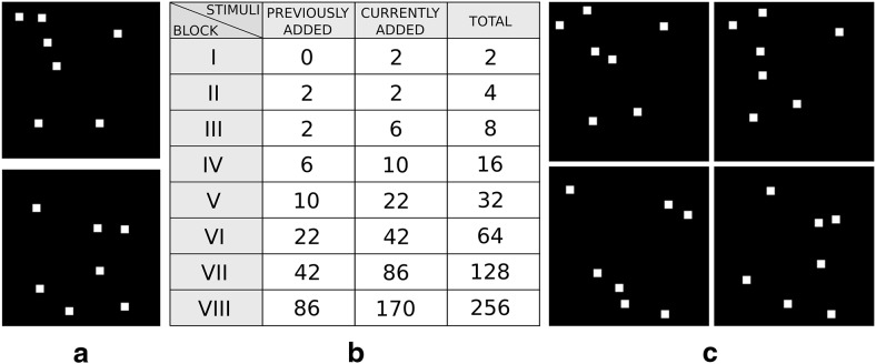
We tested our model with a very similar version of the original experiment as follows. Each stimulus was composed of 7 white small squares (7 × 7 pixels each) drawn on black background within an image of 140 × 140 pixels. Each stimulus belonged either to category A or B and was generated from the underlying category's prototype by shifting the seven squares from the prototype's coordinates randomly into nearby locations (Fig. 2a). To mimic early visual processing up to area IT, we preprocessed the images using Gaussian receptive fields (RFs) with an SD of 10 pixels (cutoff at 3.5 SDs, which equals a diameter of 35 pixels) and a sampling distance between RF centers of 15 pixels (1.5 SDs of RF size).

Figure 2.

Image examples and block description of the prototype distortion task. a, Dot prototype stimuli of two categories taken from one experimental run. b, Number and type of stimuli per block. Stimuli are distinguished according to whether they are added in the previous block or in the current block. c, Stimuli of the second block derived from the prototypes.

The set of stimuli used in each experimental run consisted of 170 stimuli per category (each generated from its category's prototype image) and was distributed into 8 blocks, where the stimulus set increased in size with each block: in each block n, the set size was 2ⁿ, equally balanced for each category. In the first block, therefore, only 2 different stimuli were presented. In the second block, 2 more stimuli were added to the set, reaching a total of 4. In subsequent blocks, only the stimuli added in the last block were kept and new stimuli were incorporated until a total of 2ⁿ was reached. Figure 2b illustrates the exact procedure. Each new block began only when 16 out of the last 20 trials were successfully performed, identical to the original experiment.

Because we aimed to focus on category learning only and did not model any eye movement or working memory components involved in the original animal task, we simplified the trial design by omitting the delay period and the oculomotor response. At the beginning of each trial, a stimulus was randomly drawn from the set of the current block and presented to the model for 550 ms. After 50 ms, we determined the model's decision using a softmax rule on a set of output neurons as follows:

where P_i is the probability of choosing category i, r_i is the rate of the output neuron associated to category i, N is the number of categories, and θ = 10⁻⁷ prevents from dividing by zero. The output neurons read our model's decision from the thalamic activity. Although 50 ms is a short time period, it is large enough for the model to reach a stable response to the presented stimulus.

In the case of a correct response, dopaminergic SNc cells were excited for 500 ms, simulating the delivery of reward (reward period). To meaningfully compare our model's results with data from monkeys, we ran a very large number of experimental runs (100,000), each with different initial synaptic weights and with slightly different values of 64 model parameters (see the mathematical model description). For each experimental run, a different set of stimuli was chosen among 100 possible sets of stimuli (each generated from two different category prototypes).

Model susceptibility to parameter variation.

To study the susceptibility of our model to modest changes in model value parameters, we computed the correlation between the model performance and each of the 64 parameters modified in the 100,000 experimental runs. Each of these correlations was computed with the Pearson correlation coefficient (PCC) using the corrcoef numpy function and considering 100,000 data pairs, each made up of the model performance and the parameter value (or the absolute value of the distance between the parameter value and the mean parameter value for a second version of the PCC) from a different experimental run. The model performance at each experimental run was evaluated by computing the average of correct trials in the last 16 trials of the experimental run.

Category selectivity.

To compare our model with the neurophysiological findings reported by Antzoulatos and Miller (2011), category selectivity was measured from model neurons' activity during the display of novel stimuli in correct trials, as previously done by the authors of the physiological experiment. As with the experimental data, category selectivity was computed within a trial-time window (size of 10 trials and 7 ms) moving in trial and time space (trial step size of 1 trial and a time step size of 3 ms). Trial time windows with less than two trials associated to one category were discarded. The d′ sensitivity index was calculated as follows:

was computed for each cell within each window, where μ_A and σ_A are the mean and SD, respectively, of the cell's firing rates recorded in trials where stimuli of category A were presented, μ_B and σ_B are the mean and SD of the firing rates recorded in trials where stimuli of category B were presented, and na and nb are the number of trials in the corresponding window that relate to stimuli of category A and B, respectively. In the striatum, we only considered cells of the direct (GO) pathway as these cells are mainly responsible for selection while cells in the indirect (NO-GO) pathway are responsible for suppression (Schroll et al., 2014).

Stimulus selectivity and category selectivity per cell.

To determine whether cells in PFC and STR become stimulus selective rather than category selective, we applied the following procedure. At the end of each block, learning was frozen and each stimulus seen so far in the experiment was presented once to the model for 50 ms, followed by a period of 100 ms without a stimulus. The response of a cell to each presented stimulus was computed by averaging the cell's activity over 50 ms presentation time and normalized by its maximum response to all stimuli within a block.

We defined a stimulus selectivity index (SI_stim), which measures whether a cell is particularly tuned to a single stimulus compared with the rest of the stimuli belonging to the same category as follows:

where s is a presented stimulus, S is the set of presented stimuli, R_s is the cell's response to s, and R̄_s is the mean cell's response to those stimuli in S that are different from s and belong to the same category as s.

Category selectivity (SI_cat) was measured by computing the absolute value of the difference between the cell's mean response to stimuli of one category and the cell's mean response to stimuli of the other category (i.e., the numerator of the d′ sensitivity index) as follows:.

where R̄_A is the mean cell's response to the stimuli that belong to category A and R̄_B is the mean cell's response to the stimuli that belong to category B.

We did not compute the full d′ sensitivity index because we wanted the stimulus selectivity and the category selectivity to be plotted in the same scale. Therefore, the category selectivity was normalized in the same way as the stimulus selectivity (via normalizing the responses of each cell).

Only experiments that learned to criterion (in each block 16 out of 20 consecutive trials have to be correctly classified before the maximum number of trials determined in each block is reached) were considered for the analysis.

Face categorization task.

To test the model's performance in a real-world classification scenario, we created an additional face categorization task. Face pictures of George W. Bush and Bill Clinton were extracted from videos and presented to the model for classification purposes.

All videos were taken from the YouTube Faces Database (Wolf et al., 2011), which consists of 3425 videos of 1595 different people, downloaded from YouTube and manually annotated. The shortest clip duration was 48 frames, the longest clip consisted of 6070 frames, and the average length of a video clip was 181.3 frames. For Bill Clinton, we obtained four videos with a total of 851 frames and, for George W. Bush, we obtained five videos with a total of 820 frames.

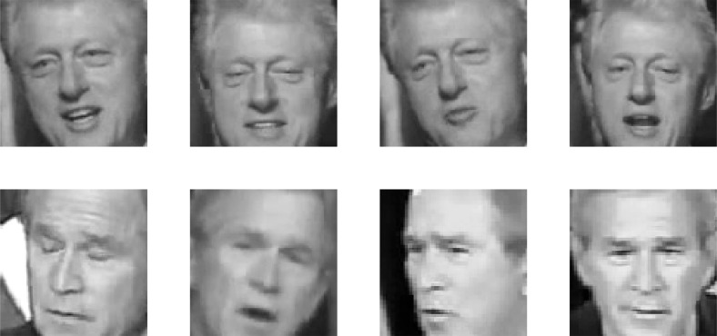
For each frame, the face region was detected using a Viola–Jones filter (Viola and Jones, 2004), allowing us to extract and resize each face to a 100 × 100 grayscale image. Figure 3 shows a few examples of the resulting face images.

Figure 3.

Examples of face stimuli presented to the model. The upper row of pictures correspond to the category of Bill Clinton, the lower row of pictures to the category of George W. Busch. Each picture shows a face with a particular expression and from a different perspective. Each greyscale image has a size of 100 × 100 pixels and was obtained by applying a Viola–Jones filter to a particular frame of a YouTube video.

To obtain high-level facial features that mimic the computation in visual areas, we trained a neural network using the keras library (https://keras.io/) and the Theano backend (http://deeplearning.net/software/theano/). The training set consisted of all the images obtained from the YouTube Faces Database except those of George W. Bush and Bill Clinton, providing us with 619,455 input images of 1593 people (labels).

The neural network starts with a single convolutional layer, extracting 16 filters of size 6 × 6 and using a rectified linear transfer function (ReLU). It is followed by a max-pooling layer over 2 × 2 units and a dropout layer with p = 0.5. This layer feeds a fully connected layer (100 neurons, ReLU transfer function and dropout 0.5), which itself feeds a softmax layer with 1593 neurons (one per label).

The network was trained by minimizing the categorical cross-entropy between the true labels and the predictions using the stochastic gradient descent method, with minibatches of 100 samples, an initial learning rate of 0.01 decaying by 10⁻⁶ in each epoch, and a Nesterov momentum of 0.9. After 100 epochs, the network obtained an accuracy of 99.2% on a test set composed of 61,945 randomly selected samples (10% of the whole data, not used for training). Finally, the high-level facial features for category learning of Bush and Clinton images were extracted by taking the neural activation before the last softmax layer.

Mathematical model description.

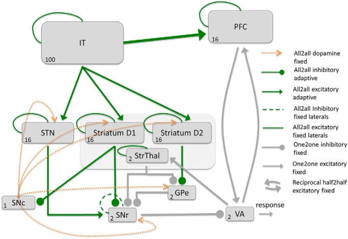
The neurocomputational model was implemented using the ANNarchy neural simulator (Vitay et al., 2015) version 3.0. The forward Euler method had been used to numerically solve these differential equations with a time step of 1 ms. Figure 4 shows our model' architecture with more detail than in Figure 1 by illustrating the number of cells in each neural population, all of the connections in the model, and the type of these connections.

Figure 4.

Detailed outline of the components of the neurocomputational network. The number of cells that each neural population has is shown at the bottom left corner of each population box. The reward prediction error signal used by the BG to learn is generated at SNc. StrThal, Striatum with thalamic afferents.

IT.

IT is composed of 100 neurons with membrane potentials that are computed by the following:

where m_j^IT is the membrane potential of the neuron j, τ_m = 10 ms is the time constant, and S_j is the part of the preprocessed image that this neuron receives. The firing rate r_j^IT(t) is calculated by applying ( )⁺ to the membrane potential, where ( )⁺ is a function that takes the positive part of its argument (all negative arguments are transformed to 0)

BG.

The BG model is based on the one by Schroll et al. (2014). We again briefly describe the model and highlight the changes that we implemented.

The membrane potential of all cells in the BG is defined by a leaky integration equation as follows:

where m_j is the membrane potential of neuron j, τ_m = 10 ms is the time constant, B_j is the baseline of the cell's membrane potential (2.4 for the SNr, 1.0 for the GPe and 0.4 for the other nuclei), ϵ_j(t) is random noise sampled from a uniform distribution in the interval [−1.0, 1.0] for the GPe and SNr, and [−0.1, 0.1] for the other nuclei; I^pre is the input from the presynaptic neural population to neuron j, N_y is the set of presynaptic neural populations with inhibitory synapses to neuron j, and N_e is the set of presynaptic neural populations with excitatory synapses to neuron j.

The inputs are computed as follows:

where w_i,j(t) is the weight of the synapse between the presynaptic neuron i and the postsynaptic neuron j, and r_i^Pre(t) is the firing rate of the presynaptic cell i.

Equation 7 is used to compute the impact of all the connections in our model except for the case of the SNr lateral connections. The model includes plasticity in connections from the striatum and the STN to the SNr. Although uncommon, this approach gives the model a high level of flexibility because it does not force a particular connectivity pattern, but rather lets the network develop it by itself. Unfortunately, except for the striatum, little is known about neural plasticity in the BG. As reviewed by Schroll and Hamker (2013), not only the striatum, but other nuclei are innervated by axons of DA neurons. Further, administration of the DA precursor levodopa has been shown to affect synaptic plasticity in SNr (Prescott et al., 2009). DA-dependent plasticity in our model SNr prevents striatal cells from being hard wired to a single category, as would be the case in previous models of BG which lack this plasticity. Further, learning requires competition between cells, otherwise all neurons would learn similar features. To implement competition in the SNr, the impact of the SNr lateral connections is computed by multiplying the synaptic weights by a reversal factor (1 − r_i^Pre(t))⁺ as follows:

where the synaptic weights of the lateral connections in the SNr are excitatory and fixed to 1. There is no direct evidence for our assumed SNr circuitry, mainly due to a lack of studies, but our assumption agrees with data showing that activations of the direct pathway cells in the striatum can elicit both excitation and inhibition of SNr neurons (Hikosaka et al., 1993; Freeze et al., 2013). Lateral connections in the striatum D1 (StrD1), striatum D2 (StrD2), and STN are inhibitory and set to 0.3.

SNc follows an equation that produces the DA signal and is the only part of our network that is not governed by Equation 6 as follows:

where B_DA = 0.1 is the baseline of the cell's membrane potential, I_j^StrD1(t) is the impact from the connections of all StrD1 cells to the SNc that learn to represent the reward prediction at the time of the reward delivery, and R is a term that changes depending on whether reward is delivered (set to 1) or omitted (set to 0). The DA signal is only computed during the reward presentation period and it encodes a reward prediction error at the time of the reward delivery using D1 striatal neurons activity for the prediction because these cells have been reported to be part of the pathway that project to the dopaminergic neurons (see Vitay and Hamker, 2014 for a more detailed model of the reward prediction error computation).

The firing rate of all cells in our model is calculated by applying ( )⁺ to the membrane potential. The learning rule to update the synaptic weights from the IT cells to the 16 StrD1 cells, 16 StrD2 cells, and 16 STN cells is as follows:

with C being the covariance term as follows:

f_DA(x) is a function that determines how DA influences learning (where T_d = 1 for cells in the direct and hyperdirect pathway and T_d = −1 for cells in the indirect pathway) as follows:

and α_j the adaptive normalization variable (T_c = 1 for excitatory connections and T_c = −1 for inhibitory connections) as follows:

Where τ_w = 75 ms is the time constant. Synapses are randomly initialized with a uniform distribution in the interval [0.0, 0.3].

With DA peaks, very active StrD1 and STN cells will strengthen their connections with the active IT cells and weaken their connections with the rest of IT cells. With DA dips, the connections between very active StrD1 and STN cells and active IT cells weaken. The DA learning effect is reversed in the projections from IT to StrD2 cells. Therefore, with DA dips, the most active StrD2 cells will strengthen their connections with the active IT cells and weaken their connections with the rest of IT cells. With DA peaks, the connections between very active StrD2 cells and active IT cells weaken.

The covariance term C depends on the following parameters and variables: the firing rate of the postsynaptic cell r_j^POST(t), the mean of the firing rates in the postsynaptic layer r̄^POST(t), a threshold γ_pre = 0.15, the firing rate of the IT neuron r_i^IT(t); and the mean firing rate in the IT layer r̄^IT(t). f_DA(x) depends on the DA level DA(t) and the DA baseline B_DA = 0.1.

The subtractive term of the right side of Equation 10 serves to saturate the synaptic weights of a cell so that the cell's firing rate is also bound. Equation 13 shows that α_j^POST depends on the membrane potential of the postsynaptic cell, m_j(t), and a threshold, m^MAX = 1.

The learning rule for changing the connection from the StrD1 to the SNr, from StrD2 to GPe cells, and from STN to SNr cells is as follows:

with the covariance term as follows:

where f_DA(x) is the variable that determines how DA influences learning via Equation 12, α_j is the adaptive normalization variable computed via Equation 13, and τ_w = 50 ms is the time constant. Synapses are randomly initialized by values taken from a uniform distribution in the interval [0.0, 0.05].

The additive term on the left side of Equation 14 ensures that, during peaks of DA, the most active StrD1 cells will strengthen their connections with the less active SNr cell and weaken their connections with the other SNr cell and the most active STN cells will strengthen their connections with the most active SNr cell and weaken their connections with the other SNr cell. With DA dips, the most active StrD1 cells will weaken their connections with the less active SNr cell and the most active STN cells will strengthen their connections with the less active SNr cell.

In the case of the StrD2–GPe projections, the DA learning effect is the opposite of the DA effect in the StrD1–SNr projections. With DA dips, the most active StrD2 cells will strengthen their connections with the less active GPe cell and weaken their connections with the other GPe cell. With DA peaks, most active StrD2 cells will weaken their connections with the less active GPe cell.

C depends on the following parameters and variables: a threshold γ_post = 0.15, the firing rate of the presynaptic neuron r_j^PRE(t), the mean of the firing rates in the presynaptic layer r̄^PRE(t), the firing rate of the postsynaptic cell r_j^POST(t), and the mean of the firing rates in the postsynaptic layer r̄^POST(t).

The threshold of α_j^POST is m^MAX = 1 for the StrD1-SNr connections, m^MAX = 2.6 for the STN-SNr connections, and m^MAX = 2 for the StrD2-GPe connections. The SNr and GPe also receive thalamic feedback which is provided by direct connections from the VA to a subpopulation of striatal cells (StrThal in Fig. 4), that in turn project to both the GPe and the SNr. These projections help to stabilize the BG decision by enhancing the inhibition of the selected category in the SNr. This stabilization allows to reliably notify the BG pathways which category decision should be reinforced when a DA peak is generated (Brown et al., 2004). The connections from the StrThal to the SNr and GPe are set to 0.3, from the VA to the StrThal to 1, and the lateral connections in StrThal to 0.3.

The connections from the StrD1 cells to the SNc cell are updated by Equations 16 and 17 as follows:

with

where τ_w = 100,000 ms is the time constant, r_j^StrD1(t) is the firing rate of the neuron j in the StrD1 layer, r̄^StrD1(t) is the mean of the firing rates in the StrD1 layer, g_DA is a parameter that scales the effect of DA dips and peaks in learning; DA(t) is the DA level, and B_DA is the baseline of the DA level. Therefore, peaks in DA will strengthen the connections between the SNc cell and the most active StrD1 cells and dips will weaken these connections.

Finally, we summarize the difference between our model and the one by Schroll et al. (2014). Because our examples required only two categories to learn, our SNr and GPe are composed of two cells instead of four. As a result, the synaptic values of the SNr lateral connections are fixed to 1.0 instead of being plastic. The synaptic values of the plastic connections in the model are randomly initialized from a uniform distribution; instead, Schroll et al. (2014) initialized these synaptic weights to zero. The projections from the IT to the BG input nuclei are only excitatory in our model. In contrast, Schroll et al. (2014) allowed these synaptic weights to switch their character between excitatory and inhibitory during learning. Learning in the present model does not rely on calcium traces implemented in the previous model because they are not required for the purposes of this study. The learning rules from the IT to the BG input nuclei have been slightly changed (in the subtractive term of the learning rules). Finally, the time constant of the IT membrane potential, the m^MAX for the STN–SNr connections and the fixed weights of w^SNr-VA were modified.

Cortico-thalamic architecture.

The membrane potential m_j of the 2 VA and the 16 PFC cells is computed by the Equations 6 and 7 with a time constant of 10 ms, the random noise is generated from a uniform distribution in the interval [−0.05, 0.05] for the PFC and in [−0.0001, 0.0001] for the VA, and the baseline is 0 for both populations. The firing rate is calculated by applying ( )⁺ to the membrane potential.

The connectivity between PFC and VA is fixed and ensures that a PFC cell can only obtain its input from a single VA cell to avoid any overlap. The number of PFC cells connected to a VA cell is balanced equally. The weight values are defined as follows: w^VA-PFC, w^PFC-VA, and w^PFC-PFC are fixed with values 0.35, 0.15, and 0.1 respectively. w^IT-PFC are randomly initialized with a uniform distribution in the interval [0.2, 0.4] and modified by the following learning rule:

where τ_w = 15,000 ms; γ_pre = 0.15, and α_j^PFC(t) is the variable that contributes to the dynamic synaptic saturation (Eq. 13), with threshold m^MAX = 3.5.

In the most active PFC cells, the synapse will be strengthened if the presynaptic cell's firing rate is above the population mean and will be weakened otherwise. The subtractive term on the right side of Equation 18 ensures dynamic synaptic saturation as in the Oja's learning rule (Oja, 1982).

Variation of 64 model parameters.

Each of the 100,000 simulations was performed with different values for 64 model parameters. The value of each of these parameters was randomly selected from a uniform distribution in the interval between ±10% of the parameter's value previously specified in the mathematical model description. The 64 model parameters are as follows: the membrane potential's baseline for the different neural populations, the membrane potential's noise for the different populations, the time constant of the different learning rules, the m^MAX of each learning rule, the γ_pre of each learning rule, the scaling factor for DA peaks and the scaling factor for DA dips in the f_DA(x) of each projection, the scaling factor for the reward prediction signal when reward is not delivered, the value of g_DA when reward is not delivered, and the synaptic weights of the different fixed connections.

Results

Simulation results

To meaningfully compare our model's results with physiological and biological data and, at the same time, test the robustness of our model, we ran 100,000 category learning experiments, each with randomly generated initial synaptic weights and with randomly generated values for 64 model parameters. Each of these parameters' values was randomly determined from a uniform distribution in an interval between plus/minus 10% of its value specified in the Materials and Methods section (base value). With a total of 100,000 of these experimental runs, we consider a large number of variations for the 64 model value parameters. Further, we used some variability in the learning task by choosing for each experimental run a different set of stimuli among 100 possible sets of stimuli, each generated from two different category prototypes.

An experiment was considered successful when, within 65 trials per block, 16 out of 20 consecutive trials were correct in each block. The model successfully executes 82,639 out of 100,000 experiments (82.639%), a proportion slightly better than that of monkeys (Antzoulatos and Miller, 2011): 19 of 24 (79.166%). Further, the model shows a similar learning performance across the paradigm than that of monkeys (Fig. 5): initially, the model randomly selects a category (50% correct performance); the performance gradually improves from the first block to the fourth block; and, from the fifth block on, the performance saturates at ∼96.5%.

Figure 5.

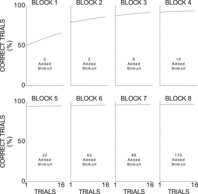
Model performance across blocks for categorizing novel stimuli averaged from 82,639 experiments. Because each block had a minimum of 16 trials (due to the criterion to succeed in a block), we analyzed only the first 16 trials per block. Applying a sliding three-trial window, we then measured the percentage of correct trials for each relevant trial across the all successful experiments (black line) and the corresponding SEM. The obtained SEMs are too small to be shown in this plot (smaller than 0.002) due to the large number of experiments considered in this analysis.

The PCC between each of the 64 parameters and the model's performance (computed for each experimental run as the percentage of correct trials in the 16 last trials) is very low: between −0.035 and 0.041, indicating that the model tolerates modest changes in any of the specified model value parameters. When the PCC considered the absolute values of the perturbations produced in each parameter base value instead of the values of each parameter, correlations are even smaller: between −0.01 and 0.01.

Importantly, our model reproduces the key neurophysiological findings of Antzoulatos and Miller (2011): at the beginning of the paradigm, striatal cells are strongly category selective and PFC cells are weakly category selective, whereas PFC cells later become highly category selective and striatal cells weakly category selective (Fig. 6).

Figure 6.

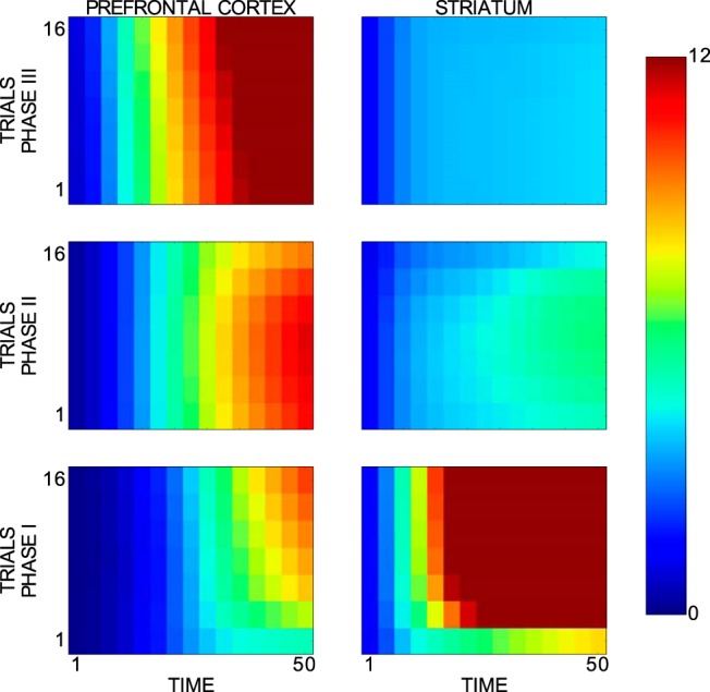
Mean d′ sensitivity index for category selectivity of neurons in the model's PFC and striatum. Horizontal and vertical axes refer to time and trials, respectively. The first phase represents the first two blocks, the second phase the next two blocks, and the last phase the last four blocks. Only successful experiments (82,639 experiments) and successful trials of novel stimuli were considered in this analysis. The analyzed data spread across a time interval spanning from cue onset to reward onset. Each phase includes only its first 16 trials (i.e., seven trial windows). Different values for the 64 model parameters were set at the beginning of each experimental run.

In the following, we used the model as a tool to better understand this key finding. When analyzing each cell's category and stimulus selectivity over 100 simulations (with fixed model parameters), we see that PFC and striatal cells show a different selectivity profile (Fig. 7). Throughout the paradigm, there are striatal cells that are stimulus selective and striatal cells that are category selective, indicating that striatal cells encode both specific and abstract knowledge. Importantly, this result shows that, although the striatum d′ sensitivity is reduced late in the experiment, there are striatal cells involved in category learning throughout the whole experiment. PFC cells, in contrast, increase their category selectivity across blocks whereas their stimulus selectivity remains low throughout the paradigm, supporting that these cells encode generalized, categorical knowledge.

Figure 7.

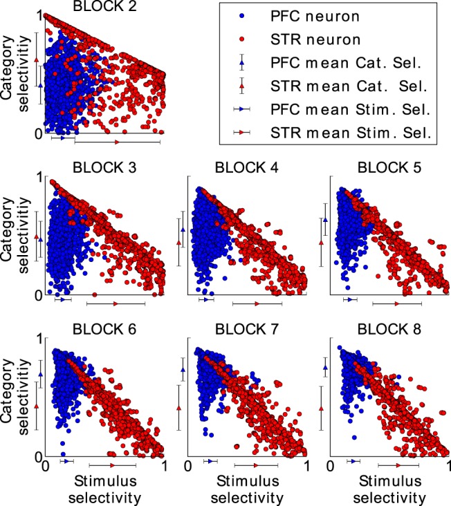
Category and stimulus selectivity for each model cell in the striatum (red dots) and in the PFC (blue dots) in all successful experiments. Both selectivities were measured at the end of each block as outlined in the Materials and Methods section. The first block was omitted because there was only one stimulus per category, so stimulus selectivity could not be computed. A maximum category selectivity of 1 indicates that the corresponding cell responds maximally to all stimuli of one category and becomes inactive for the stimuli from the other category. Maximum stimulus selectivity, in contrast, indicates that the corresponding cell responds to a single stimulus with maximum activity, but that it remains inactive for the rest of the stimuli from the same category. Although the category selectivity in the PFC clearly increases with each block,the category selectivity in the striatum does not and cells stay stimulus selective. The mean category and the mean stimulus selectivity of the PFC and STR cells is shown at each axis by a blue and red triangle, respectively. Error bars indicate the SD.

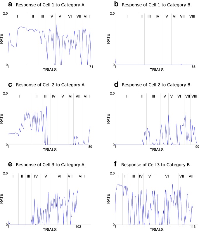
Three example striatal cells illustrate different response characteristics to stimuli of both categories (Fig. 8). The first cell exclusively responds to stimuli of one category throughout the experiment, but from block IV onwards, it does not respond to all stimuli of its preferred category. Therefore, its category responses become more variable within the set of stimuli of the preferred category. The second cell switches its category selectivity. Furthermore, the variability of this cell's category response is higher in the last blocks than in the first blocks. A third cell responds to stimuli of one category in the first blocks, but becomes selective to stimuli of the other category in the later blocks as well. Therefore, this cell loses its category selectivity and appears to become selective to input patterns common to both categories.

Figure 8.

Firing rates of three typical striatal cells plotted across all trials of one experimental run subdivided for presentation of stimuli from category A (left subplots) and category B (right subplots). The seven vertical lines indicate borders between the eight blocks (I, II, III, IV, V, VII, and VIII). a, firing rate of cell 1 across the trials that present a stimuli of category A in one experimental run. b, firing rate of cell 1 across the trials that present a stimuli of category B in the same experimental run. c and d show the same as a and b but for cell 2. e and f show the same as a and b but for cell 3. The 64 model parameters were set to their base values.

When we analyze the response characteristics across all cells, we observe that the distance between the mean response to the preferred category μ_P and the mean response to the nonpreferred category μ_N reduces after the first phase due to a reduction in μ_P and a small increase in μ_N (Fig. 9a). However, the mean response to the preferred category stays much higher than the one to the nonpreferred category in all three different phases of the experiment, showing that striatal cells have on average a clearly preferred category throughout the experiment. Therefore, a cell responding to both categories (Fig. 8) is not the typical case.

Figure 9.

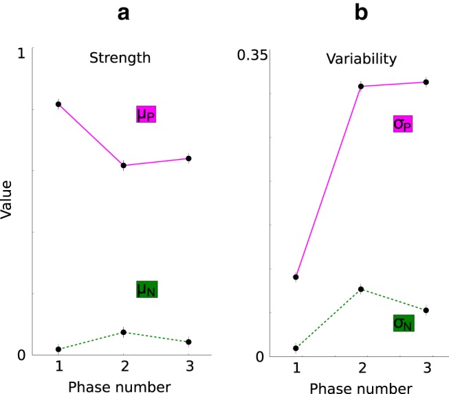
Model prediction with respect to the individual components of the d′ sensitivity index of the striatum. The values are computed at the last trial time bin of each phase and from the same simulation recordings used to obtain the STR d′ sensitivity index in Figure 6. a, Mean response to the preferred category (dots in magenta line, μ_P) and to the nonpreferred category (dots in green line, μ_N) per phase. The preferred category is the category for which each STR cell responds on average most strongly in each single trial time window. b, Mean SD of the response to the preferred category (dots in magenta line, σ_P) and to the nonpreferred category (dots in green line, σ_N) per phase.

The increase in the SD of the response to the preferred category σ_P and the SD of the response to the nonpreferred category σ_N (Fig. 9b) confirms our observations of the example cells in that the striatal response to category information becomes more variable after the first phase of the experiment.

Because these results suggest that the decrease in μ_P − μ_N is due to an increase in the variability of the category response, our model predicts that the decrease of the d′ sensitivity index is primarily the result of an increase in the variability of the category response.

We next explored why the decrease in striatal category selectivity and the accompanying increase in variability occurred. As a first hypothesis, we reasoned that, as PFC category selectivity increases with learning, striatal category selectivity becomes less required for successful task performance and is therefore unlearned because the neural activity in the striatum may not be the cause of the final decision. To test this hypothesis, we ran 100 additional simulations with our model, but we now blocked learning in the PFC so that the BG were performing the experiment alone. However, the striatal d′ sensitivity index abruptly decreases after the first phase and stays at a low level in the next two phases, qualitatively very similar to the full model, thus ruling out that the decrease in striatal category selectivity occurs due to a PFC dominance in later blocks.

As another hypothesis, we tested whether, as task performance increases, DA peaks (i.e., positive reward prediction errors) in the model stop appearing, which would impair further learning in the striatum. However, DA peaks are only reduced to 43% on average, enough to still produce large synaptic changes in the striatum.

Next, we tested whether the increase of the variability in the striatal category response and therefore the decrease of the striatal category selectivity is produced by the learning of a large diversity of stimuli. To test this idea, we ran 100 simulations with the full model performing a new prototype distortion task in which the diversity of exposed stimuli is large and constant from the beginning of the task. Rather than subdividing the prototype distortion task into blocks with increasing numbers of stimuli across blocks, any stimulus from the whole repertoire of stimuli available per experiment could be presented in each trial. We now observed a low striatal category selectivity from the beginning of the experiment (Fig. 10) and no drop in the selectivity index. Because PFC category selectivity rises to high values, the BG still teach PFC cells to develop category representations, indicating that the BG are involved in the categorization task. Therefore, this result supports that the decrease in the d′ sensitivity index is due to the fast learning of a large diversity of exposed stimuli, which makes it impossible for the striatal cells to acquire complete category representations and to respond to all stimuli of the preferred category. Therefore, the fact that the d′ sensitivity index in this revised experiment is low from the beginning discards a PFC dominance in the category decision and an omission of DA peaks as reasons for the low striatal category selectivity because both effects occur later in the experiment.

Figure 10.

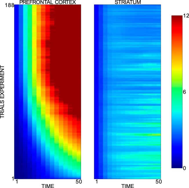
Averaged d′ sensitivity index across trials and time for the PFC and the striatal activities recorded in a prototype distortion task without blocks. Horizontal and vertical axes refer to trials and time, respectively. The subplots on the left and right side belong to PFC and striatal recordings, respectively. Only successful experiments and successful trials of novel stimuli were considered in this analysis. The analyzed data spread across a time interval spanning from cue onset to reward onset. The 64 model parameters were set to their base values in all considered simulations.

To further explore BG and PFC interactions, we compared the performance of the full model with the performance of the BG and the PFC alone in a slightly more challenging, real-world category learning task. In each of the 2500 trials of this task, an image randomly selected from 1671 images of Bill Clinton and George W. Bush (extracted from YouTube videos and therefore varying in perspective and facial expressions) was presented to the model for classification purposes. To mimic early visual perception up to area IT, we used a convolutional network trained on other faces to transform each image into a 100-dimensional vector representing the high-level facial features of the corresponding image (see Materials and Methods). To adapt the model to these new inputs, two small changes were implemented. First, slower learning in the PFC (τ_w = 100,000 ms) was required to guarantee that the common patterns among inputs of a category were extracted. Second, the presynaptic threshold in the PFC learning rule was set to γ_pre = 0.0 to ensure that all relevant features of the input space were learned. Surprisingly, the BG model alone achieves a much weaker performance than the full model and the PFC alone (Fig. 11). The BG and the full model very soon reach 85%. Whereas the full model slowly improves its performance, finally achieving a level of 97.4%, the BG alone lack further improvement and their performance fluctuates at ∼85%. The performance of the PFC alone, with 95.6% of correct responses after the training of the full model, is only 1.8% lower than the full model's performance. Therefore, with a difference in performance between the full model and the BG alone of ∼12.2% and a difference in performance between the PFC alone and the BG alone of ∼10.4%, we can corroborate the relevant role of the PFC in pushing the categorization performance to high levels with complex input stimuli. We have also found that Hebbian learning alone is not enough to reach a high performance on the task.

Figure 11.

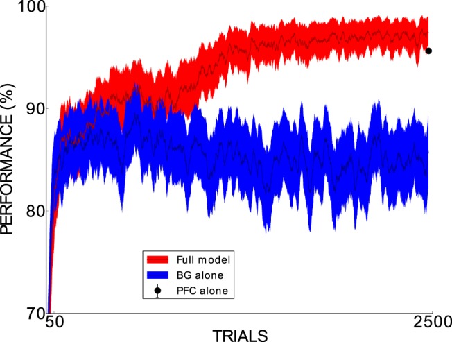
Across-trial performance of the full model (dark red line) and the BG-alone model (dark blue line) across the 2500 trials of the task with real-world face stimuli. For each of the 2500 trials, performance was averaged across 100 experimental runs. Moreover, SEMs were computed (filling color around the lines). A 25-trial window was used to smooth the plot. The black dot in the final trial represents the mean performance of the PFC alone in an extra set of 1000 trials performed at the end of the 2500 trials across 100 experimental runs. The corresponding SEM is 0.00065, too small for being shown in the plot as the dot's error bar. The 64 model parameters were set to their base values in all considered simulations.

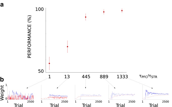
To ensure that the slow learning in the PFC is key for pushing the categorization performance of the full model above the BG categorization performance, we compared the categorization performance of five full model configurations each with different learning speed in the PFC. Categorization performance was here evaluated across 100 runs on the category learning task of faces. Figure 12a illustrates that the full model's performance increases as the speed in the PFC learning rule decreases, confirming the principal role of the slow learning in the PFC for achieving high categorization performance.

Figure 12.

Effect of different PFC learning speeds on the full model's performance in the learning task with real-world faces images. a, τ_STR is the time constant of the learning rule in the striatum and was equal to 75 ms. τ_PFC is the time constant of the learning rule in the PFC and its different values here studied were 75, 975, 33375, 66675, and 100000 ms. Each red dot shows the mean performance across 100 experimental runs at the last trial (trial 2500). Error bars indicate the corresponding SEMs. b, Example (for each different condition) of PFC weight trajectory (red line) and STR weight trajectory (blue line) across the trials of one experimental run. The weight value was normalized via dividing by the maximum weight value of the recorded PFC and STR cells. In all considered simulations, the 64 model parameters were set to their base values except for the learning rule time constant in the PFC, which was set to the value specified by each condition.

To determine whether slow learning alone can be sufficient, we ran the BG alone with slow learning in an additional region of the striatum. However, the BG with slow learning reach a significantly lower performance (∼17.4% lower) than the full model (Fig. 13). Also, to study the effect of additional basal–ganglio–cortical connections seen in vivo, we added to our model the well known connection from the PFC to the STR (Ferry et al., 2000). Figure 13 shows that this version of the model does not alter the performance previously achieved by our full model, indicating that this connection does not have a relevant effect on the simulated task.

Figure 13.

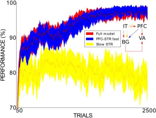
Across-trial performance of the full model (dark red line), the full model with an extra connection from the PFC to the STR (dark blue line), and a model with the slow learning in the STR instead of the PFC (gold line) across the 2500 trials of the task with real-world face stimuli. For each of the 2500 trials, performance was averaged across 100 experimental runs. SEMs are also shown (filling color around the lines). A 25-trial window was used to smooth the plot. The 64 model parameters were set to their base values in all considered simulations. The small model sketch summarizes the main difference between the three models.

Physiological results

Even though the striatum d′ sensitivity index abruptly decreases after the first phase, our model predicts that on average, the striatal cells remain selective for a preferred category, but their response to category information becomes more variable (Fig. 9). To test these predictions empirically, we went back to the original monkey data. In accordance with our simulation results, the monkey data shows that the mean response to the preferred category μ_P weakly decreases after the first phase and that the mean response to the nonpreferred category μ_N slightly increases after the first phase (Fig. 14a). Most importantly, μ_P is significantly higher than μ_N in the three phases, confirming that, although the striatum d′ sensitivity index shows a large decrease, the striatal cells show a preferred categorical response in the course of the experiment.

Figure 14.

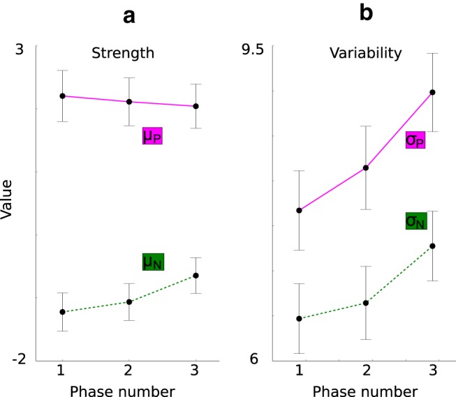
Analysis of the individual components of the striatum d′ sensitivity index computed from the monkeys' recordings obtained in the cue period. For each phase, the last trial time bin is plotted. a, Mean response to the preferred category (dots in magenta line, μ_P) and to the nonpreferred category (dots in green line, μ_N) per phase. The preferred category is the category for which each STR cell responds on average most strongly in each single trial time window. Because neural spiking activity tended to rise with time of recording, we had to correct the neural firing rate to the pretrial baseline and thus the negative average firing rate for the nonpreferred category. b, Mean SD of the response to the preferred category (dots in magenta line, σ_P) and to the nonpreferred category (dots in green line, σ_N) per phase.

In agreement with our model, the monkey data show that both the variability of the striatal response to the preferred category σ_P and the variability of the striatal response to the nonpreferred category σ_N increases after the first phase, while σ_P is higher than σ_N (Fig. 14b).

Discussion

We introduced a new neurocomputational model of category learning to investigate interactions of BG and PFC. Although it is known that the PFC receives a dopaminergic input, although less than the striatum (Seger and Miller, 2010), its phasic properties are less pronounced due to the very slow decay of DA in PFC as reviewed by Lapish et al. (2007). Lapish et al. (2007) suggested that the corelease of glutamate from DA neurons may serve as a temporally precise signal to allow PFC neurons to switch between different modes that affect local network dynamics. However, how such DA-dependent states may subserve reinforcement learning of corticocortical connections has not been discussed. Therefore, we take the conservative assumption that corticocortical connections follow a Hebbian learning rule. However, Hebbian learning is insufficient for categorizing complex input stimuli at high performance levels. Therefore, the PFC requires teaching signals to guide learning toward useful representations at an intermediate level between perception and action. We here explored the hypothesis that the BG modulate the cortico–thalamo–cortical loop and thus provide the PFC with the required task related information. Unlike the mesocortical DAergic signal, the BG teaching signal provides no reward related information to the PFC. It supplies the PFC with a desired response for the current input as estimated by the BG. Interestingly, the “teacher” can display a much lower performance than the “student” (Fig. 11). Due to the slow learning of the corticocortical connections (here, IT–PFC), occasionally wrong decisions transferred by the BG are tolerated. The BG with 85% correct performance will still teach the PFC to push the model's performance up to almost 100%. Potential benefits of combined fast and slow learners have been laid out in the context of memory consolidation based on models of the cortex and hippocampus (McClelland et al., 1995; O'Reilly and Rudy, 2000), but although the main ideas are intuitive, clear model demonstrations have been rare since then. Our simulation results underline these previous ideas, here with respect to BG–PFC interactions, and clearly demonstrate the additional advantage of a slow learning system that complements fast learners, which is required for survival.

As our model replicates key behavioral and physiological data of macaque monkeys performing a prototype distortion task (Antzoulatos and Miller, 2011), our model provides some confidence to allow us to further delineate the potential mechanistic causes behind the observation that striatal neural activity is initially a good predictor of stimulus category, whereas this category selectivity declines as the number of stimuli to classify increases. Our simulations suggest that the drop in striatal category selectivity does not relate to a disengagement of the striatum in category learning: the striatal cells' response to category information exhibits, on average, a strong preference to one category throughout the whole experiment, indicating that striatal cells can acquire category knowledge when learning to classify a large number of stimuli. Importantly, our model predicts that the decrease in the category selectivity of striatal cells occurs due to an increase in the variability of the category response. We tested and confirmed this model prediction by reanalyzing the original monkey data obtained by Antzoulatos and Miller (2011). The large number of simulations (100,000), each performed with different model value parameters, ensures that the results are robust to modest changes in these parameters. The model does not show significant susceptibility to changes in any of these parameters.

Our results may advance the field of computational models of category learning, which already has a long tradition. Category learning models with a more psychological focus typically tend to abstract from details of brain computation and focus mainly on a replication of behavioral data in different category learning tasks such as prototype, probabilistic, rule-based, and information–integration categorization tasks (for review, see Richler and Palmeri, 2014). Most recent neurocomputational models of category learning focus on the role of the ventral visual pathway, but typically simplify at the level of category decision by relying on mechanisms of supervised learning to link feature and object information to categories (Serre, 2016). However, Cantwell et al. (2017) also emphasized the role of the BG in category learning by merging a model of visual object processing with a model of procedural learning based on the direct pathway of the BG. Although this is interesting, their model has been directed to learn correct stimulus–response associations and to match the performance of human behavioral data in category learning; it did not focus on the formation of category representations in PFC and likewise has not been used to explain electrophysiological data such as those from the study of Antzoulatos and Miller (2011). Our model demonstrates that the PFC can be trained by the BG to develop useful internal representations for completing a prototype distortion and a simple, but real-world face categorization task. Because this learning is generic, it may also provide the basis of other category learning tasks, although some of them may recruit additional or slightly different brain areas (Seger and Miller, 2010; Richler and Palmeri, 2014) and may therefore require more complex models.

Because the BG form multiple loops with most parts of cortex (Alexander et al., 1986; Haber, 2003), our model could provide an inspiration for the organization of other loops as well. A further challenging and unanswered question is how different cortical areas connect with each other across loops. The organization of connections in early sensory areas may be approximately well explained by Hebbian learning. Corticocortical areas further downstream likely require error signals and fast learning BG circuits to bias cortex in a meaningful way so that brain circuits self-organize to find solutions that allow the organism to survive, reproduce, and evolve. Hélie et al. (2015) already suggested that the BG are required for learning such corticocortical associations. Our study provides an example of how this may actually work and may offer a blueprint for the organization of other corticocortical associations.

References

- Alexander GE, DeLong MR, Strick PL (1986) Parallel organization of functionally segregated circuits linking basal ganglia and cortex. Annu Rev Neurosci 9:357–381. 10.1146/annurev.ne.09.030186.002041 [DOI] [PubMed] [Google Scholar]
- Antzoulatos EG, Miller EK (2011) Differences between neural activity in prefrontal cortex and striatum during learning of novel abstract categories. Neuron 71:243–249. 10.1016/j.neuron.2011.05.040 [DOI] [PMC free article] [PubMed] [Google Scholar]
- Antzoulatos EG, Miller EK (2016) Synchronous beta rhythms of frontoparietal networks support only behaviorally relevant representations. eLife 5:e17822. 10.7554/eLife.17822 [DOI] [PMC free article] [PubMed] [Google Scholar]
- Apicella P, Scarnati E, Ljungberg T, Schultz W (1992) Neuronal activity in monkey striatum related to the expectation of predictable environmental events. J Neurophysiol 68:945–960. 10.1152/jn.1992.68.3.945 [DOI] [PubMed] [Google Scholar]
- Braak H, Del Tredici K (2008) Cortico-basal ganglia-cortical circuitry in parkinson's disease reconsidered. Exp Neurol 212:226–229. 10.1016/j.expneurol.2008.04.001 [DOI] [PubMed] [Google Scholar]
- Brown JW, Bullock D, Grossberg S (2004) How laminar frontal cortex and basal ganglia circuits interact to control planned and reactive saccades. Neural Netw 17:471–510. 10.1016/j.neunet.2003.08.006 [DOI] [PubMed] [Google Scholar]
- Cantwell G, Riesenhuber M, Roeder JL, Ashby FG (2017) Perceptual category learning and visual processing: an exercise in computational cognitive neuroscience. Neural Netw 89:31–38. 10.1016/j.neunet.2017.02.010 [DOI] [PMC free article] [PubMed] [Google Scholar]
- Cincotta CM, Seger CA (2007) Dissociation between striatal regions while learning to categorize via feedback and via observation. J Cogn Neurosci 19:249–265. 10.1162/jocn.2007.19.2.249 [DOI] [PubMed] [Google Scholar]
- Ferry AT, Ongür D, An X, Price JL (2000) Prefrontal cortical projections to the striatum in macaque monkeys: evidence for an organization related to prefrontal networks. J Comp Neurol 425:447–470. [DOI] [PubMed] [Google Scholar]
- Fisher SD, Robertson PB, Black MJ, Redgrave P, Sagar MA, Abraham WC, Reynolds JNJ (2017) Reinforcement determines the timing dependence of corticostriatal synaptic plasticity in vivo. Nat Commun 8:334. 10.1038/s41467-017-00394-x [DOI] [PMC free article] [PubMed] [Google Scholar]
- Freedman DJ, Riesenhuber M, Poggio T, Miller EK (2001) Categorical representation of visual stimuli in the primate prefrontal cortex. Science 291:312–316. 10.1126/science.291.5502.312 [DOI] [PubMed] [Google Scholar]
- Freedman DJ, Riesenhuber M, Poggio T, Miller EK (2002) Visual categorization and the primate prefrontal cortex: neurophysiology and behavior. J Neurophysiol 88:929–941. 10.1152/jn.2002.88.2.929 [DOI] [PubMed] [Google Scholar]
- Freedman DJ, Riesenhuber M, Poggio T, Miller EK (2003) A comparison of primate prefrontal and inferior temporal cortices during visual categorization. J Neurosci 23:5235–5246. 10.1523/JNEUROSCI.23-12-05235.2003 [DOI] [PMC free article] [PubMed] [Google Scholar]
- Freeze BS, Kravitz AV, Hammack N, Berke JD, Kreitzer AC (2013) Control of basal ganglia output by direct and indirect pathway projection neurons. J Neurosci 33:18531–18539. 10.1523/JNEUROSCI.1278-13.2013 [DOI] [PMC free article] [PubMed] [Google Scholar]
- Haber SN. (2003) The primate basal ganglia: parallel and integrative networks. J Chem Neuroanat 26:317–330. 10.1016/j.jchemneu.2003.10.003 [DOI] [PubMed] [Google Scholar]
- Hélie S, Ell SW, Ashby FG (2015) Learning robust cortico-cortical associations with the basal ganglia: an integrative review. Cortex 64:123–135. 10.1016/j.cortex.2014.10.011 [DOI] [PubMed] [Google Scholar]
- Hikosaka O, Sakamoto M, Miyashita N (1993) Effects of caudate nucleus stimulation on substantia nigra cell activity in monkey. Exp Brain Res 95:457–472. [DOI] [PubMed] [Google Scholar]
- Koch G, Ponzo V, Di Lorenzo F, Caltagirone C, Veniero D (2013) Apomorphine and dopamine D1 receptor agonists increase the firing rates of subthalamic nucleus neurons. J Neurosci 33:9725–9733. 10.1523/JNEUROSCI.4988-12.2013 [DOI] [PMC free article] [PubMed] [Google Scholar]
- Kreiss DS, Anderson LA, Walters JR (1996) Apomorphine and dopamine D1 receptor agonists increase the firing rates of subthalamic nucleus neurons. Neuroscience 72:863–876. 10.1016/0306-4522(95)00583-8 [DOI] [PubMed] [Google Scholar]
- Lapish CC, Kroener S, Durstewitz D, Lavin A, Seamans JK (2007) The ability of the mesocortical dopamine system to operate in distinct temporal modes. Psychopharmacology (Berl) 191:609–625. 10.1007/s00213-006-0527-8 [DOI] [PMC free article] [PubMed] [Google Scholar]
- McClelland JL, McNaughton BL, O'Reilly RC (1995) Why there are complementary learning systems in the hippocampus and neocortex: insights from the successes and failures of connectionist models of learning and memory. Psychol Rev 102:419–457. 10.1037/0033-295X.102.3.419 [DOI] [PubMed] [Google Scholar]
- Merchant H, Zainos A, Hernández A, Salinas E, Romo R (1997) Functional properties of primate putamen neurons during the categorization of tactile stimuli. J Neurophysiol 77:1132–1154. 10.1152/jn.1997.77.3.1132 [DOI] [PubMed] [Google Scholar]
- Miller E, Buschman T (2007) Rules through recursion: how interactions between the frontal cortex and basal ganglia may build abstract, complex rules from concrete, simple ones. In: The neuroscience of rule-guided behavior (Bunge S, Wallis J eds), pp 419–440. Oxford: OUP. [Google Scholar]
- Mink JW. (1996) The basal ganglia: focused selection and inhibition of competing motor programs. Prog Neurobiol 50:381–425. 10.1016/S0301-0082(96)00042-1 [DOI] [PubMed] [Google Scholar]
- Muhammad R, Wallis JD, Miller EK (2006) A comparison of abstract rules in the prefrontal cortex, premotor cortex, inferior temporal cortex, and striatum. J Cogn Neurosci 18:974–989. 10.1162/jocn.2006.18.6.974 [DOI] [PubMed] [Google Scholar]
- Nambu A, Tokuno H, Takada M (2002) Functional significance of the cortico-subthalamo-pallidal ‘hyperdirect’ pathway. Neurosci Res 43:111–117. 10.1016/S0168-0102(02)00027-5 [DOI] [PubMed] [Google Scholar]
- Nomura EM, Maddox WT, Filoteo JV, Ing AD, Gitelman DR, Parrish TB, Mesulam MM, Reber PJ (2007) Neural correlates of rule-based and information-integration visual category learning. Cereb Cortex 17:37–43. 10.1093/cercor/bhj122 [DOI] [PubMed] [Google Scholar]
- Oja E. (1982) Simplified neuron model as a principal component analyzer. J Math Biol 15:267–273. 10.1007/BF00275687 [DOI] [PubMed] [Google Scholar]
- O'Reilly RC, Frank MJ (2006) Making working memory work: a computational model of learning in the prefrontal cortex and basal ganglia. Neural Comput 18:283–328. 10.1162/089976606775093909 [DOI] [PubMed] [Google Scholar]
- O'Reilly RC, Rudy JW (2000) Computational principles of learning in the neocortex and hippocampus. Hippocampus 10:389–397. [DOI] [PubMed] [Google Scholar]
- Pasupathy A, Miller EK (2005) Different time courses of learning-related activity in the prefrontal cortex and striatum. Nature 433:873–876. 10.1038/nature03287 [DOI] [PubMed] [Google Scholar]
- Poldrack RA, Prabhakaran V, Seger CA, Gabrieli JD (1999) Striatal activation during acquisition of a cognitive skill. Neuropsychology 13:564–574. 10.1037/0894-4105.13.4.564 [DOI] [PubMed] [Google Scholar]
- Poldrack RA, Clark J, Paré-Blagoev EJ, Shohamy D, Creso Moyano J, Myers C, Gluck MA (2001) Interactive memory systems in the human brain. Nature 414:546–550. 10.1038/35107080 [DOI] [PubMed] [Google Scholar]
- Prescott I, Dostrovsky JO, Moro E, Hodaie M, Lozano A, Hutchison W (2009) Levodopa enhances synaptic plasticity in the substantia nigra pars reticulata of Parkinson's disease patients. Brain 132:309–318. 10.1093/brain/awn322 [DOI] [PubMed] [Google Scholar]
- Richler JJ, Palmeri TJ (2014) Visual category learning. Wiley Interdiscip Rev Cogn Sci 5:75–94. 10.1002/wcs.1268 [DOI] [PubMed] [Google Scholar]
- Schroll H, Hamker FH (2013) Computational models of basal-ganglia pathway functions: focus on functional neuroanatomy. Front Syst Neurosci 7:122. 10.3389/fnsys.2013.00122 [DOI] [PMC free article] [PubMed] [Google Scholar]
- Schroll H, Vitay J, Hamker FH (2012) Working memory and response selection: a computational account of interactions among cortico-basalganglio-thalamic loops. Neural Netw 26:59–74. 10.1016/j.neunet.2011.10.008 [DOI] [PubMed] [Google Scholar]
- Schroll H, Vitay J, Hamker FH (2014) Dysfunctional and compensatory synaptic plasticity in parkinson's disease. Eur J Neurosci 39:688–702. 10.1111/ejn.12434 [DOI] [PubMed] [Google Scholar]
- Schroll H, Beste C, Hamker FH (2015) Combined lesions of direct and indirect basal ganglia pathways but not changes in dopamine levels explain learning deficits in patients with huntington's disease. Eur J Neurosci 41:1227–1244. 10.1111/ejn.12868 [DOI] [PubMed] [Google Scholar]
- Seger CA, Cincotta CM (2005) The roles of the caudate nucleus in human classification learning. J Neurosci 25:2941–2951. 10.1523/JNEUROSCI.3401-04.2005 [DOI] [PMC free article] [PubMed] [Google Scholar]
- Seger CA, Miller EK (2010) Category learning in the brain. Annu Rev Neurosci 33:203–219. 10.1146/annurev.neuro.051508.135546 [DOI] [PMC free article] [PubMed] [Google Scholar]
- Serre T. (2016) Models of visual categorization. Wiley Interdiscip Rev Cogn Sci 7:197–213. 10.1002/wcs.1385 [DOI] [PubMed] [Google Scholar]
- Shen W, Flajolet M, Greengard P, Surmeier DJ (2008) Dichotomous dopaminergic control of striatal synaptic plasticity. Science 321:848–851. 10.1126/science.1160575 [DOI] [PMC free article] [PubMed] [Google Scholar]
- Sjöström PJ, Turrigiano GG, Nelson SB (2001) Rate, timing, and cooperativity jointly determine cortical synaptic plasticity. Neuron 32:1149–1164. 10.1016/S0896-6273(01)00542-6 [DOI] [PubMed] [Google Scholar]
- Surmeier DJ, Ding J, Day M, Wang Z, Shen W (2007) D1 and d2 dopamine-receptor modulation of striatal glutamatergic signaling in striatal medium spiny neurons. Trends Neurosci 30:228–235. 10.1016/j.tins.2007.03.008 [DOI] [PubMed] [Google Scholar]
- Viola P, Jones MJ (2004) Robust real-time face detection. Int J Comput Vis 57:137–154. 10.1023/B:VISI.0000013087.49260.fb [DOI] [Google Scholar]
- Vitay J, Hamker FH (2014) Timing and expectation of reward: a neurocomputational model of the afferents to the ventral tegmental area. Front Neurorobot 8:4. 10.3389/fnbot.2014.00004 [DOI] [PMC free article] [PubMed] [Google Scholar]
- Vitay J, Dinkelbach HÜ, Hamker FH (2015) Annarchy: a code generation approach to neural simulations on parallel hardware. Front Neuroinform 9:19. 10.3389/fninf.2015.00019 [DOI] [PMC free article] [PubMed] [Google Scholar]
- Wallis JD, Miller EK (2003) From rule to response: neuronal processes in the premotor and prefrontal cortex. J Neurophysiol 90:1790–1806. 10.1152/jn.00086.2003 [DOI] [PubMed] [Google Scholar]
- Wallis JD, Anderson KC, Miller EK (2001) Single neurons in prefrontal cortex encode abstract rules. Nature 411:953–956. 10.1038/35082081 [DOI] [PubMed] [Google Scholar]
- Wolf L, Hassner T, Maoz I (2011) Face recognition in unconstrained videos with matched background similarity. In: 2011 IEEE Conference on Computer Vision and Pattern Recognition (CVPR), pp 529–534. Piscataway, New Jersey: IEEE. [Google Scholar]
- Zeithamova D, Maddox WT, Schnyer DM (2008) Dissociable prototype learning systems: evidence from brain imaging and behavior. J Neurosci 28:13194–13201. 10.1523/JNEUROSCI.2915-08.2008 [DOI] [PMC free article] [PubMed] [Google Scholar]