Alternate evolutionary histories in the sequence space of an ancient protein

Abstract

To understand why molecular evolution turned out as it did, we must characterize not only the path that evolution followed across the space of possible molecular sequences but also the many alternative trajectories that could have been taken but were not. A large-scale comparison of real and possible histories would establish whether the outcome of evolution represents a unique or optimal state driven by natural selection or the contingent product of historical chance events¹; it would also reveal how the underlying distribution of functions across sequence space shaped historical evolution^2,3. Here we combine ancestral protein reconstruction4 with deep mutational scanning^5–10 to characterize alternate histories in the sequence space around an ancient transcription factor, which evolved a novel biological function through well-characterized mechanisms^11,12. We found hundreds of alternative protein sequences that use diverse biochemical mechanisms to perform the derived function at least as well as the historical outcome. These alternatives all require prior permissive substitutions that do not enhance the derived function, but not all require the same permissive changes that occurred during history. We found that if evolution had begun from a different starting point within the network of sequences encoding the ancestral function, outcomes with different genetic and biochemical forms would likely have resulted; this contingency arises from the distribution of functional variants in sequence space and epistasis between residues. Our results illuminate the topology of the vast space of possibilities from which history sampled one path, highlighting how the outcome of evolution depends on a serial chain of compounding chance events.

We applied deep mutational scanning to the DNA-binding domain of a reconstructed ancestral steroid hormone receptor, whose historical trajectory of functional, genetic, and biochemical evolution is well understood. Steroid receptors are transcription factors that mediate the action of sex and adrenal steroids by binding to specific DNA sequences and regulating expression of target genes. The two major clades of receptors differ in their DNA specificity (Fig. 1a): estrogen receptors prefer an inverted palindrome of AGGTCA (estrogen response element, ERE)¹³, whereas receptors for androgens, progestogens, and corticosteroids prefer AGAACA (steroid response element, SRE)¹⁴. Although some degeneracy is tolerated, these sequences represent the high-affinity consensus sites for each class^13,14 and have therefore been the focus of extensive biochemical characterization^15–18. Previously, we reconstructed the ancestral protein from which all steroid receptors descend (AncSR1) and found it specifically binds ERE^11,12. After AncSR1 duplicated, one daughter protein diverged in function to yield AncSR2, which prefers SRE. Re-introducing three substitutions from this historical interval radically shifts AncSR1’s relative affinity from ERE to SRE, and this effect is robust to uncertainty about the ancestral sequence¹⁹. These substitutions are located on the protein’s recognition helix (RH), which directly contacts the response element’s major groove^15–17. Although they shift specificity, the RH substitutions alone reduce affinity below that required to activate transcription. Another eleven substitutions (11P) outside the RH that occurred during this evolutionary interval were permissive, increasing affinity for both ERE and SRE, allowing the protein to tolerate the function-switching RH substitutions¹¹.

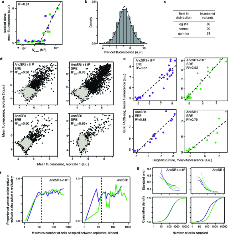
Figure 1 |. Diverse sequences and mechanisms can yield the derived DNA specificity.

a, The historical transition in DNA-binding specificity in steroid receptors occurred through 3 changes in the recognition helix (RH), which required permissive substitutions (11P)¹¹. We searched for other RH mutations (RH′) that could produce the derived function, before or after 11P. Each clade’s preferred DNA response element and RH protein sequence (residues 24–33) are shown; underlined, historically variable states. ERs, estrogen receptors; SRs, other steroid receptors. Reconstructed ancestral proteins are colored by response element preference. b, FACS-seq assay for steroid receptor DNA recognition. A library of 160,000 RH variants was cloned into yeast with ERE- or SRE-driven GFP reporters. Each variant’s activity was estimated by FACS and deep sequencing. c, GFP activation on ERE and SRE by each variant in the AncSR1+11P background. Purple dots, ERE-specific variants; green, SRE-specific; blue, promiscuous; black, non-functional; gray, stop-codon variants. Purple line, activity of AncSR1:EGKA on ERE; green line, AncSR1+11P:GSKV on SRE. d, Frequency of residues at each variable position among ERE- and SRE-specific variants; n, number in each class. Red, acidic; blue, basic; magenta, polar uncharged; black, large nonpolar; green, small nonpolar. Residues and numbers in AncSR1 and AncSR2 are shown. e,f, Diverse biochemical mechanisms for recognition of SRE (e) or ERE (f) by the historical derived RH (GSKV) and an alternative SRE-specific variant (KAAI). Contacts in structural models are shown between RH residues (circles) and DNA. Arrows, hydrogen bonds from donor to acceptor; dotted lines, non-bonded contacts. Red squares, unsatisfied bases that hydrogen-bond in EGKA-ERE. Only variable RH-DNA contacts are shown (see Extended Data Figure 4).

To characterize alternative ways by which SRE specificity could have evolved (Fig. 1a), we focused on the RH, the only portion of the protein that directly contacts the nucleotides that vary between ERE and SRE. We prepared a library that contains all 160,000 combinations of all 20 amino acids at four key sites in the RH – the three that historically shifted DNA specificity, plus a physically adjacent lysine that varies among the broader receptor superfamily (Fig. 1b). The library was constructed in AncSR1+11P, the genetic background that enabled the historical RH substitutions to alter DNA specificity. We engineered yeast reporter strains in which ERE or SRE drives expression of a fluorescent GFP reporter and showed that GFP activation directly relates to DNA affinity (Extended Data Fig. 1a)¹⁸. We transformed the library into each reporter and used FACS coupled to deep sequencing (FACS-seq) to quantify binding of each variant in the library to ERE or SRE (Extended Data Figs. 1, 2, 3, Extended Data Table 1). We classified genotypes as ERE-specific, SRE-specific, promiscuous, or inactive; results of all downstream analyses were robust to the specific classification criteria (Extended Data Table 2).

We found 828 new RH variants that are SRE-specific, binding SRE as well or better than the historical outcome and displaying no activity on ERE (Fig. 1c). These alternative SRE-specific genotypes employ amino acids with diverse biochemical characteristics (Fig. 1d), and they discriminate between SRE and ERE using different physical contacts (Figs. 1e, f, Extended Data Fig. 4). For example, the historical outcome (RH sequence GSKV) binds SRE in part by polar contacts from Lys28 to nucleotides A1 and G2, but the alternative outcome KAAI makes no polar contacts using residue 28, instead hydrogen-bonding from Lys25 to A1, G2, and the opposite-strand nucleotide T−3 (Fig. 1e). It also exhibits novel mechanisms of ERE-exclusion: whereas GSKV leaves the hydrogen bonding potential of C−3 unsatisfied, KAAI also leaves G2 and T4 unpaired, because Ala28 – unlike Lys28 of GSKV – cannot bond to G2, and Ile29 interferes with a hydrogen bond to T4 made by the conserved Arg33 residue (Fig. 1f, Extended Data Fig. 4c).

Figure 4 |. Effect of historical permissive substitutions is mediated by nonspecific increases in affinity.

a, Predicted SRE-binding affinity of SRE-specific variants that require 11P (orange, n=790) or do not (yellow, n=41) in AncSR1 (left) or AncSR2 (right). In each category, the median (bar), 95% confidence interval (notch), interquartile range (box), and range (whiskers) are shown. P-value, difference of medians (Wilcoxon rank-sum with continuity correction). b, Frequency of states at variable RH sites among SRE-specific variants in AncSR1 (left) or AncSR1+11P (right). Colors as in Fig. 1d. c, Biochemical determinants of SRE specificity in AncSR1 (top) and AncSR1+11P (bottom). A multiple logistic regression model predicts the probability that a variant is SRE-specific from the properties of the residues at each variable site: v, volume; h, hydrophobicity; i, isoelectric point; α, α-helix propensity. Colored boxes show best-fit model coefficients as the effect on classification odds per unit change in each property; *, significant difference between AncSR1 and AncSR1+11P (Z-test, P <0.05). d, The AncSR1+11P RH functional network. Yellow, variants that are functional without 11P; orange, variants that require 11P. e, For each RH genotype that does not require 11P, the number of single-mutant neighbors that became functional when 11P was introduced.

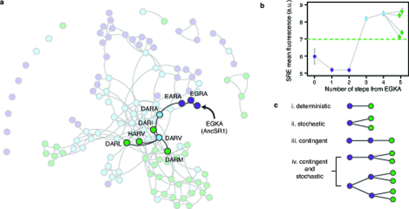
The historical outcome is therefore not unique in its genetic or biochemical mechanism of SRE specificity, but it might have been uniquely accessible from the ancestral RH. To investigate the distribution of functions across sequence space, we constructed a force-directed graph of functional RH variants (Fig. 2a). Each node represents a functional RH genotype, and edges connect nodes separated by one nonsynonymous nucleotide mutation (steps). The network contains clusters of densely interconnected variants that share distinguishing amino acid states, with epistasis and the structure of the genetic code separating the clusters. Although the vast majority of RH variants are nonfunctional, virtually all of the 1351 functional variants are part of a single connected network that can be traversed without visiting nonfunctional genotypes².

Figure 2 |. Evolvability of SRE specificity in an ancestral sequence space.

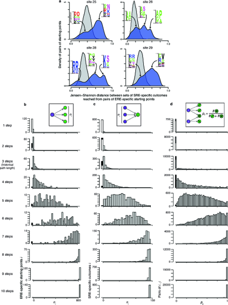
a, Force-directed graph shows the functional topology of the RH sequence space in AncSR1+11P. Nodes, all functional RH variants, colored by specificity as in Fig. 1c; yellow, SRE-specific variants accessible from EGKA in ≤3 mutational steps (the length of the historical trajectory). Edges, single nonsynonymous nucleotide mutations. Clusters (grey arcs) are labeled by their defining genetic features; x, variable sites within a cluster. Historical ancestral and derived RH genotypes are indicated. b, Distribution of ERE-specific nodes (starting points) by number of SRE-specific nodes (outcomes) reached in ≤3 steps. Black, starting points that reach zero outcomes because epistasis results in nonfunctional intermediates^7,8. c, Distribution of outcomes by number of starting points that reach it in ≤3 steps. Black, outcomes reached from zero starting points because of epistasis; white, because all starting points are >3 nonsynonymous mutations away. d, Distribution of pairs of starting points by the fraction of outcomes within ≤3 steps that are shared. Black, pairs with zero shared outcomes because of epistasis; white, because starting points are too far apart to reach the same genotypes; hatched, because no mutually accessible genotypes are SRE-specific.

The ancestral and derived RHs (EGKA and GSKV, respectively) are connected by a path of just three steps, whereas the most distant proteins in the network are 13 steps apart. From the ancestral starting point, GSKV is not uniquely accessible: 64 other SRE-specific RHs are accessible in three or fewer steps without passing through nonfunctional intermediates. Some of these alternative outcomes can be reached in just one or two steps, and these too exhibit biochemically diverse amino acid states (Extended Data Fig. 5a). If selection against too-tight or too-weak binding allows access only to genotypes with DNA affinity in a narrow range indistinguishable from the historical genotypes, there are still hundreds of alternative SRE-specific outcomes, many of which are easily accessible from the historical starting point (Extended Data Table 2, column E). Even when trajectories are allowed only if SRE affinity increases at every step – as would occur under positive selection for that function – there are numerous alternative SRE-specific genotypes with a nontrivial probability of evolving from the ancestral RH, and all of these are more likely than the historical outcome (Extended Data Fig. 5a,b,c). Taken together, these data indicate that the historical trajectory was not the only path, or even the shortest, from the ancestral RH to a derived protein that is SRE-specific.

Next, we asked whether the evolution of SRE specificity depended on the starting point within the large network of mutually accessible ERE-specific genotypes. All but 2 ERE-specific variants can get to SRE specificity without passing through nonfunctional intermediates (Fig. 2a), and more than 90% can do so by paths no longer than the historical trajectory (Fig. 2b). Evolution of the derived specificity per se was therefore not strongly dependent on the starting point. Whether any particular SRE-specific genotype would evolve, however, could be contingent on where in the network of ERE-specific variants an evolutionary trajectory begins. For each SRE-specific RH, we asked how many ERE-specific starting points could access it by a path no longer than the historical three-step trajectory (Fig. 2c). About one-third of possible SRE-specific genotypes are not easily reached from any possible starting point – some because the large diameter of the functional network means that the minimum genetic distance to the closest ERE-specific variant is more than three nonsynonymous mutations, and some because epistasis requires trajectories longer than the minimum genetic distance^7,8. Of the remaining SRE-specific variants, most (including the historical outcome GSKV) are readily accessible from just one or a few starting points, and even the most accessed outcome is easily reached from less than one-third of all possible starting points. As a result, most pairs of ERE-specific starting points reach entirely non-overlapping sets of SRE-specific outcomes (Fig. 2d), which contain distinct sets of amino acids (Extended Data Fig. 6a). The evidence for dependence on starting point persists when path lengths longer than the historical trajectory are considered (Extended Data Fig. 6b,c,d) and when alternate evolutionary models are applied (Extended Data Table 2). Taken together, these data indicate that the derived specificity for SRE could have evolved in many ways from AncSR1+11P, but the underlying genetic and biochemical form depended strongly on the starting RH genotype.

We next asked how the historical permissive substitutions affected the accessibility of the derived specificity and its dependence on starting point. We constructed and characterized the same four-site combinatorial RH library, this time in the AncSR1 background without 11P (Fig. 1a, Fig. 3a, Extended Data Fig. 1). Removing 11P dramatically reduces the number of functional variants (Fig. 3b) and the connectivity of the network (Fig. 3c). Unlike the AncSR1+11P sequence space, many functional variants in AncSR1 are isolated and therefore cannot be reached from most other genotypes without passing through nonfunctional intermediates. Still, most functional RHs – including the ancestral EGKA – are interconnected in the primary subnetwork, where many SRE-specific RHs are accessible. Therefore, although the historically derived RH genotype GSKV requires the historical permissive substitutions, other genotypes with the derived specificity could have evolved without 11P. But trajectories in the AncSR1 sequence space are more complex: the shortest path from the ancestral RH to any SRE-specific variant is 5 steps, all paths require permissive RH steps that do not enhance SRE activity, and all paths require promiscuous intermediate genotypes (Extended Data Fig. 7a,b). Thus, without the historical permissive substitutions, other permissive mutations would have been required for SRE specificity to evolve from the ancestral genotype.

Figure 3 |. Historical permissive substitutions enhanced evolvability of SRE specificity.

a, GFP activation on ERE and SRE by each RH variant in the AncSR1 background; colors as in Fig. 1c. b, Variants by functional class in the AncSR1 and AncSR1+11P backgrounds. c, Functional topology of the RH sequence space in AncSR1, represented as in Fig. 2a. d, Distribution of ERE-specific starting points by length of the shortest path to an SRE-specific outcome in AncSR1 (left) and AncSR1+11P (right). 11P reduce the shortest path length (P <10⁻¹², Wilcoxon rank-sum with continuity correction). e, For all connected starting points in AncSR1 (left) and AncSR1+11P (right), the shortest path(s) to SRE specificity classified by trajectory type: permissive (via ERE-specific intermediates), promiscuous (via promiscuous intermediates), both, or direct (one-step path without permissive or promiscuous intermediates). Starting points with paths in multiple categories contribute proportionally to each. Distributions differ between the networks (P <10⁻⁷, Chi-squared test).

The 11P substitutions enhanced the accessibility of SRE specificity not only from the ancestral genotype but from all ERE-specific starting points. Whereas virtually all starting points in the AncSR1+11P network could access at least one SRE-specific node without passing through nonfunctional intermediates, over a fourth of ERE-specific variants in AncSR1 have no path to the derived specificity, and those that can access SRE specificity require longer paths (Fig. 3d). Removing the historical permissive substitutions also increases the proportion of ERE-specific starting points that require a permissive step prior to acquiring SRE activity (Fig. 3e). And, unlike the AncSR1+11P network, every path from ancestral to derived specificity in AncSR1 must pass a promiscuous intermediate (Fig. 3e).

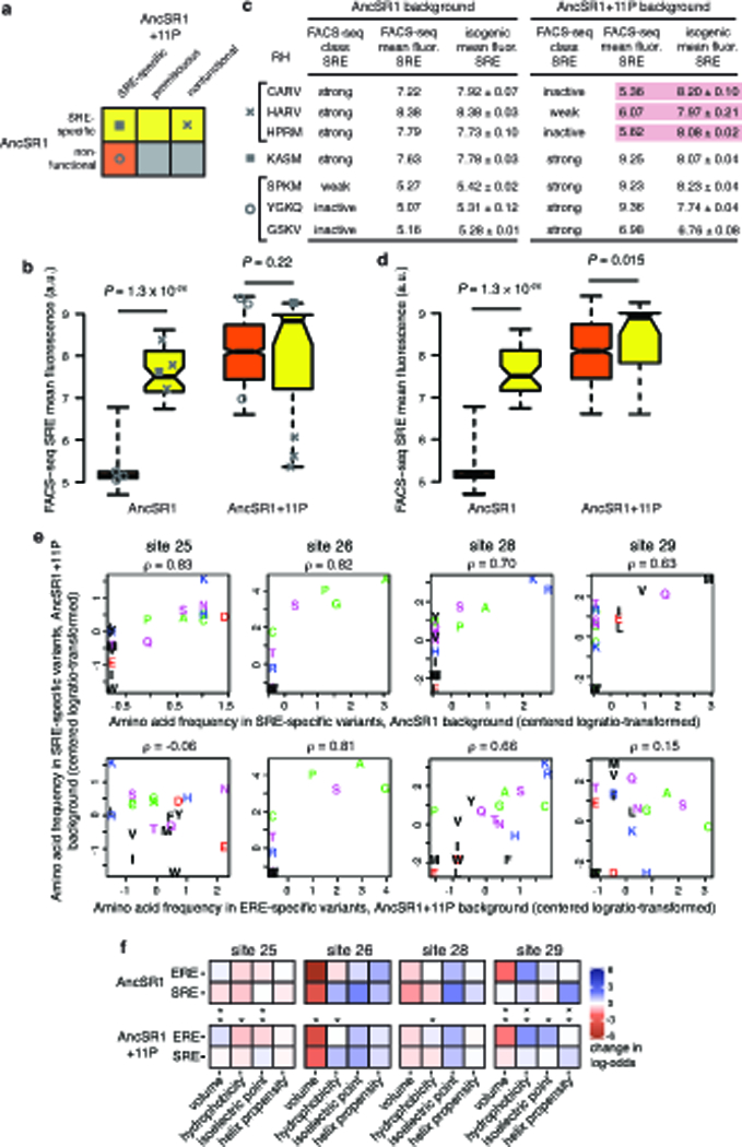
Finally, we investigated the mechanism by which the historical permissive substitutions enhanced the potential for evolution across the RH sequence space. 11P were broadly permissive, increasing the number of SRE-specific genotypes in the network by a factor of 20 (Fig. 3b). Previous work suggests that increases in protein stability sometimes mediate generalized permissive effects^20–23, but 11P have been shown not to increase the stability of AncSR1¹¹. We previously proposed that 11P permitted the historical RH substitutions by nonspecifically increasing affinity for both response elements¹¹, which would explain the broadly permissive effect of 11P on many RH genotypes. This hypothesis makes four testable predictions. First, RH variants that do not depend on 11P to yield SRE specificity should have greater SRE affinity than those that require 11P, whether or not 11P are present; we compared the predicted affinity and FACS-seq mean fluorescence of all 11P-independent and 11P-dependent SRE-specific variants and found that this prediction holds true (Fig. 4a, Extended Data Fig. 8a-d). Second, 11P should not change the genetic determinants of binding within the RH; as predicted, the most enriched residues among SRE-specific variants do not change between the two networks, but 11P weakens the preference for some tolerated states over others (Fig. 4b, Extended Data Fig. 8e). Third, 11P should not change the biochemical mechanisms by which the RH confers specificity, a prediction we tested by identifying the biochemical properties at each RH site that predict specificity for ERE and SRE (Extended Data Fig. 8f): we found that the determinants of SRE specificity are not dramatically altered by 11P (Fig. 4c). Fourth, if 11P nonspecifically enhance affinity by all RHs, they should add new functional genotypes across sequence space; we found that the set of variants permitted by 11P are not localized to some region of the network but instead surround the sparser set of variants that functioned independently of 11P (Fig. 4d,e). As a result, 11P’s nonspecific effect on affinity enhanced the connectivity of the ancestral sequence network, increasing the number and reducing the length and complexity of paths from ERE to SRE.

Our results shed light on the roles of determinism and chance in protein evolution^1,3,22,24. The primary deterministic force is natural selection, which drives the evolution of forms that optimize fitness. Chance appears in two non-exclusive ways: as historical contingency – when the accessibility of some outcome depends on prior events that cannot be driven by selection for that outcome – and as stochasticity – when there are paths to numerous possible genotypes of similar function, and which one is realized is random (Extended Data Fig. 7c)¹. Previous work has shown that historical function-switching substitutions in some proteins were contingent on prior permissive mutations^{11,20,25–27}, but the overall roles of chance and determinism in the evolution of a new function can be understood only by characterizing other ways that the function could have evolved. Our results point to strong stochasticity and contingency in the many histories by which SRE specificity could have evolved. Hundreds of genotypes encoding SRE specificity were accessible from AncSR1, but selection for that function alone could not have deterministically driven evolution down any of those paths, because all were contingent on permissive mutations – either the historical 11P or alternative permissive mutations within the RH. Which particular permissive mutations happened to occur determined which SRE-specific genotypes then became accessible. Further, given some permissive set of first steps, paths to numerous SRE-specific genotypes typically become available. Thus, evolution of any particular SRE-specific outcome – including the one that evolved during history – is contingent on the initial stochastic acquisition of some set of permissive mutations, followed by the subsequent stochastic realization of one of many possible ways to encode the derived function.

Some aspects of real and counterfactual history cannot be reconstructed, but our conclusions are likely to be robust to major forms of uncertainty. For example, the precise probability of any trajectory depends on population size and on the relationship between molecular function and fitness, but neither of these is known. Still, we found that contingency and stochasticity were important not only under scenarios that emphasize purifying selection and drift, but also under those that favor determinism, such as when selection drives continuous enhancement of the derived function or allows affinity within only a narrow range. Second, sequence space is so vast that we could explore only a limited portion. But contingency and stochasticity are likely to remain important when larger regions are considered. If these unexplored regions contain additional trajectories to SRE-specific outcomes, then the role of stochasticity in the choice among options would be even more important. Morevoer, contingency on starting point arising from the distribution of SRE-specific genotypes across sequence space would persist even if new potential outcomes were discovered, and it would be magnified if those outcomes were even more distant than those we characterized. Finally, the dependence on permissive mutations that we observed would be eliminated only if there is a mutation at some other site that could somehow confer SRE activity on AncSR1 in a single step; this seems implausible, because all other residues are distant from the variable bases.

Despite the abundance of accessible SRE-specific genotypes near the ancestral and derived RHs (Extended Data Fig. 5d,e), the genotype that historically evolved is conserved among present-day descendants. It is possible that some unknown property made this sequence selectively superior to the many genotypes that are at least as effective at recognizing SRE and excluding ERE. But it could also be conserved because of factors that accumulated after it evolved. For example, a substitution can become epistatically entrenched by subsequent restrictive substitutions at other sequence sites^28,29. A transcription factor’s sequence may also become pleiotropically entrenched by subsequent mutations in the ensemble of response elements it binds³⁰. If one of the many alternative SRE-specific outcomes evolved from the ancestral protein by chance, it too could have been subsequently locked in, yielding conservation and the illusion that it evolved deterministically. The singularity of the present seems to rationalize the past. History leaves no trace of the many roads it did not take, or of the possibility that evolution turned out as it did for no good reason at all.

Methods

Construction and validation of a yeast assay for steroid receptor DNA-binding domain function.

All work was performed in S. cerevisiae strain K20 (CEN.PK 102–5B, URA3^-, HIS3^-, LEU^-)³¹. Oligonucleotide sequences used for cloning and sequencing are included in Supplementary Table 1. We constructed yeast reporter strains containing yEGFP under the control of a minimal CYC1 promoter with two upstream ERE or SRE palindromes, integrated into the ADE2 locus³¹. Colony PCR and Sanger sequencing confirmed correct integration of the ERE₂-yEGFP or SRE₂-yEGFP reporter. An additional 20 μg/mL adenine hemisulfate was added to all media to ameliorate ADE2 disruption.

The yeast expression plasmid pTNS33 contains the AncSR1 DNA-binding domain (DBD, GenBank AJC02122.1)¹¹ with an N-terminal SV40 nuclear localization sequence and Gal4 Activation Domain (AD) connected by a 9-residue linker (IQQGGSGGS). Expression of the AD-DBD fusion protein is controlled by the galactose-inducible GAL1 promoter, in the background of the pRS413 plasmid³² containing a HIS selection marker. We assembled pTNS33 by yeast homologous recombination using the LiAc/ssDNA/PEG method³³, selecting for growth on SC-His plates with 2% Dextrose (+D). We confirmed correct plasmid assembly via Sanger sequencing.

To validate the ERE₂-yEGFP and SRE₂-yEGFP reporters, a selection of previously assayed DBDs spanning a range of DNA-binding affinities^11,12 were cloned into the pTNS33 background and transformed into each yeast reporter strain. Individual colonies were inoculated in 3mL SC-His with 2% raffinose (+R), and incubated for 16 hours at 30 ºC 225 rpm in an orbital shaker incubator. Cells were back-diluted to 0.25 OD₆₀₀ in SC-His with 2% galactose (+G) to induce DBD expression and grown for an additional 24 hours. Cells were pelleted and suspended to 1 OD₆₀₀ in 1× TBS. We analyzed 10,000 cells of each genotype by flow cytometry on a BD LSR-Fortessa 4–15, with 488 nm excitation and 530 nm emission. We used gates drawn empirically on FSC/SSC and FSC-H/FSC-A scatter plots (e.g. Extended Data Fig. 2) to isolate a homogeneous cell population, from which we determined the mean per-cell green fluorescence. The relationship between mean GFP activation and previously measured binding affinities was fit to a segmented-linear relationship in R³⁴ with the ‘segmented’ package³⁵.

Library generation.

AncSR1 and AncSR1+11P RH libraries were constructed by synthesizing pools of oligonucleotides containing degenerate NNK codons at four variable sites in the recognition helix and inserting these into coding sequences for the previously reconstructed AncSR1 DBD or the AncSR1+11P DBD, which contains the 11 previously identified historical permissive mutations¹¹. These libraries encode all combinations of all 20 amino acids at the three RH sites that changed during the historical evolution of SRE specificity (sites 25, 26, and 29) and at the adjacent position (site 28), which physically interacts with the substituted residues¹¹ and varies among the broader nuclear receptor superfamily³⁶. Each RH library contains 1,048,576 genetic variants, encoding 160,000 full-length proteins and 34,481 stop-codon-containing variants. To construct the libraries, 53-nt single-stranded DNA oligonucleotides were synthesized (DNA2.0, Newark, California), containing variable RH sites and invariant flanking sequence identical to the respective plasmid sequences (Supplementary Table 1). Oligonucleotide pools were converted to dsDNA by primer extension with Klenow polymerase and purified on a Qiagen MinElute column. Yeast expression plasmids containing AncSR1 or AncSR1+11P were modified by site-directed mutagenesis to introduce EcoRI and NcoI sites, which were cut to excise the native RH and linearize the vector to receive the oligonucleotide pool. Plasmid libraries were assembled via Gibson Assembly, incubating 0.56 pmol gel-purified linear vector, 8.4 pmol oligonucleotide pool, and 120 μL 2× GA Master Mix (NEB) at 50 ºC for 1 hr. Assembled libraries were purified over DNA Clean & Concentrator columns (Zymo) and transformed into electrocompetent NEB5α E. coli cells with a 2.5 kV electroporation pulse in 0.2 mm gap cuvettes. Aliquots of cells were serially diluted and plated on LB+carbenicillin to estimate transformation efficiencies. Remaining cells were grown overnight in LB+carbenicillin, and plasmids were harvested using the GenElute Midiprep plasmid purification kit. For both the AncSR1 and AncSR1+11P RH libraries, we obtained at least 20 times more transformants than the effective size of the library (Extended Data Table 1).

Each RH library (AncSR1 and AncSR1+11P) was independently transformed twice into each yeast reporter strain (ERE and SRE) for replicate FACS-seq analyses. We followed a yeast electroporation protocol³⁷, scaled up for 10 times the number of cells and a total of 120 μg of library plasmid in 600 μL H₂O. An aliquot of cells was serially diluted and plated on SC-His+D to estimate transformation yield, which averaged 1.25×10⁷ cfus across the 8 transformations (Extended Data Table 1). The remaining cells were grown to saturation in 500 mL SC-His+D. Consistent with previous observations³⁸, we observed that seven out of eight colonies post-transformation were multiple-vector transformants. We performed an additional passage, at which point multiple-vector clones were detected at less than one in eight colonies. A total of five passages occur prior to quantification (see below), so multiple vector transformants are expected to occur at a frequency no greater than 0.007 in the library. Furthermore, if our conclusion that there are many functional RH variants were caused by false positives due to co-transformation of nonfunctional genotypes with functional ones, this would result in stop-codon-containing variants being classified as functional, but this was never observed. Passaged yeast library aliquots of 3×10⁹ cells were flash frozen in liquid nitrogen and stored at −80 ºC as 25% glycerol stocks.

Library induction and FACS.

Yeast library aliquots were thawed on ice, added to 500 mL SC-His+D, and grown for 12 hours at 30 ºC 225 rpm. Cells were diluted to 0.25 OD₆₀₀ in 500 mL SC-His+R, and grown for an additional 12 hrs at 30 ºC 225 rpm. Cells were then diluted to 0.25 OD₆₀₀ in 200 mL SC-His+G to induce DBD expression, and grown for 24 hrs at 30 ºC 225 rpm. Induced cells were spun at 3,000 g for 5 min, suspended to 3×10⁷ cells/mL in 1× TBS, passed through a 40 μm nylon cell strainer, and stored on ice for sorting. Alongside each library induction, we induced isogenic controls expressing known DBDs according to the same protocol but at 3 mL volumes.

Each library was sorted into 4 bins on a BD FACSAria II. Initial gates were drawn to isolate homogenous cells and exclude doublets, using SSC/FSC and FSC-H/FSC-A scatterplots (Extended Data Fig. 2). We assigned sort gate boundaries to the AncSR1+11P/SRE library to correspond to the observed mean fluorescence of a stop-codon-containing variant, of AncSR1+11P:GSKV, and AncSR1+11P:GGKA, the variant with the highest previously known activation; these gates yielded four bins that captured 45%, 45%, 9.5%, and 0.5% of the library population, respectively. Gates for other libraries were assigned to yield the same bin sizes. To calibrate the arbitrary-unit fluorescence scales of sorting experiments conducted on different days, we transformed fluorescence values by a linear model fit to the relationship between mean fluorescence of reference isogenic cultures induced and analyzed in parallel to each library sorting experiment. Cells were sorted into SC-His+D with 34 μg/mL chloramphenicol to prevent bacterial contamination and stored on ice until ~10⁸ cells were sorted. An aliquot of cells sorted into each bin was serially diluted and plated to estimate cfu recovery (Extended Data Table 1). Remaining cells were suspended to an estimated 200,000 cells/mL in SC-His+D+chloramphenicol, and grown for 16 hours at 30 ºC 225 rpm. Plasmids were extracted from each outgrowth according to the protocol of Fowler et al.³⁹, which was scaled up 16-fold for bins 1 and 2, 8-fold for bin 3, and 3-fold for bin 4 to avoid bottlenecks. Extracted plasmids were estimated to be present at a concentration of 2×10⁶ plasmids/μL by comparing bacterial transformation efficiencies of yeast-extracted plasmid to pUC19 and bacterial-purified plasmid standards.

Sequencing and processing.

We used PCR to amplify the variable RH region from post-sort plasmid aliquots; primers appended in-line barcodes⁴⁰ to identify the experiment and sort bin, along with binding sites for sequencing primers and Illumina flow cell adapter sequences (Supplementary Table 1). Barcodes were of different lengths to stagger reads across clusters and were assigned to bins to optimize the distribution of base calls at each position during the initial rounds of sequencing. Multiple barcodes were used for bins 1 and 2, which contained the majority of cells. For each bin-barcode combination, PCR was conducted in 8 replicate 50-μL aliquots, with 10 μL of plasmid template, 10 μL 5× HF buffer, 1 μL 10 mM dNTPs, 2.5 μL 10 μM forward and reverse primer, and 0.5 μL Phusion polymerase per reaction. PCRs were assembled on ice, transferred to a thermocycler block preheated to 98 ºC, and subjected to 20 PCR cycles with 60 ºC annealing. PCRs were gel-purified, quantified via BioAnalyzer and qPCR, and then pooled for sequencing according to the relative numbers of cells acquired in each bin. Single-end 50bp reads spanning the barcode and RH sequence were acquired on an Illumina HiSeq2500.

We discarded sequence reads with an average Phred score <30 and sequences that did not perfectly match the barcode and invariant portion of the template. Reads were demultiplexed by barcode and further processed using tools from the FASTX-Toolkit (http://hannonlab.cshl.edu/fastx_toolkit/). RH variants with inconsistent read numbers between barcodes in the same bin were considered uncharacterized for that entire experiment. This procedure yielded filtered read counts in each sort bin greater than the number of cells sorted into that bin (Extended Data Table 1). To estimate the number of cells of a genotype that were sorted into a bin, we divided the number of sequence reads of a genotype in a bin by the average number of reads per cell in that bin.

Estimating mean fluorescence and standard error.

We estimated the mean fluorescence of each variant in the library from the distribution of its reads across fluorescence sort bins using a maximum likelihood approach⁴¹. We first assessed the fit of various distributions to the observed per-cell fluorescence of a series of isogenic cultures of different RH genotypes analyzed in isolation via flow cytometry, and found the logistic distribution to have the best fit by AIC (Extended Data Fig. 1b,c). We then used the ‘fitdistrplus’⁴² package in R to find the maximum likelihood mean fluorescence for each library variant given its distribution of cell counts across sort bins, the fluorescence boundaries of those bins, and the logistic distribution; this approach explicitly takes into account the fact that the fluorescence of a cell within a sort bin is not precisely measured and has been shown to be an unbiased approach for estimating underlying activities in FACS-seq analyses⁴¹. Estimates of mean fluorescence from the FACS-seq library characterization were compared between independent replicates (Extended Data Fig. 1d). Interval-censored per-cell observations from the two independent replicates were then pooled, and the maximum likelihood mean fluorescence for each variant estimated from this pooled data. These final estimates were compared to fluorescence observed directly for isogenic cultures of randomly selected clones from each library, which were isolated post-sort, genotyped, re-induced in isogenic cultures and analyzed via flow cytometry according to the protocol above (Extended Data Fig. 1e).

We estimated the standard error of mean fluorescence (SEM) for genotypes based on their depth of coverage (number of cells sampled) in two ways. First, we estimated SEMs from stop-codon-containing variants in each library by grouping them according to their depth of coverage and calculating the standard deviation of the sampling distribution of estimated mean fluorescence for variants in each group. Second, we leveraged variability in the mean fluorescence estimates from the two replicate FACS-seq experiments for each library: using coding variants for which the number of cells sampled between replicates is within 20% of each other, we calculated the difference between the estimate of mean fluorescence from the pooled data and the estimates from each of the two replicates, grouped variants by their average depth of coverage for the two replicates, and calculated the standard deviation of the distribution of differences for each group. Every variant in the library was then assigned the SEM for the appropriate coverage depth group. These two approaches yielded a similar relationship between SEM and sampling depth, but the second approach estimated higher SEMs at higher coverage depths (Extended Data Fig. 1g); to be conservative, we therefore used the second approach for further analyses.

Classifying strength of activation on each response element.

We used mean fluorescence estimates to classify the strength with which each library variant binds to ERE and SRE using nonparametric comparisons to distributions of reference genotypes. A variant was classified as active on a response element if its mean fluorescence was significantly greater than that of stop-codon-containing variants contained in the library: for each variant, the P-value for the null hypothesis that a variant is inactive was calculated as the proportion of stop-codon-containing variants of similar sampling depth with greater mean fluorescence than that of the variant of interest; variants were labeled “active” if the null hypothesis could be rejected at a 5% false discovery rate (using the Benjamini-Hochberg procedure) or “inactive” if the null hypothesis could not be rejected.

Each active variant was then subclassified as a weak or strong activator by comparing its mean fluorescence to that of the relevant ancestral genotypes (AncSR1:EGKA on ERE, or AncSR1+11P:GSKV on SRE). Specifically, for each active variant we performed a test of noninferiority within an equivalence margin of 20% of the range between the average mean fluorescence of stop-codon-containing variants and the mean fluorescence of the ancestral reference. This test compares the mean fluorescence of a variant of interest to the fluorescence of cells with the relevant ancestral genotype, shifted to 80% of the range between the mean of stop-codon-containing variants and the ancestral reference. To determine whether a variant’s fluorescence is greater than this shifted ancestral reference, we generated 10,000 bootstrap replicates from the shifted distribution of ancestral cellular fluorescence, with replicate size of similar sampling depth to the variant of interest; the mean fluorescence of each bootstrap replicate was calculated using the FACS gates and maximum likelihood procedure described above. The P-value for the null hypothesis that a variant is a weak activator was calculated as the proportion of bootstrap replicates with fluorescence greater than that of the variant of interest; variants were classified as “strong” if the null hypothesis could be rejected at a 5% false discovery rate (using the Benjamini-Hochberg procedure) or “weak” if the null hypothesis could not be rejected. AncSR1:EGKA was represented by relatively few cells in the ERE library, resulting in an artificially low mean fluorescence determined by FACS-seq and a “weak” classification, so it was manually classified as a strong activator on ERE by definition. For library classifications, we determined the reference activity of AncSR1:EGKA on ERE from an isogenic culture analyzed in parallel to library sorts. Using the lower FACS-seq mean fluorescence measurement as the reference activity for this genotype does not alter our conclusions (Extended Data Table 2, column A).

Extrapolation to missing genotypes.

Classification of variants that are rare in the library may not be reliable. We examined how agreement in classification between FACS-seq replicates is affected by sampling depth, and we found that the probability that a variant is classified as positive in one replicate if it is classified as positive in the other depends on sampling depth below 15 cells (Extended Data Fig. 1f). We therefore considered variants with 15 or fewer cells to be experimentally undetermined, accounting for 2.0% to 8.8% of all variants across the four DBD/response element combinations (Extended Data Table 1). To predict the classification of these variants, we used a continuation ratio ordinal logistic regression model that predicts the probability that a variant is strong, weak, or inactive from its genotype, trained on the empirical classification of all the determined genotypes in the library. We modeled amino acid states as potentially contributing first-order main effects (20 states × 4 positions = 80 parameters) and pairwise epistatic effects (₄C₂ × 20² = 2,400 parameters). We fit these models to the observed classifications in each library using a coordinate-descent fitting algorithm with L₁ penalization, as implemented in the ‘glmnetcr’ package⁴³ in R. We used 10-fold cross validation to determine the quality of model predictions and to select the penalization parameter λ. We set λ = 10⁻⁵ to obtain a high true positive rate without compromising the positive predictive value (Extended Data Fig. 3).

Classifying response element specificity.

The specificity of each variant was determined from its functional classification on ERE and SRE. ERE-specific variants are strong on ERE and inactive on SRE; SRE-specific variants are strong on SRE and inactive on ERE; promiscuous variants are strong on one response element and strong or weak on the other; and nonfunctional variants are not strong on either response element. The false positive rate was very low, with no stop-codon-containing variants classified as functional. AncSR1+11P:EGKA is classified as promiscuous, because it has very strong ERE activity and SRE activity that is very weak but statistically distinguishable from background, consistent with previous observations¹¹.

A small number of RH variants were unexpectedly inferred to be functional in AncSR1 but nonfunctional in AncSR1+11P (Extended Data Fig. 8a-c). To validate this observation, we re-cloned the three SRE-specific variants with the largest reduction in fluorescence when 11P were included (CARV, HARV, HPRM) and assessed their SRE activation in the AncSR1 and AncSR1+11P backgrounds in isogenic cultures via flow cytometry; for comparison, we also validated a putatively 11P-independent genotype (KASM) and two 11P-dependent variants (SPKM, YGKQ), alongside GSKV for reference. Inductions were conducted in triplicate, each from an independent transformant. Classifications of the three comparison genotypes were all confirmed; however, the three genotypes that were putatively restricted by 11P showed no reduction in fluorescence in this assay, indicating that they were falsely classified as nonfunctional in the AncSR1+11P FACS-seq assay (Extended Data Fig. 8c). Notably, the predictive logistic regression correctly predicts that these three variants are strong SRE-binders in the AncSR1+11P background. These three variants manifested strong growth defects in the AncSR1+11P background, even in the ERE strain in which they do not activate GFP expression.

Robustness of results to classification method.

We tested the robustness of our conclusions to alternative methods for classifying variants as functional. These include: (A) using the internal library AncSR1:EGKA mean fluorescence estimated by FACS-seq as the reference level of AncSR1 activation on ERE; (B) increasing the margin of equivalence to 50% of the activity difference between ancestral and stop-codon-containing variants; (C) classifying any active variant (weak or strong) as functional; (D) using the 80% mark of the range from stop-codon-containing to ancestral variants as a hard threshold rather than a null hypothesis for statistical testing; (E) defining functional variants as between 80% and 120% of the ancestral activity, so that extremely strong binders are classified as nonfunctional; (F) using predicted classifications for all variants, with experimental classifications used only to train predictive models; (G) using no predicted classifications, and labeling all undetermined genotypes as nonfunctional; (H) using for each variant the strongest functional class as predicted or determined by experiment; (I) using the experimental classification for a variant only if it was identical between replicates and predicting all others; (J) and using the per-variant estimates of the standard error of mean fluorescence based on coverage depth to calculate a P-value that a variant is inactive or weakly active given a normal distribution, rejecting each null hypothesis at a 5% FDR as above. When appropriate, ordinal logistic regression models were re-trained to predict missing genotypes under each scheme. These alterations made no qualitative differences to our conclusions (Extended Data Table 2).

Network construction and trajectories through sequence space.

Network representations of functional RH variants in the AncSR1 and AncSR1+11P backgrounds were constructed using the R package ‘rgexf’⁴⁴ and the network visualization program Gephi⁴⁵. Nodes representing RH variants were connected by edges if any genetic encoding of their protein-coding sequences could be interconverted with a single nucleotide mutation given the standard genetic code. The network was represented as a force-directed graph, which clusters nodes in two-dimensional space based on connectivity: nodes tend to repel each other, but each edge between connected nodes provides an attractive force; in the “equilibrium” layout, sets of densely interconnected nodes tend to cluster to the exclusion of less connected nodes. Force-directed graph layouts were constructed with the ForceAtlas2 method in LinLog mode, Gravity 1.0 and Scaling 0.8 (AncSR1) or 0.125 (AncSR1+11P).

We used the ‘igraph’⁴⁶ package in R to characterize the set of paths between functional nodes. A step was defined as a nonsynonymous nucleotide mutation between two functional variants; synonymous mutations within a single node were not considered as contributing to trajectory length. The graph was directed, so that trajectories can proceed from ERE to SRE specificity directly or via a promiscuous intermediate; nonfunctional intermediates² and functional reversions were not allowed, but “neutral” steps within a functional class were allowed. Epistasis was inferred when the shortest path between two nodes was longer than the minimum genetic distance between genotypes^7,8; epistasis may arise because the state at one site specifically modulates the functional effect of some state at another site or because of nonlinearity in the genotype-phenotype map⁴⁷, such as the threshold we used to classify variants as functional.

The distribution of shortest path length to SRE specificity from ERE-specific starting points in the AncSR1 and AncSR1+11P networks was compared via a Wilcoxon rank sum test with continuity correction, as observations were not normally distributed. The number of ERE-specific starting points in each network that require permissive steps and/or promiscuous intermediates on their shortest path to SRE specificity was compared via a Chi-squared test. All categories had an expected value of 5 or greater.

To compare genotypic states among outcomes reached from different ERE-specific starting points, we calculated the frequency distribution of amino acid states at each sequence site for the set of outcomes reached from each starting point; we then calculated the Jensen-Shannon (J-S) distance between these distributions for pairs of starting points. To capture a true amino acid state distribution across outcomes, we only considered ERE-specific starting points that access at least 15 outcomes (the median across all ERE-specific starting points). We compared these observed J-S distances to a null expectation of J-S distances in the absence of structure in sequence space, in which we randomly sampled two sets of variants from all possible SRE-specific outcomes according to the same sample sizes used in each real comparison, and calculated the J-S distance between these randomly sampled distributions.

We also considered a regime in which SRE-binding affinity is under strong selection, such that SRE-binding affinity is required to increase with each step; such a scenario has a strong potential to make evolution deterministically favor a single outcome. In this scheme, a step from one genotype to a neighbor was allowed only if the lower bound of the 90% confidence interval of the neighbor’s mean SRE fluorescence, estimated from its mean and SEM, was greater than the upper bound of the confidence interval of the starting genotype (indicating P < 0.02, ref. 48). We then calculated the probability of each accessible trajectory using two previously described models⁸: in the equal fixation model, any step that enhances SRE affinity from a particular node is equally likely to occur; in the correlated fixation model, the probability that an SRE-affinity-enhancing step occurs is directly proportional to the degree to which it increases SRE mean fluorescence, relative to the other SRE enhancing steps available from the given node.

Structural modeling and predictions of RE-binding affinity.

We used FoldX⁴⁹ to predict the affinity to SRE of all RH variants that were 11P-dependent (SRE-specific in the AncSR1+11P background and nonfunctional in AncSR1), or 11P-independent (SRE-specific in AncSR1; Extended Data Fig. 8a). For structure-based affinity prediction, we used the crystal structures of the AncSR1 DBD bound to ERE (PDB 4OLN) and the AncSR2 DBD bound to SRE (PDB 4OOR) as starting points, with crystallographic waters and non-zinc ions removed. We removed chains E, F, K and L from the 4OOR structure. We used the RepairPDB function to optimize both DBD structures according to the FoldX force field, and we used the BuildModel function to mutate the AncSR1/ERE structure to AncSR1:GSKV/SRE. The BuildModel function was then used to model each SRE-specific RH variant in complex with SRE on each of the AncSR1 and AncSR2 DBD structures, and the AnalyzeComplex function was used to predict the total DNA-binding energy of each protein variant with SRE. The predicted binding energies of 11P-dependent and 11P-independent variants were compared using a nonparametric Wilcoxon rank sum test with continuity correction, as data were not normally distributed. This test was conducted independently for energies predicted using the AncSR1 and AncSR2 structures. To compare these same groups as directly estimated in FACS-seq, a Wilcoxon rank sum test with continuity correction was used, as data were not normally distributed.

To characterize the diversity in biochemical mechanisms of SRE specificity, we analyzed FoldX models of the 10 most active SRE-specific variants that were identified in our AncSR1+11P FACS-seq experiment. We modeled binding to SRE using the AncSR2/SRE structure as described above and binding to ERE using the crystal structure of the AncSR2:EGKA DBD bound to ERE (4OND), with water and non-zinc ions removed and optimized using the RepairPDB function. To illustrate protein-DNA contacts made in each structural model, we used NUCPLOT⁵⁰ to identify all hydrogen bonds with distance ≤3.35Å between non-hydrogen atoms and non-bonded packing contacts ≤3.90Å. Summary figures display the union of contacts made by a residue in either of the half sites of the response element palindrome; we only illustrate residues whose contacts vary among the analyzed structures.

To ensure structural inferences converge, we built each SRE- and ERE-bound FoldX model a second time. We observed convergence in all polar contacts (and absence thereof in ERE structures) illustrated in Fig. 1 and Extended Data Fig. 4. Only several non-bonded contacts were not replicated: I29/T–4 in KAAI/SRE; Q29/A4 and Q29/T–4 in YGKQ/SRE; M29/T–3 in KSAM/SRE; and K25/G2 and K25/T–3 in KASM/SRE. To determine whether electrostatic clashes in ERE-bound structures could be satisfied by bridged water molecules⁵¹, models were built again using the BuildModel function with predicted waters. In some cases (GGRT, YGKQ, DSKM, CGRV), but not all (GSKV, KAAI, PAKE, KSAM, DPKQ, SAKE, KASM), polar groups on ERE that were not satisfied by direct interaction with protein side chains are predicted to be satisfied by water bridges between protein and DNA.

Biochemical determinants of RE-binding specificity.

Logos illustrating the frequency with which each amino acid state is found at each position among variants of a functional class were constructed using WebLogo⁵². Since our sequence space is combinatorially complete (all 160,000 genotypes are classified, either by FACS-seq or via prediction), the logo plots do not need to be normalized by background input frequencies. To evaluate similarity of the frequency profiles between classes of variants, the frequency of each amino acid state in a class was centered logratio-transformed, the appropriate transformation before computing correlations among compositional data; a pseudocount of one was added to the number of observations of each amino acid to allow log-transformation of states observed zero times. The Spearman rank correlation coefficient was computed for the correlation between functional classes.

To identify the biochemical properties of amino acids that contribute to DNA specificity, we developed a multiple logistic regression model that describes the probability that an RH variant specifically binds a response element as a function of the biochemical properties of the amino acid states at each of its four variable RH positions. The model includes four properties (hydrophobicity, volume, isoelectric point, and α-helix propensity), with the values for each amino acid’s properties from ref. 53, which we then centered and standardized; the effect of a unit change in each property at each site on the log-odds of being a specific binder is reflected in a model coefficient, which represent the model’s free parameters. We used R to find the values of these coefficients that best fit the observed classifications for each DBD/RE combination. Differences in the contribution of a property to specificity were identified if its associated coefficients in two models differed by a Z-test (P<0.05 with no correction for multiple testing)⁵⁴.

Data and code availability.

Raw sequencing data were deposited to the NCBI SRA under BioProject number PRJNA362734. Processed data and scripts to reproduce analyses are available at github.com/JoeThorntonLab/nature-2017_RH-scanning. A list of all RH sequences and their specificity classifications as used in the text is available in Supplementary Table 2.

Extended Data

Extended Data Figure 1 |. Design and validation of a yeast FACS-seq assay for steroid receptor DNA-binding function.

a, GFP activation in ERE (purple) and SRE (green) yeast reporters correlates with previously measured protein-DNA binding^11,12. Asterisk, stop-codon-containing variant. Dashed line, best fit segmented-linear relationship between GFP activation and log₁₀(K_a,mac) b, Histogram of the per-cell green fluorescence for AncSR1 on ERE measured via flow cytometry, fit to a logistic distribution (dashed line). c, Distributions that provide the best fit to flow cytometry data for isogenic cultures of 101 DBD variants, using Akaike Information Criterion (AIC). d, Comparisons of mean fluorescence estimates between FACS-seq replicates of each protein/response element combination. Black points, coding RH variants; light gray, stop-codon-containing variants. R²_pos, squared Pearson correlation coefficient for variants with mean fluorescence significantly higher than stop-codon-containing variants in either or both replicates. e, Comparisons between mean fluorescence as determined in FACS-seq and via flow cytometry analysis of isogenic cultures for a random selection of clones from each library. Dashed line, best-fit linear regression. f, Robustness of classification to sampling depth. Variants were binned according to the minimum number of cells with which they were sampled in either replicate. Below 15 cells sampled (dashed line), the probability that a variant called active in one replicate was also called active in the other is dependent on sampling depth; to minimize errors due to sampling depth, we eliminated as “undetermined” all variants with less than 15 cells sampled after pooling replicates. g, Standard error of mean fluorescence estimates (SEM) in each library as a function of sampling depth. Top plots show for each background, the relationship between SEM and sampling depth for ERE (purple) and SRE (green) libraries, as estimated from the sampling distribution of stop-codon-containing variants (dotted lines) or variability in mean fluorescence estimates between replicates (solid lines). Bottom panels show the cumulative fraction of coding variants in each library that have a certain number of cells sampled in the pooled data.

Extended Data Figure 2 |. Representative FACS gates for library sorting.

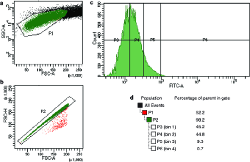
a, A scatterplot of side-angle scattering (SSC-A) and forward-angle scattering (FSC-A) selects for a homogenous cell population (P1). b, A scatterplot of the height of the per-cell forward scatter peak (FSC-H) and the integrated area of this peak (FSC-A) excludes events where multiple cells pass through the detector simultaneously (P2). c, Final sort bins (P3 – P6) are drawn on the distribution of green fluorescence (FITC-A). d, Table showing the hierarchical parentage of sort gates and the percentage of events that fall in each bin.

Extended Data Figure 3 |. Models to predict the function of missing genotypes.

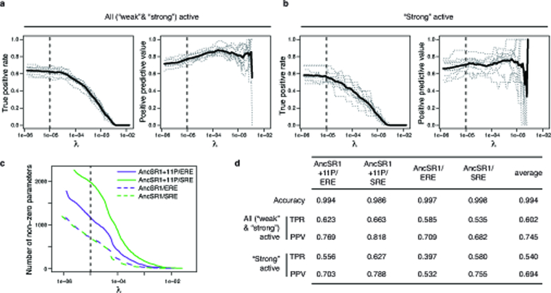
For each protein/response element combination, a continuation ratio ordinal logistic regression model was constructed to predict the functional class of a variant as a function of its four RH amino acid states, including possible first order main effects and second order pairwise epistatic effects. 10-fold cross-validation was used to select the penalization parameter λ and evaluate performance. a,b, True positive rate (left, TPR, the proportion of experimental positives that are predicted positive) and positive predictive value (right, PPV, the proportion of predicted positives that are experimentally positive) are shown as a function of λ for AncSR1+11P on ERE. Classifications were evaluated for (a) all active (weak and strong) versus inactive variants and (b) strong active versus weak active and inactive variants. Gray dotted lines, cross-validation replicates; solid line, mean. Dashed line shows the chosen value of λ = 10⁻⁵; as λ continues to decrease beyond λ = 10⁻⁵, TPR plateaus but PPV continues to decline. c, The number of non-zero parameters included in each model as a function of λ. Dashed line, λ = 10⁻⁵. d, Summary of performance metrics from 10-fold cross-validation for each model with λ = 10⁻⁵. Accuracy is the proportion of predicted classifications (strong, weak, and inactive) that match their experimentally determined classes.

Extended Data Figure 4 |. Biophysical diversity in DNA recognition.

a,b, Diverse mechanisms for recognition of SRE (a) or ERE (b) by the historical RH genotypes (GSKV and EGKA) and alternative SRE-specific variants. Contacts from FoldX-generated structural models are shown between RH residues (circles) and DNA bases (letters), backbone phosphates (small circles) and sugars (pentagons, numbered by position in the DNA motif; dashed numbers refer to the complementary strand). Hydrogen bonds are shown as dashed arrows from donor to acceptor; dotted lines, non-bonded contacts. Red squares, bases that form hydrogen bonds in the EGKA-ERE structure that are unsatisfied in complex with an SRE-specific RH; red circles, side chains with polar groups that are not satisfied in complex with ERE. Only DNA contacts that vary among the analyzed structures are shown. c, Large side chains at position 29 correlate with the loss of a conserved R33 hydrogen bond to ERE. For ERE-bound structural models, the distance of the Arg33 guanidinium hydrogen to the ERE T4 carbonyl oxygen was measured and compared to the atomic volume of the residue at position 29 in that variant.

Extended Data Figure 5 |. The ancestral RH (EGKA) and derived RH (GSKV) can access many SRE-specific outcomes by short paths in AncSR1+11P.

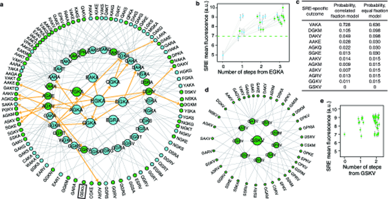
a, Concentric rings contain RH genotypes of minimum path length 1, 2, or 3 steps from AncSR1+11P:EGKA (center). The historical outcome (GSKV, boxed, bottom) is accessible through a three-step path (EGKA – GGKA – GGKV – GSKV). Alternative SRE-specific outcomes accessible in three or fewer steps are in green. Lines connect genotypes separated by a single nonsynonymous nucleotide mutation; lines among genotypes in the outer ring are not shown for clarity. Orange arrows indicate paths of significantly increasing SRE mean fluorescence. b, For trajectories indicated by orange arrows in (a), SRE mean fluorescence is shown versus mutational distance from AncSR1+11P:EGKA (with x-axis jitter to avoid overplotting). Gray lines connect variants separated by single-nucleotide mutations. Error bars, 90% confidence intervals. Green dashed line, activity of AncSR1+11P:GSKV on SRE. c, For the SRE-specific outcomes accessed in orange paths in (a), the probability of each outcome under models where the probability of taking a step depends on the relative increase in SRE mean fluorescence (correlated fixation model), or where any SRE-enhancing step is equally likely (equal fixation model)⁸. d, The historical outcome (GSKV) has SRE-specific single-mutant neighbors. Concentric rings contain SRE-specific RH genotypes of path length 1 or 2 steps from AncSR1+11P:GSKV (center). Lines connect genotypes separated by a single nonsynonymous nucleotide mutation; lines among genotypes in the outer ring are not shown for clarity. e, The distribution of SRE mean fluorescence of SRE-specific neighbors of AncSR1+11P:GSKV illustrated in (d). Error bars, 90% confidence intervals.

Extended Data Figure 6 |. Evolvability of SRE specificity in an ancestral sequence space.

a, Alternative ERE-specific starting points reach SRE-specific outcomes with very different amino acid states. For each starting point accessing ≥15 outcomes (the median of all starting points), the frequency profile of amino acid states at each RH site was determined for the set of SRE-specific outcomes reached in ≤ 3 steps; for each pair of starting points, the Jensen-Shannon distance between profiles was calculated. Blue curve, distribution of pairs of starting points by Jensen-Shannon distances of the outcomes they reach; grey, distribution of Jensen-Shannon distances between profiles for randomly sampled sets of SRE-specific variants. In each modal peak, the amino acid frequency profiles for outcomes reached by a representative pair of ERE-specific starting points are shown. b-d, Contingency in the accessibility of individual SRE-specific outcomes remains when path lengths longer than the historical trajectory are considered. Plots are equivalent to Figs. 2b-d but for trajectories of increasing length.

Extended Data Figure 7 |. The historical starting point cannot access the derived function without permissive mutations.

a, AncSR1 RH functional network layout as in Fig. 3c, with the shortest paths from AncSR1:EGKA to SRE specificity highlighted. The ancestral RH (EGKA) can access SRE specificity. However, all trajectories are at least 5 steps long, require permissive RH changes that confer no SRE activity (e.g. K28R and G26A) and proceed through promiscuous intermediates. b, For paths highlighted in (a), SRE mean fluorescence is shown versus mutational distance from AncSR1:EGKA; gray lines connect variants separated by single-nucleotide mutations. Error bars, 90% confidence intervals. Green dashed line, activity of AncSR1+11P:GSKV on SRE. AncSR1:EGKA was represented by only 7 cells in the SRE library, so its FACS-seq SRE mean fluorescence estimate is unreliable (and its classification was thus inferred by the predictive model). In isolated flow cytometry experiments, its SRE mean fluorescence was indistinguishable from null alleles; the decrease in SRE mean fluorescence from step 0 to step 1 suggested by this figure is therefore more likely a flat line (no change in SRE activity). c, Stochasticity and contingency in trajectories of functional change. Diagrams illustrate paths from a purple starting point (left) to possible green outcomes (right). In a deterministic trajectory (i), a particular genotype encoding the green function will evolve deterministically if selection favors acquisition of the green function and only that genotype is accessible. The outcome of evolution is stochastic (ii) if multiple outcomes are accessible, so which one occurs is random. An outcome is contingent (iii) if its accessibility depends on the prior occurrence of some step that cannot be driven by selection for that outcome. Contingency and stochasticity can occur independently (ii and iii), or they can co-occur in serial (iv).

Extended Data Figure 8 |. The effect of historical permissive substitutions is mediated by nonspecific increases in affinity.

a-d, 11P nonspecifically increase transcriptional activity as measured by FACS-seq, consistent with FoldX predictions of effects on binding affinity. a, Classification of SRE-specific variants as 11P-dependent (orange) and 11P-independent (yellow) based on their functions in AncSR1 and AncSR1+11P backgrounds. Icons for individual variants specifically assessed in (b) and (c) are shown. b, FACS-seq mean fluorescence estimates for 11P-dependent (orange) and 11P-independent (yellow) RH variants in the AncSR1 (left) and AncSR1+11P (right) backgrounds, shown as box-and-whisker plots as in Fig. 4a. Icons represent variants validated in (c). P-values, Wilcoxon rank sum test with continuity correction. The mean fluorescence of 11P-independent genotypes is significantly higher in the AncSR1 background but not in AncSR+11P. c, Validation of apparently restrictive effect of 11P on some genotypes. For three variants nonfunctional in AncSR1+11P but SRE-specific in AncSR1 FACS-seq assays (×), we measured mean fluorescence of isogenic cultures by flow cytometry. We also assayed variants that are SRE-specific in AncSR1+11P and SRE-specific (square) or nonfunctional (open circle) in AncSR1, as validation controls. Isogenic mean fluorescence is represented as mean ± SEM from three replicate transformations and inductions analyzed via flow cytometry. All FACS-seq classifications were validated except for the three apparently restricted variants in AncSR1+11P (highlighted in red), which are in fact strong SRE-activators in this background. Each of these variants was predicted to be a strong SRE-binder based on its genotype, but had an artificially low FACS-seq mean fluorescence estimate, perhaps due to a strong growth defect in inducing conditions. d, After removing the three genotypes with inaccurate FACS-seq fluorescence measurements (×), 11P-independent genotypes have significantly higher mean fluorescence than 11P-dependent genotypes in the AncSR1+11P background, consistent with a nonspecific permissive mechanism via affinity. P-values, Wilcoxon rank sum test with continuity correction. e, 11P do not alter the genetic determinants of SRE specificity. Each plot shows, for a variable site in the library, the frequency of every amino acid state in two functionally defined sets of variants. Spearman’s rho for each correlation is shown. The top row shows that the determinants of SRE specificity are similar in AncSR1 and AncSR1+11P libraries; bottom row shows a much weaker relationship between the determinants of SRE and ERE specificity within the AncSR1+11P library. f, Biochemical determinants of ERE and SRE specificity in the AncSR1 (top) and AncSR1+11P (bottom) backgrounds. A multiple logistic regression model predicts the probability that a variant is RE-specific from the biochemical properties of its amino acid state at each of the four variable RH sites. The coefficients of this model represent the change in log-odds of being ERE-specific or SRE-specific per unit change in each property. Asterisks indicate site-specific determinants that differ significantly between ERE and SRE specificity in each background (Z-test, P < 0.05).

Extended Data Table 1 |. Library sampling statistics.

Sample sizes and sequence read/coverage statistics are shown at various stages of the experimental pipeline for each protein library, yeast reporter strain, and replicate. For details, see Methods.

					FACS					sequencing					coverage, all variants		coverage, coding variants
		bacterial transfor mation yield (cfu)	yeast transfor mation yield (cfu)	smallest bottleneck during FACS induction (cfu)	bin 1 count (cfu)	bin 2 count (cfu)	bin 3 count (cfu)	bin 4 count (cfu)	total number cells recovered post-sort (cfu)	bin 1 read count	bin 2 read count	bin 3 read count	bin 4 read count	read:cfu > 1 for all bins?	median number of cells sampled	fraction variants with >15 cells	median number of cells sampled	fraction variants with >15 cells
AncSRI +11P +RH lib	ERE, rep1	2.32e7	6.12e6	3.2e8	2.02e7	3.38e7	3.22e6	4.74e5	5.77e7	2.75e7	3.64e7	3.32e6	2.01e7	yes	55.4	0.780	61.1	0.797
	ERE, rep 2		1.07 el	4.4e8	1.69e7	1.59e7	2.89e6	1.08e5	3.58e7	3.51 e7	3.65e7	7.91 e6	1.71e6	yes	64.0	0.830	70.5	0.843
	ERE, pooled		1.68e7	Not applicable					9.35e7	Not applicable					127.07	0.913	140.3	0.921
	SRE, rep 1		7.10e6	1.0e8	1.58e7	1.31e7	1.79e6	1.86e5	3.09e7	3.02e7	1.57e7	2.58e6	1.13e6	yes	70.7	0.811	78.2	0.826
	SRE, rep 2		1,83e7	2.0e8	2.02e7	3.17e7	4.91 e6	4.11e5	5.72e7	2.31 e7	6.03e7	1.12e7	3.80e6	yes	64.7	0.836	71.9	0.851
	SRE, pooled		2.54e7	Not applicable					8.81 e7	Not applicable					143.6	0.924	158.9	0.931
AncSRI +RH lib	ERE, rep1	2.26e7	8.31 e6	3.4e8	2.04e7	3.18e7	5.25e6	2.19e5	5.77e7	2.40e7	5.11e7	6.44e6	5.47e5	yes	57.5	0.812	61.3	0.822
	ERE, rep 2		8.63e6	2.6e8	1.58e7	1.61e7	2.82e6	1.56e5	3.49e7	2.50e7	2.85e7	3.54e6	1.12e6	yes	37.1	0.734	39.6	0.748
	ERE, pooled		1,69e7	Not applicable					9.26e7	Not applicable					104.5	0.907	111.7	0.912
	SRE, rep 1		2.04e7	2.5e8	2.10e7	3.57e7	5.40e6	1.33e5	6.22e7	3.26e7	9.27e7	6.57e6	4.32e5	yes	178.4	0.958	191.3	0.961
	SRE, rep 2		2.06e7	2.9e8	2.03e7	3.07e7	5.54e6	5.86e5	5.71 e7	3.14e7	5.53e7	2.01 e7	1.55e6	yes	82.7	0.873	89.1	0.881
	SRE, pooled		4.10e7	Not applicable					1.19e8	Not applicable					289.8	0.979	312.1	0.980

Extended Data Table 2 |. Robustness of inferences to scheme for classification of variants.

Each row represents an inference reported in Figs. 2 and 3; each column is a scheme for functionally classifying variants from FACS-seq data and FACS-seq-trained predictive models. For details of schemes, see Methods.

	Classification Scheme
Inference	Main text	(A) Use FACS-seq ML estimate for AncSRI/ERE	(B) Increase equivalence margin from 20% to 50%	(C) Classify as functional if weak or strong activity	(D) Classify as functional if ML fluorescence >0.8× that of ancestral reference	(E) Classify as functional only if ML fluor within 20% on either side of ancestral reference	(F) Classify all variants based on predictions from genotype	(G) No predictions; classify undetermined variants as inactive	(H) Classify based on prediction or experiment, whichever assigns stronger function	(I) Keep only classifications identical between replicates	(J) Use per- variant estimate of standard error to classify
# ERE-specific, AncSRI	43	138	108	444	67	36	27	39	47	11	47
# promiscuous, AncSRI	45	94	84	158	58	38	45	44	60	30	46
# SRE-specific, AncSRI	41	41	58	213	45	19	31	38	40	39	40
# ERE-specific, AncSRI +11P	144	326	264	619	212	114	101	108	133	76	123
# promiscuous, AncSRI+11P	378	525	554	719	464	254	319	341	459	282	358
# SRE-specific, AncSRI +11P	829	832	1206	2728	956	296	670	768	899	809	837
AncSRI :EGKA requires permissives to access SRE-specificity?	TRUE	TRUE	TRUE	TRUE	TRUE	TRUE	TRUE	TRUE	TRUE	TRUE	TRUE
Shortest patd lengtd from EGKA to SRE- specificity in AncSRI	5	5	3	2	5	6	5	5	5	no paths	4
# SRE-specific outcomes accessed in 3 steps from AncSRI +11P:EGKA	65	66	89	136	77	10	58	53	72	71	65
Proportion ERE-specific starting points unable to access SRE-specificity in 3 steps, AncSR1+11P	0.063	0.037	0.008	0.066	0.014	0.252	0.050	0.139	0.053	0.026	0.089
Proportion SRE-specific outcomes not accessed from any ERE-specific starting point in 3 steps, AncSR1+11P	0.276	0.108	0.118	0.071	0.150	0.571	0.378	0.388	0.276	0.425	0.280
Proportion pairs of ERE-specific starting points witd no shared outcomes in 3 steps, AncSRI+11P	0.542	0.530	0.426	0.229	0.501	0.836	0.543	0.611	0.529	0.390	0.541
Fraction ERE-specific variants witd no patd to SRE-specificity, AncSRI	0.279	0.058	0.505	0.054	0.176	0.378	0.321	0.350	0.250	0.083	0.104
Fraction ERE-specific variants witd no patd to SRE-specificity, AncSRI +11P	0.014	0.021	0.004	0.066	0.005	0.470	0.010	0.056	0.015	0	0.033
Average shortest patd lengtd to SRE- specificity from all connected ERE-specific variants, AncSRI	4.193	4.191	3.796	2.309	4.054	4.304	4.158	4.889	4.278	4.545	4.163
Average shortest patd lengtd to SRE- specificity from all connected ERE-specific variants, AncSRI +11P	2.183	2.122	1.867	1.336	1.986	2.885	2.270	2.333	2.206	2.158	2.294
Fraction ERE-specific variants witd permissive shortest patd, AncSRI	0	0.035	0.059	0.242	0	0	0	0	0	0	0
Fraction ERE-specific variants witd permissive shortest patd, AncSRI +11P	0.290	0.218	0.225	0.191	0.235	0.136	0.207	0.234	0.210	0.140	0.214
Fraction ERE-specific variants witd promiscuous shortest patd, AncSRI	0.483	0.461	0.381	0.370	0.381	0.445	0.548	0.361	0.594	0.634	0.524
Fraction ERE-specific variants witd promiscuous shortest patd, AncSRI+11P	0.413	0.462	0.403	0.133	0.441	0.458	0.504	0.426	0.538	0.524	0.475
Fraction ERE-specific variants witd permissive and promiscuous shortest patd, AncSRI	0.517	0.481	0.530	0.191	0.619	0.555	0.452	0.639	0.406	0.366	0.476
Fraction ERE-specific variants witd permissive and promiscuous shortest patd, AncSRI +11P	0.108	0.120	0.065	0.002	0.082	0.241	0.149	0.164	0.106	0.165	0.135
Fraction ERE-specific variants witd direct shortest path AncSRI	0	0.023	0.030	0.198	0	0	0	0	0	0	0
Fraction ERE-specific variants direct shortest path, AncSRI+11P	0.190	0.201	0.308	0.673	0.242	0.165	0.14	0.176	0.145	0.171	0.176

References

- 1.<Monod J . Chance and Necessity: An Essay on the Natural Philosophy of Biology. (Vintage Books, 1972). [Google Scholar]
- 2.Maynard Smith J Natural selection and the concept of a protein space. Nature 225, 563–564 (1970). [DOI] [PubMed] [Google Scholar]
- 3.Wagner A Neutralism and selectionism: a network-based reconciliation. Nat Rev Genet 9, 965–974 (2008). [DOI] [PubMed] [Google Scholar]
- 4.Hochberg GKA & Thornton JW Reconstructing Ancient Proteins to Understand the Causes of Structure and Function. Annu Rev Biophys 46, 247–269 (2017). [DOI] [PMC free article] [PubMed] [Google Scholar]
- 5.Fowler DM et al. High-resolution mapping of protein sequence-function relationships. Nat Methods 7, 741–746 (2010). [DOI] [PMC free article] [PubMed] [Google Scholar]
- 6.Hietpas RT, Jensen JD & Bolon DNA Experimental illumination of a fitness landscape. P Natl Acad Sci USA 108, 7896–7901 (2011). [DOI] [PMC free article] [PubMed] [Google Scholar]
- 7.Podgornaia AI & Laub MT Pervasive degeneracy and epistasis in a protein-protein interface. Science 347, 673–677 (2015). [DOI] [PubMed] [Google Scholar]
- 8.Wu NC, Dai L, Olson CA, Lloyd-Smith JO & Sun R Adaptation in protein fitness landscapes is facilitated by indirect paths. eLife 5, e16965 (2016). [DOI] [PMC free article] [PubMed] [Google Scholar]
- 9.Aakre CD et al. Evolving new protein-protein interaction specificity through promiscuous intermediates. Cell 163, 594–606 (2015). [DOI] [PMC free article] [PubMed] [Google Scholar]
- 10.Sarkisyan KS et al. Local fitness landscape of the green fluorescent protein. Nature 533, 397–401 (2016). [DOI] [PMC free article] [PubMed] [Google Scholar]
- 11.McKeown AN et al. Evolution of DNA specificity in a transcription factor family produced a new gene regulatory module. Cell 159, 58–68 (2014). [DOI] [PMC free article] [PubMed] [Google Scholar]
- 12.Anderson DW, McKeown AN & Thornton JW Intermolecular epistasis shaped the function and evolution of an ancient transcription factor and its DNA binding sites. eLife 4, e07864 (2015). [DOI] [PMC free article] [PubMed] [Google Scholar]
- 13.Carroll JS et al. Genome-wide analysis of estrogen receptor binding sites. Nat Genet 38, 1289–1297 (2006). [DOI] [PubMed] [Google Scholar]
- 14.Watson LC et al. The glucocorticoid receptor dimer interface allosterically transmits sequence-specific DNA signals. Nat Struct Mol Biol 20, 876–883 (2013). [DOI] [PMC free article] [PubMed] [Google Scholar]
- 15.Luisi BF et al. Crystallographic analysis of the interaction of the glucocorticoid receptor with DNA. Nature 352, 497–505 (1991). [DOI] [PubMed] [Google Scholar]
- 16.Schwabe JW, Chapman L, Finch JT & Rhodes D The crystal structure of the estrogen receptor DNA-binding domain bound to DNA: how receptors discriminate between their response elements. Cell 75, 567–578 (1993). [DOI] [PubMed] [Google Scholar]
- 17.Zilliacus J, Carlstedt-Duke J, Gustafsson JA & Wright AP Evolution of distinct DNA-binding specificities within the nuclear receptor family of transcription factors. P Natl Acad Sci USA 91, 4175–4179 (1994). [DOI] [PMC free article] [PubMed] [Google Scholar]
- 18.Bain DL et al. Glucocorticoid receptor-DNA interactions: binding energetics are the primary determinant of sequence-specific transcriptional activity. J Mol Biol 422, 18–32 (2012). [DOI] [PubMed] [Google Scholar]
- 19.Eick GN, Bridgham JT, Anderson DP, Harms MJ & Thornton JW Robustness of Reconstructed Ancestral Protein Functions to Statistical Uncertainty. Mol Biol Evol 34, 247–261 (2017). [DOI] [PMC free article] [PubMed] [Google Scholar]
- 20.Bloom JD, Gong LI & Baltimore D Permissive secondary mutations enable the evolution of influenza oseltamivir resistance. Science 328, 1272–1275 (2010). [DOI] [PMC free article] [PubMed] [Google Scholar]
- 21.Gong LI, Suchard MA & Bloom JD Stability-mediated epistasis constrains the evolution of an influenza protein. eLife 2, e00631 (2013). [DOI] [PMC free article] [PubMed] [Google Scholar]
- 22.Harms MJ & Thornton JW Evolutionary biochemistry: revealing the historical and physical causes of protein properties. Nat Rev Genet 14, 559–571 (2013). [DOI] [PMC free article] [PubMed] [Google Scholar]
- 23.Starr TN & Thornton JW Epistasis in protein evolution. Protein Sci 25, 1204–1218 (2016). [DOI] [PMC free article] [PubMed] [Google Scholar]
- 24.Dickinson BC, Leconte AM, Allen B, Esvelt KM & Liu DR Experimental interrogation of the path dependence and stochasticity of protein evolution using phage-assisted continuous evolution. P Natl Acad Sci USA 110, 9007–9012 (2013). [DOI] [PMC free article] [PubMed] [Google Scholar]
- 25.Ortlund EA, Bridgham JT, Redinbo MR & Thornton JW Crystal structure of an ancient protein: evolution by conformational epistasis. Science 317, 1544–1548 (2007). [DOI] [PMC free article] [PubMed] [Google Scholar]
- 26.Harms MJ & Thornton JW Historical contingency and its biophysical basis in glucocorticoid receptor evolution. Nature 512, 203–207 (2014). [DOI] [PMC free article] [PubMed] [Google Scholar]
- 27.Natarajan C et al. Predictable convergence in hemoglobin function has unpredictable molecular underpinnings. Science 354, 336–339 (2016). [DOI] [PMC free article] [PubMed] [Google Scholar]
- 28.Shah P, McCandlish DM & Plotkin JB Contingency and entrenchment in protein evolution under purifying selection. P Natl Acad Sci USA 112, E3226–E3235 (2015). [DOI] [PMC free article] [PubMed] [Google Scholar]
- 29.Bridgham JT, Ortlund EA & Thornton JW An epistatic ratchet constrains the direction of glucocorticoid receptor evolution. Nature 461, 515–519 (2009). [DOI] [PMC free article] [PubMed] [Google Scholar]
- 30.Lynch M & Hagner K Evolutionary meandering of intermolecular interactions along the drift barrier. P Natl Acad Sci USA 112, E30–E38 (2015). [DOI] [PMC free article] [PubMed] [Google Scholar]
- 31.Fox JE, Bridgham JT, Bovee TFH & Thornton JW An evolvable oestrogen receptor activity sensor: development of a modular system for integrating multiple genes into the yeast genome. Yeast 24, 379–390 (2007). [DOI] [PubMed] [Google Scholar]
- 32.Mumberg D, Müller R & Funk M Yeast vectors for the controlled expression of heterologous proteins in different genetic backgrounds. Gene 156, 119–122 (1995). [DOI] [PubMed] [Google Scholar]
- 33.Gietz RD & Woods RA Transformation of yeast by lithium acetate/single-stranded carrier DNA/polyethylene glycol method. Methods Enzymol 350, 87–96 (2002). [DOI] [PubMed] [Google Scholar]
- 34.<R Core Team. R: A language and environment for statistical computing. R Foundation for Statistical Computing, Vienna, Austria: URL https://www.R-project.org/ (2016). [Google Scholar]
- 35.Muggeo V Segmented: an R package to fit regression models with broken-line relationships. R news; (2008). [Google Scholar]
- 36.Sluder AE, Mathews SW, Hough D, Yin VP & Maina CV The nuclear receptor superfamily has undergone extensive proliferation and diversification in nematodes. Genome Res 9, 103–120 (1999). [PubMed] [Google Scholar]
- 37.Benatuil L, Perez JM, Belk J & Hsieh CM An improved yeast transformation method for the generation of very large human antibody libraries. Protein Eng Des Sel 23, 155–159 (2010). [DOI] [PubMed] [Google Scholar]
- 38.Scanlon TC, Gray EC & Griswold KE Quantifying and resolving multiple vector transformants in S. cerevisiae plasmid libraries. BMC Biotechnol 9, 95 (2009). [DOI] [PMC free article] [PubMed] [Google Scholar]
- 39.Fowler DM, Stephany JJ & Fields S Measuring the activity of protein variants on a large scale using deep mutational scanning. Nat Protoc 9, 2267–2284 (2014). [DOI] [PMC free article] [PubMed] [Google Scholar]
- 40.Mir K, Neuhaus K, Bossert M & Schober S Short Barcodes for Next Generation Sequencing. PLOS ONE (2013). doi: 10.1371/journal.pone.0082933.g001 [DOI] [PMC free article] [PubMed] [Google Scholar]
- 41.Peterman N & Levine E Sort-seq under the hood: implications of design choices on large-scale characterization of sequence-function relations. BMC Genomics 17, 206 (2016). [DOI] [PMC free article] [PubMed] [Google Scholar]
- 42.Delignette-Muller ML & Dutang C fitdistrplus: An R package for fitting distributions. J Stat Softw 64 (2015). [Google Scholar]
- 43.Archer KJ & Williams AAA L1 penalized continuation ratio models for ordinal response prediction using high-dimensional datasets. Stat Med 31, 1464–1474 (2012). [DOI] [PMC free article] [PubMed] [Google Scholar]
- 44.<Vega Yon J, J Fábrega Lacoa & Kunst JB. rgexf: Build, Import and Export GEXF Graph Files. R package version 0.15.3. https://CRAN.R-project.org/package=rgexf (2015).
- 45.Bastian M, Heymann S & Jacomy M Gephi: an open source software for exploring and manipulating networks. ICWSM; (2009). [Google Scholar]
- 46.Csardi G & Nepusz T The igraph software package for complex network research. Complex Systems; 1695 (2006). [Google Scholar]
- 47.Sailer ZR & Harms MJ Detecting high-order epistasis in nonlinear genotype-phenotype maps. Genetics 205, 1079–1088 (2017). [DOI] [PMC free article] [PubMed] [Google Scholar]
- 48.Knol MJ, Pestman WR & Grobbee DE The (mis)use of overlap of confidence intervals to assess effect modification. Eur J Epidemiol 26, 253–254 (2011). [DOI] [PMC free article] [PubMed] [Google Scholar]
- 49.Schymkowitz J et al. The FoldX web server: an online force field. Nucleic Acids Res 33, W382–W388 (2005). [DOI] [PMC free article] [PubMed] [Google Scholar]
- 50.Luscombe NM, Laskowski RA & Thornton JM NUCPLOT: a program to generate schematic diagrams of protein-nucleic acid interactions. Nucleic Acids Res 25, 4940–4945 (1997). [DOI] [PMC free article] [PubMed] [Google Scholar]
- 51.Schymkowitz JWH et al. Prediction of water and metal binding sites and their affinities by using the Fold-X force field. P Natl Acad Sci USA 102, 10147–10152 (2005). [DOI] [PMC free article] [PubMed] [Google Scholar]
- 52.Crooks GE, Hon G, Chandonia J-M & Brenner SE WebLogo: a sequence logo generator. Genome Res 14, 1188–1190 (2004). [DOI] [PMC free article] [PubMed] [Google Scholar]
- 53.Abriata LA, Palzkill T & Dal Peraro M How structural and physicochemical determinants shape sequence constraints in a functional enzyme. PLOS ONE 10, e0118684 (2015). [DOI] [PMC free article] [PubMed] [Google Scholar]
- 54.Paternoster R, Brame R, Mazerolle P, & Piquero A Using the correct statistical test for the equality of regression coefficients. Criminology 36, 859–866 (1998). [Google Scholar]
Associated Data
This section collects any data citations, data availability statements, or supplementary materials included in this article.
Supplementary Materials
Data Availability Statement