Pulmonary Artery-Vein Classification in CT Images Using Deep Learning

Abstract

Recent studies show that pulmonary vascular diseases may specifically affect arteries or veins through different physiologic mechanisms. To detect changes in the two vascular trees, physicians manually analyze the chest computed tomography (CT) image of the patients in search of abnormalities. This process is time-consuming, difficult to standardize and thus not feasible for large clinical studies or useful in real-world clinical decision making. Therefore, automatic separation of arteries and veins in CT images is becoming of great interest, as it may help physicians accurately diagnose pathological conditions.

In this work, we present a novel, fully automatic approach to classifying vessels from chest CT images into arteries and veins. The algorithm follows three main steps: first, a scale-space particles segmentation to isolate vessels; then a 3D convolutional neural network (CNN) to obtain a first classification of vessels; finally, graph-cuts (GC) optimization to refine the results.

To justify the usage of the proposed CNN architecture, we compared different 2D and 3D CNNs that may use local information from bronchus- and vessel-enhanced images provided to the network with different strategies. We also compared the proposed CNN approach with a Random Forests (RF) classifier.

The methodology was trained and evaluated on the superior and inferior lobes of the right lung of eighteen clinical cases with non-contrast chest CT scans, in comparison with manual classification. The proposed algorithm achieves an overall accuracy of 94%, which is higher than the accuracy obtained using other CNN architectures and RF. Our method was also validated with contrast-enhanced CT scans of patients with Chronic Thromboembolic Pulmonary Hypertension (CTEPH) to demonstrate that our model generalizes well to contrast-enhanced modalities.

The proposed method outperforms state-of-the-art methods, paving the way for future use of 3D CNN for A/V classification in CT images.

I. Introduction

In the last decades, computed tomography (CT) has become the most common imaging modality for diagnosis and assessment of lung disease [1], [2]. Modern CT scanners combined with modern imaging techniques allow for the use of low radiation doses to (semi-)automatically identify and extract pulmonary structures, such as vessels and bronchi with relatively high accuracy. However, despite the recent progress in segmentation techniques for CT images, many tasks remain unresolved. Among them, recognition and discrimination of pulmonary arteries and veins represent one of the most challenging problems.

Classification of lung vessels into artery/vein (A/V) may be of great help for physicians to accurately diagnose pulmonary diseases that may affect either the arterial or the venous trees in specific ways. As an example, recent studies show that A/V classification allows for better assessment of pulmonary emboli [3], whereas changes in the arterial tree have been associated with the development of chronic thromboembolic pulmonary hypertension (CTEPH) [4]. Also, changes in intraparenchymal pulmonary arteries have been associated with evidence of right ventricular dysfunction [5], [6].

A basic approach to separate the two vascular trees consists in the manual inspection of individual CT slices to trace the vessels back to their origin in search of features that specifically characterize arteries and veins. However, intrinsic issues of CT images, like a large number of slices, scan resolution, and partial volume effect, along with the extreme complexity and density of the vessel tree, make this manual separation a long and tedious job, which may be prone to mistakes. For this reason, having a method to (semi-)automatically segment vascular structures on CT images may be crucial to improve the physician’s ability to assess pathological conditions.

Throughout the years, several methods have been proposed to either enhance or segment vessels from lung CT images [7]. Although these methods are not able to separate arteries and veins, they are often used as a starting point for most of the A/V segmentation algorithms available in the literature [8]–[12]. Moreover, most methods try to utilize A/V local information, like seed points automatically defined in the lung region [13], [14] or the proximity of arteries to bronchi [12], to separate the two vascular trees.

The idea of exploiting the proximity of airways to arteries to classify vessels was used in several other methods available in the literature. In [8] a method which searched for airways in the neighborhood of vessel segments (defined as the portion of a vessel between two branching points) to define an arterialness measure was proposed. The arterialness is assigned a higher value when the vessel segment and the near bronchus run parallel to each other. However, the risk of mislabeling vessels using this method increases with decreasing vessel radius, as on CT images small vessels are better visible than bronchi of similar size. In [9], A/V separation is performed integrating the assumption of proximity of arteries and bronchi with the idea that veins run close to the inter-lobar fissures (estimated by a Voronoi diagram). However, this work lacks a method for accurate extraction of vessel regions and a proper comparison set, as it has been tested only on 3 CT images. [10], [11] designed an algorithm that utilizes a morphological multiscale opening operator with differently sized kernels to separate attached arteries and veins at various scales and locations, starting from two sets of manually picked seed points. Although a specific GUI was introduced in [11] to pick the points, this manual operation requires high expertise and may be tedious. The method in [14] consists in the construction of a minimum-spanning-tree and an edge cutting step to separate vessel branches. The main drawback of this method is represented by the final crucial step that involves manual interaction to refine the A/V separation. In [15], a novel fully-automatic algorithm is proposed. This method exploits the energy minimization of higher-order potentials, where the higher-order cliques are chosen according to the data and on the prior knowledge about the desired shape, to encourage sets of voxels to belong to arteries or veins entirely. The method was evaluated on ten chest CT Angiography images, considering only vessels with CT values more than 200 HU in the lungs.

Recently, two works have been published with the aim of improving available A/V segmentation approaches [12], [16]. In [16], the vessel tree is represented as a graph and local information is used to extract a set of small sub-trees. The sub-trees are linked to each other by analyzing the peripheral vessels under the assumption that since arteries and veins only meet at alveolar sacks, which are far below the CT resolution, they merely approach each other in the vessel segmentation. Classification is then done by simply considering the difference in the vessel sub-tree volumes. Although this method does not need information about airways, discrimination based only on the volume of the trees may not be ideal, especially in patients with specific diseases that may differentially affect arterial and venous volumes, or that may have different effects on different regions of the lung. In [12], a fully automatic A/V separation algorithm based on [8] is proposed. Vessels are classified by combining both local and global properties using two integer programs. First, vessel sub-trees are extracted based on vessel geometry. Then, a second integer program is performed to use two anatomical properties of the vessels: the uniform distribution of arteries and veins, computed using a Voronoi diagram, and the close proximity of arteries and bronchi, measured by means of a specific arterialness measure. The method was tested on 25 non-contrast CT images and is reported to outperform [14]. However, the method is highly sensitive to parameters, with those used for calculation of arterialness being the most effective.

In this work, we present a fully automatic algorithm that combines a convolutional neural network (CNN) approach [17] with a graph-cuts (GC) strategy [18], [19] to classify vessels into arteries and veins on chest CT images. Small 3D patches are extracted from the CT image around the vessel candidates, defined using the scale-space particles approach described in [20], [21], and used to train the neural network.

A preliminary version of this paper was proposed in [22]. In the present paper, a new CNN architecture that uses 3D convolutions is proposed and compared to five alternative architectures that are provided different patches as input. The goal is to demonstrate that 3D convolutions are more effective in separating arteries from veins than 2D convolutions, where only workarounds can be used to provide connectivity information to the network. To prove this hypothesis, a full evaluation and analysis of results are performed. Moreover, the proposed method is compared to the method in [16], and the ability of the algorithm to perform AV segmentation both on non-contrast and contrast CT images and to generalize results to whole lungs, despite being trained on only two lobes, is demonstrated.

To justify the use of the proposed CNN architecture, we compared different CNN strategies for both 2.5D and 3D patches. First, we followed the idea proposed in [12] to exploit the proximity of bronchi to arteries and combined the original CT patches with bronchus-enhanced patches and vessel-enhanced images. Then, for a better comparison between 2D and 3D approaches, 2.5D patches were constructed taking into account connectivity information of the single particles, based on their location and strength.

Eighteen non-contrast thoracic CT scans from the COPDGene study [23] were used to perform a quantitative evaluation by assessing agreement between human observers and the proposed method. Comparison between CNN and Random Forests (RF) [24], a different machine learning approach, was also performed. To get a proper comparison with competing methods, we also evaluated the proposed method on the annotated CT images provided by [16].

We then set up two tests in an attempt to explain the obtained results. First, an analysis of the results sub-divided into three groups based on vessel size (defined by the particles scale) was performed to assess the sensitivity of A/V classification to vessel size. Then, we computed the receiver operating characteristic (ROC) curve to evaluate sensitivity and specificity of the different machine learning classifications.

Finally, to further validate the algorithm and demonstrate its reliability across different cohorts and modalities, we tested the proposed method on a group of 33 contrast CT images from patients with and without chronic thromboembolic pulmonary hypertension (CTEPH) using the model trained with non-contrast CT cases.

II. Methods

The outline of the proposed method is shown in Fig. 1. Our A/V classification follows three main steps. First, we extract the lung region from the chest CT image and segment vessels using a scale-space particles algorithm to define vessel candidates (Section II-A). Then, we train a CNN architecture using 3D patches extracted from the CT image around the computed particles. To justify the use of this architecture, we compared it to five different CNNs that use 2D and 3D patches extracted around the CT image with or without additional local information (Sections II-B and II-C).

Fig. 1.

Overview of the proposed method for A/V classification. After lung and vessel segmentation, a 3D CNN algorithm is implemented in combination with GC optimization to classify vessel candidates into arteries and veins.

Since each patch is extracted around a single particle, A/V classification with CNN is carried out independently on each point. This may cause spatial inconsistency in the vessel segments. Therefore, the last step consists in a classification refinement achieved using a graph-cuts optimization [18], [19] that combines both connectivity and pre-classification knowledge to obtain the final A/V segmentation (Section II-D).

A. Pre-processing Operations

The first step of the proposed method consists in extracting the vascular tree from the CT image to define the vessel candidates for A/V classification. To this end, we first segment the lung region using the method described in [25]. Then, a vessel enhancement is applied in the lung area using a Frangi filter [26] with parameters α = 0.53 and β = 0.61 (obtained by implementing a grid search that used a Dice coefficient score to compare the output of the particles algorithm to manual segmentation) followed by a thresholding and a binary skeletonization to define initial candidate locations.

In addition to location, the patch extraction method here implemented also requires vessel orientation. For this reason, the skeletonized vessel mask is used as input to the scale-space particles sampling method described in [20], [21]. This approach starts from a vessel mask and exploits the second-order local information of the image (Hessian matrix) to identify and represent the vascular tree as a collection of particles, a set of points containing information about vessel scale, orientation (through Hessian eigenvectors and eigenvalues), and intensity of the considered vessel. This approach capitalizes on the multi-scale self-similarity of the vasculature, making it more robust to noise in the smaller vessels than typical approaches. An example of lung vessel extraction through scale-space particles is given in Fig. 2. Particles provide a convenient representation of a tree geometry as the particles know the local orientation of the vessel axis based on the corresponding Hessian eigenvector as a by-product of the optimization. Nevertheless, our method is general to other vascular segmentation approaches for which a skeleton can be easily extracted, and the vessel orientation can be resolved by standard scale-space analysis or by means of local connectivity of skeleton points.

Fig. 2.

Example of vessel segmentation from a clinical chest CT image through the scale-space particles method.

B. Proposed Method

Once the vessel candidates are extracted, an initial A/V classification is performed for each particle using CNN. We compared the proposed CNN with five different architectures, based on the patch dimensionality (2- or 3-D) and whether vessel strength and arterialness are considered.

In the following sections, we first describe the proposed approach, both regarding patch extraction and CNN architecture, and then we detail the alternative architectures used for comparison.

1) Patch Extraction

The proposed CNN utilizes only 3D patches extracted from the CT image around the vessel of interest. A central patch covering a neighborhood of 32×32 pixels is extracted on the reformatted plane along the particle’s main axis, given by the first eigenvector of the Hessian matrix and obtained using an isotropic spacing of 0.625 mm, achieved by resampling the original image by means of cubic interpolation. The 3D patch is then obtained considering the patch of the given central particle and the patches around 4 particles (two above and two below) belonging to the same vessel along its reformatted direction. Therefore, every patch represents a small vessel segment of 32×32×5 voxels on the reformatted plane along the vessel of the considered point.

2) CNN Architecture

Fig. 3 shows the architecture of the proposed CNN. The network consists of three convolutional layers separated by a single max pooling and two dropout layers and followed by three fully-connected layers.

Fig. 3.

The proposed 3D CNN classifier for A/V segmentation. 3D patches are extracted from the CT image around vessel candidates defined by a scale-space particle algorithm. The CNN learns A/V characteristics on these patches through three 3D convolutional layers, one max pooling and three fully connected layers.

C. Alternative CNNs

We hypothesize that a 3D approach performs better than 2D CNNs for AV segmentation, as connectivity information plays a very important role in the distinction of the two trees, which using 2D CNNs can be simulated only by means of specific workarounds. Moreover, we considered that the inclusion of more information, such as the one provided by bronchus- and vessel-enhanced images do not particularly help the network to better learn characteristics of arteries and veins. To demonstrate this hypothesis, we defined five alternative CNN architectures to be compared with the proposed one. To this end, we extracted 2D and 3D patches around each particle point with different strategies. A summary of the data patches provided to the different CNN architectures is described in Table I.

TABLE I.

Summary of the patch sizes for all the different CNNs utilized in this work. Ch. stands for channels, MI for multi-inputs (indicating that CT and enhanced images are used as separate inputs to the network), and # is used for number.

	# Ch.	Enhanced images (Y/N)	# of patches	# patches × (x, y, depth, ch.)
Proposed
3D CT only	1	N	1	1×(32,32,5,1)
Alternatives
1. 2.5D CT only	1	N	1	1×(32,32,1,3)
2. 2.5D 3 Ch.	9	Y	1	1×(32,32,1,9)
3. 2.5D MI	3	Y	3	3×(32,32,1,3)
4. 3D 3 Ch.	3	Y	1	1×(32,32,5,3)
5. 3D MI	1	Y	3	3×(32,32,5,1)

1) Alternative Patch Extraction

For the extraction of 3D patches, we used the same approach used for the proposed method, while for 2D patches we considered only the neighborhood region of 32×32 pixels on the reformatted plane of the particles. However, since connectivity between vessel points may provide crucial information for A/V classification, we also combined the 2D patch of the sample of interest with those of the two closest particles that have the most similar orientation. The difference with a 3D patch is given by the fact that the extracted patches are merged to the original patch as additional channels, in an attempt to simulate a 3D representation and obtain a better comparison. We define these patches as 2.5D. Therefore, a 2.5D patch extracted around a vessel candidate consists of 32×32 pixels and three channels, defined by the CT images of the central point and the two points most proximal to it (2.5D CT only, alternative 1 in Tab. I).

To determine whether CNN may benefit from the inclusion of structural information (such as bronchi-arteries proximity) to separate arteries from veins, in four of the five alternative architectures we included the bronchus- and vessel-enhanced images. While the inclusion of the vessel-enhanced image might be redundant, as the whole analysis is based on particles that come from the vascular structure, we considered that some additional local information of the vessel might be identified and analyzed by the CNN on this image. For the enhancement, we used a Frangi filter [26], with optimal parameters defined by means of grid search (that compared the result of the particles algorithm to manual segmentation using a Dice coefficient score as metric), to enhance vessels and bronchi from CT images (α = 0.53, β = 0.61, and C=245 for vessel enhancement, α = 0.29, β = 0.77, and C=105 for enhancement of airways). From these enhanced images, we then extracted 2D and 3D patches around the candidate points, and we integrated these patches to those of the CT using two different strategies. In the first case, we integrated them as new channels of the patch (2.5D 3 Ch. or 3D 3 Ch., alternatives 2 and 4 in Tab. I). In a second approach, we let the network learn from the three patches independently, and we concatenate them at the fully connected level (2.5D 3 MI or 3D 3 MI, alternatives 3 and 5 in Tab I). As an example, a 2.5D patch with enhanced images integrated as additional channels consists of 32×32 pixels around the particle point and 9 channels, given by the CT, the bronchus-enhanced, and the vessel-enhanced images of the central point and the two most proximal ones. On the other hand, if the enhanced images are used as independent inputs of the 2D network, three patches of 32×32 pixels and three channels (central point and two closest ones) are used.

2) 2D Architecture (Alternative Networks 1 to 3)

Fig. 4 shows the architecture of the CNN when using 2.5D patches with either the only CT image or with the inclusion of enhanced images as additional channels or as separate inputs. As shown, the basic CNN architecture is the same in all three cases. Five 2D convolutional layers separated and followed by two max pooling and two dropout layers, respectively, and three fully-connected layers define the network structure.

Fig. 4.

Scheme of the CNN architectures using 2.5D patches around the vessel particles. The CNN takes as input either patches from only the CT image (blue) or from the CT combined with the enhanced images, integrated either as additional channels or as separate inputs. Patch size is reported as: number of patches × (x,y, channels)

Although the architecture remains the same, when providing arterialness and vessel strength as separate inputs on top of the local information provided by the CT, the convolutions and max-pooling operations are executed in parallel on the three inputs to let the network learn new features from each patch independently. Therefore, the obtained weights and biases are concatenated just before the fully connected operations begin. The hyper parameters of each network have been empirically chosen to optimize results for the specific problem at hand.

3) 3D Architecture (Alternative Networks 4 and 5)

The CNN architectures for the 3D patches when using the enhanced images either as additional channels or as external inputs are presented in Fig. 5. For both cases, the structure is the same as the one used for the proposed CNN, with the only difference that the same operations are run in parallel in case arterialness and vesselness are provided as external patches, and, as for the 2D CNNs, with the hyper parameters empirically chosen to optimize results for each network.

Fig. 5.

Scheme of the two alternative CNN architectures using 3D patches around the vessel particles. The CNN takes as input patches extracted from the CT image and the vessel- and bronchi-enhanced images, integrated either as additional channels (blue) or as separate inputs (red). Patch size is reported as: number of patches × (x,y, depth, channels)

D. Final Graph-Cuts Refinement

Despite efforts to provide enough spatial information to the network to ensure spatial consistency, inconsistencies may still occur during A/V classification (see Fig. 6), mainly due to the presence of touching and intertwined areas in the two vascular trees and because classification is done on each particle independently without explicitly modeling the smoothness at the tree level. For this reason, once the initial classification with CNN is concluded, we employ an automatic graph-cuts (GC) strategy to refine the classification. To this end, we use the approach described in [27], which combines graph theory [28], that aggregates a set of subtrees into a graph, with methods for energy minimization to find the minimum-cuts in the graph that defines the optimal solution. In particular, a graph consists of a set of vertexes 𝒱 = {v_i | i = 1… N_nodes} and a set of edges connecting different nodes ε = {(v_i, v_j) | i, j = 1… N_nodes}. The set of vertexes include two terminal (or virtual) nodes, source, s and sink, t, s. t. 𝒱_t = {s} ∪ {t}, and a group of real non-terminal nodes, 𝒱_n-t. Similarly, ε contains two types of edges; edges connecting pairs of non-terminal nodes (known as n_links), ε_n-t = {(v_i, v_j) | v_i, v_j ∈ 𝒱_n-t}, and edges that connect one terminal node with a non-terminal node (t_links), ε_t = {(s, v_i)∪(vi, t) | v_i ∈ 𝒱_n-t and s, t ∈ 𝒱_t}. The search for the minimum cut is an energy minimization problem, where the energy is defined as:

$$ℰ={ℰ}_{\mathit{bound}}+{ℰ}_{\mathit{reg}}$$ (1)

where 𝔼_bound is the boundary term that designate the coherence between neighborhood nodes (connectivity information) and it is given by the weights of the n_links, while 𝔼_reg represents the regional term that describes the likelihood of each class (artery-vein similarity score), given by the weights of the t_links. Therefore, the minimal cut gives the classification that globally minimizes the combination of both energies.

Fig. 6.

An example of spatial inconsistency obtained after CNN classification.

In the problem proposed here, the artery-vein similarity score of the regional term, represented by the edges ε_t, is provided by the probability obtained in the pre-classification step using CNN. Therefore, the weights of the edges t_links are directly fixed to the probabilistic estimations:

$$w(s,p_i)=P_{\mathit{artery}}(p_i)$$ (2)

$$w(p_i,t)=P_{\mathit{vein}}(p_i)=1-P_{\mathit{artery}}(p_i)$$ (3)

with p_i being the i-th particle and P(p_i) indicating the computed probability.

On the other hand, the boundary term, represented by ε_n-t, should include information about the connectivity of particles. Since particles do not provide this information, and due to the complex topology of arterial and venous trees, a conservative structural connectivity strategy is used, which initially allows the creation of links between each particle and all the particles within a cylinder created along the main direction of the vessel with radius r_neigh = 3mm (empirically tweaked after several tests). To avoid issues in areas with high density of edges, we also empirically fixed the number of possible connections that a node is allowed to have (N_con = 5). In order to define the weight of the n_links, which represents the strength of the connections between particles, three main characteristics are considered. First, scale consistency, (w_σ(p1, p2)): two particles with similar scale have a higher probability of being neighbors. Second, particle proximity w_dist(p1, p2): the closer the particles are in terms of Euclidean distance, the higher the probability of belonging to the same tree. Finally, direction consistency (w_||(p1, p2)): defined by the parallelism between the connectivity vector between two particles and the local direction of the considered particles. Therefore, based on these three characteristics, we can construct different weighting functions to define the strength of the n_links:

$$w(p_1,p_2)=f(w_{\sigma }(p1,p2),w_{\mathit{dist}}(p1,p2),w_{\left|\right|}(p1,p2))$$ (4)

In some cases, the restriction introduced to construct the n_links may create a few isolated sub-trees that may complicate the classification. For this reason, after a first GC classification, a final step is executed to connect all edges of the sub-trees iteratively. In particular, the following steps are repeated until the whole graph consists of a single connected component: a) the biggest connected component is selected as principal one; b) the Euclidean distance between the points belonging to the isolated sub-trees and the principal component is computed; c) the particles belonging to the isolated sub-trees with minimum distance are connected by an edge with weight defined by Eq. (4).

Once the final graph is obtained, the minimum cut, C_min is computed using the min-cut/max-flow conversion proposed in [18], providing a partition of the graph G into two connected components G₁ and G₂:

$$C_{\mathit{min}}=\underset{G_1,G_2}{\text{argmin}}(ℰ(G_1,G_2))=\underset{G_1,G_2}{\text{argmin}}({ℰ}_{\mathit{bound}}(G_1,G_2)+\alpha ·{ℰ}_{\mathit{reg}}(G_1,G_2))$$ (5)

where α = 8 was found as optimal by means of grid search to balance the regional and boundary terms:

$${ℰ}_{\mathit{bound}}(S,T)=\sum _{\begin{array}{l}{p}_1\in S\cap {\mathcal{V}}_{n-t}\\ p_2\in T\cap {\mathcal{V}}_{n-t}\\ (p_1,p_2)\in {\epsilon }_{n-t}\end{array}}w(p_1,p_2)$$ (6)

$${ℰ}_{\mathit{reg}}(S,T))=(\sum _{\begin{array}{c}{p}_1\in S\cap {\mathcal{V}}_{n-t}\\ (p_1,t)\in {\epsilon }_t\end{array}}w(p_1,t)+\sum _{\begin{array}{c}{p}_2\in T\cap {\mathcal{V}}_{n-t}\\ (s,p_2)\in {\epsilon }_t\end{array}}w(s,p_2))$$ (7)

III. Experimental Setup

A. Data Description

We trained and evaluated the proposed method on twenty-one non-contrast CT scans from patients with COPD randomly extracted from the COPDGene study [23]. The scans were acquired using multi-detector CT scanners with at least 16 detector channels. COPDGene centers were approved by their Institutional Review Boards and all subjects provided written informed consent. For the COPDGene study, CT scans are acquired using multi-detector CT scanners (at least 16 detector channels).

For this study, we used only CT images acquired on full inspiration (200 mAs) that have been reconstructed with sub-millimeter slice thickness and a smooth reconstruction kernel, and with voxel size varying from 0.6 to 0.75 mm. More information on the acquisition protocols used for the COPDGene study can be found in [23]. For each subject, only the right lung, which was segmented and separated into its three lobes using the method described in [29], was considered. In this study, only upper and lower lobes were utilized. This gives us a total of 42 independent lobes for AV classification, as the two lobes present specific and unique characteristics.

To create a reference standard for evaluation, manual labeling of arteries and veins was performed by a pulmonary expert for each of the two lobes. To this end, the Kruskal’s minimum spanning tree algorithm [30] was used to connect vessel particles. A relative angle of greater than 20 degrees or a gap of greater than 5mm between adjacent particles served as break points in the tree, creating a set of vessel segments. Segments with 4 or fewer particles were discarded. A 3D rendering of the vasculature superimposed on the initial CT scan allowing for scrolling in all three planes was used to trace the origins of the proximal vessels to the main pulmonary artery and the pulmonary veins. Once proximal segments were labeled, distal segments were then similarly traced back to the proximal segments that were already marked by tracing the vasculature to make sure that the segments were indeed connected. This was repeated until all distal segments were marked [31]. As a final result, a total of 693,287 particles (384,710 arteries, 308,577 veins) have been labeled.

For the training of the convolutional neural networks, we use both lobes of three subjects, corresponding to a total of six lobes that include 56,667 particles for arteries, and 39,914 particles for veins. The remaining 36 lobes from eighteen subjects (596,706 particles with 328,043 arteries and 268,663 veins points) were used for evaluation. Both lobes of two subjects (69,895 particles) were used for validation during training.

We also validated the proposed network trained on non-contrast CT scans on the full lung (considering all lobes) of thirty-three patients with computed tomography pulmonary angiograms (CTPA) retrospectively acquired for presenting potential clinical evidence of CTEPH [6]. 18 subjects were diagnosed with CTEPH by a panel of experts based on their hemodynamics and imaging characteristics, while 15 were assigned to a control group as no evidence of pulmonary or heart disease was found. These subjects all had CT angiograms of the lungs within one year of invasive testing. The reference standard of arteries and veins was created by a pulmonary expert that manually labeled each particle following the same approach used for the COPDGene cohort. A total of 976,417 arteries and 786,674 veins were labeled corresponding to the 33 subjects.

B. Training Details

Before starting the network training, the intensity values of the single patches were standardized by subtracting the patch mean and dividing by the patch’s standard deviation, in an attempt to make A/V classification independent from image characteristics and contrast.

All CNN architectures were trained for a total of 200 epochs using a Nesterov-momentum update using a cross-entropy loss function and with a softmax function as output nonlinearity, which is a typical choice in classification tasks, with a learning rate of 0.01, and batch size of 128. A rectified linear unit (ReLU) was used as activation for both convolutional and fully connected layers, while a Glorot uniform was selected to initialize the weights of the convolutional kernels. Zero-padding was used for the convolutional inputs so that the output has the same length as the original input. Finally, early stopping (with a latency of 30 epochs, monitoring the validation loss with a delta of 0.1) was implemented and data was augmented during training by generating random rotation of the patches to avoid overfitting.

All CNN operations were computed on an NVIDIA Titan X GPU machine, using the deep learning framework Keras [32] on top of TensorFlow [33], [34].

C. Evaluation Experiments

To evaluate the performance of the proposed algorithm, we carried out two main experiments on all cases not used during the training phase. First, we compared the classification obtained using the proposed approach to the reference standard manually created as described in Section III-A. To this end, we computed a per-particle accuracy measure. The accuracy is computed for all CNN architectures for both steps of the algorithm: after CNN, classifying all particles with a probability higher than a 0.5 threshold as arteries and all other points as veins, and after applying GC with the refined graph. Sensitivity and specificity (considering arteries as the positives) of each method were also computed.

As a second experiment, we compared the accuracy obtained with the proposed method and the other CNNs to those obtained using an RF approach [24] as the initial classifier for GC. The RF implementation is described in Section III-D. As for the first experiment, we used accuracy as the main testing measure, and we completed the evaluation with the analysis of sensitivity and specificity of the different methods.

As an additional test, we compared the proposed method to the one proposed in [16], where a dataset of 55 CT scans has been made publicly available. For these datasets, annotations were divided into two separate sets. The first set consists of full annotation of all vessel in a subset of ten randomly selected scans. The second set consisted of 50 randomly selected vessels that were annotated for all 55 scans, for a total of 2,750 vessel segments. These segments were independently annotated by two observers. The set of observer one was considered to be the reference standard, while a consensus set was constructed from annotation for which both observer 1 and 2 agreed. Despite training the network on only the right upper and lower lobes, we considered all annotations belonging to the whole lung for this test, to demonstrate the ability of the algorithm to generalize results on full lungs. As in [16] the mean and median accuracy is used to compute results.

In an attempt to analyze the obtained results, we performed two final tests. First, we evaluated whether the algorithm classification may be affected by vessel size by sub-dividing the particle points into three size groups based on their scale (0.1 to 2.29 mm, 2.30 to 4.14 mm, and 4.15 to 6.0 mm) and analyzing results for each group both with and without GC. Then, we computed a ROC curve analysis by varying the threshold on the probabilities provided by the different machine learning approaches (CNN and RF). For this analysis GC was not applied as the goal of the test was to evaluate how the classification approaches compare to each other.

Lastly, in order to demonstrate the reliability of the proposed method on a different cohort and CT modality, we evaluated the performance of the proposed method on the full lung of 33 contrast CT images from the CTEPH cohort in comparison to manual labeling. We considered classification accuracy results both on the whole cohort and stratified by CTEPH diagnosis.

D. Random Forest Implementation

To justify the choice of using CNN as the initial classifier, we re-implemented the RF machine learning algorithm described in [27]. This method defines an arterialness measure depending on the distance of vessels to bronchi, segmented using a scale-space particle approach similar to the one we used for vessel segmentation. This approach gives us the opportunity to compare our method to one that is based on the common assumption of arteries-bronchi proximity. In particular, for each vessel candidate the distance to the closest airway points, the distance between the closest airway points, and the similarity in the orientation of vessel and the closest airway points are computed together with scale, local intensity histogram, and Hessian eigenvalues to define the feature space used for training RF. To initialize airway particles, we used a mask created from the same bronchus-enhanced image (created with a Frangi filter) used in this work to provide CNN with additional local information.

IV. Results

The automatic algorithm we propose was able to generate A/V classification for all considered cases in an average time of approximately 89 seconds per lobe (around 62 seconds for CNN classification, around 27 seconds for GC, with an average time of approximately 3 ms to classify a single 3D patch). The most complex CNN method (3D patches with 3 independent inputs) took an average time of approximately 12 minutes (around 693 seconds for CNN classification), while the re-implementation of RF took an average time of approximately 42 seconds per lobe, running on the CPU of an AMD Athlon II X4 630 @ 2.8Ghz with 12GB of RAM. The computation time for generating the scale-space particles is around 30 minutes per case, running on the CPU of an Intel Core i7-6850K @ 3.60GHz with 12GB of RAM.

The different experiments and the corresponding tables containing the results are summarized in Tab. II.

TABLE II.

Summary of the different experiments computed and number of the table (if available) containing the corresponding results.

Experiment	Summary	Corresponding Table
1	Comparison to manual classification	Table III
2	Comparison to manual Random Forests	Table III
3	Comparison to [16]	/
4	Results by vessel scale	Tab. IV
5	ROC analysis of results	/
6	Validation of results on contrast-CT images	Table V

A. Comparison to Manual Classification

An overview of the accuracy obtained for all clinical cases with the different CNN strategies is shown in Table III. The accuracy has been computed individually for each case, and the mean (in %) of all score values obtained is reported as summary statistics. Results from the best scoring method are presented in bold. Sensitivity (true positive rate, TPR) and specificity (true negative rate, TNR) are also reported.

TABLE III.

Overview of results (reported as the mean accuracy (in %) ± standard deviation) obtained in comparison to manual reference with the proposed method, the other CNN architectures, and RF. Both indicate that the analysis included both lobes. CT Only means patches from the CT image only, 3 Chan. indicates enhanced images as additional channels, and 3 MI stands for CT and enhanced images used as multiple inputs. The accuracy has been computed separately for each case, and the mean of all obtained scores is reported. For each metric, the top-performing method is reported in bold.

	CNN						RF
	3D			2.5D			/
	CT Only	3 Chan.	3 MI	CT Only	3 Chan.	3 MI	/
Both Acc. (GC)	93.6 ± 4.9	89.1 ± 8.5	91.4 ± 6.7	81.6 ± 12.4	87.5 ± 7.9	87.4 ± 8.6	73.2 ± 10.1
Both Sens. (GC)	97.3 ± 2.5	96.4 ± 2.9	98.1 ± 2.1	98.9 ± 0.8	91.8 ±8.9	98.0 ± 2.2	92.8 ± 2.1
Both Spec. (GC)	89.5 ± 9.2	82.0 ± 18.4	84.0 ± 14.1	62.1 ± 27.8	82.1 ± 14.9	75.6 ± 19.4	53.4 ± 12.6
Both Acc. (No GC)	79.8 ± 6.0	77.2 ± 6.8	77.4 ± 5.8	72.5 ± 5.9	72.1 ± 6.4	75.3 ± 5.9	62.4 ± 8.1
Both Sens. (No GC)	84.1 ± 5.4	83.1 ± 6.2	85.0 ± 5.2	87.5 ± 3.7	74.4 ± 7.8	84.2 ± 4.0	69.5 ± 3.2
Both Spec. (No GC)	74.2 ± 9.2	70.2 ± 11.2	68.5 ± 10.1	54.4 ± 10.5	69.4 ± 9.4	64.7 ± 9.8	52.2 ± 15.8
RSL Acc.	94.3 ± 4.1	89.7 ± 7.3	93.1 ± 4.7	84.7 ± 10.8	87.9 ± 7.1	89.0 ± 6.7	74.3 ± 10.3
RSL Sens.	97.4 ± 2.8	96.4 ± 3.3	97.8 ± 2.9	98.8 ± 0.8	92.5 ± 6.1	98.1 ± 2.8	93.1 ± 7.6
RSL Spec.	90.6 ± 6.5	81.5 ± 15.7	87.2 ± 9.1	66.8 ± 23.9	82.1 ± 14.4	77.6 ± 15.7	50.3 ± 26.8
RIL Acc.	92.8 ± 5.6	88.7 ± 9.4	89.8 ± 8.0	78.9 ± 13.8	87.1 ± 9.2	85.8 ± 10.0	69.2 ± 11.9
RIL Sens.	97.2 ± 2.3	96.5 ± 2.6	98.3 ± 1.0	98.9 ± 0.7	91.2 ± 11.6	98.0 ± 1.5	94.6 ± 8.6
RIL Spec.	87.5 ± 11.3	79.2 ± 20.5	79.9 ± 17.2	55.4 ± 30.8	82.2 ± 17.1	71.9 ± 22.1	40.0 ± 28.9

As shown, the proposed method yields to an overall mean accuracy of 93.6% (median: 95.1%, range: 77.2% to 98.3%). When the patches of bronchus- and vessel-enhanced images are included in the 3D patches as additional channels, an accuracy of 89.1% is obtained (median: 92.2%, range: 64.1% to 98.3%), whereas when the CT and the two enhanced images are analyzed as independent inputs by the network an overall mean accuracy of 91.4% (median: 94.3%, range: 70.4% to 98.1%) is achieved.

On the other hand, 2D approaches yield lower accuracy results. Training the 2D CNN with the CT only, an overall mean accuracy of 81.6% is obtained (median: 84.3%, range: 53.2% to 98.4%). Mean accuracies of 87.5% and 87.4% are obtained when using a 2D strategy with bronchus- and vessel-enhanced images integrated either as additional channels (median: 88.3%, range: 66.1% to 97.2%) or as independent inputs (median: 90.2%, range: 59.3% to 98.0%), respectively.

For this study, we have also performed a separate evaluation of the two lobes (right superior lobe, RSL, and right inferior lobe, RIL) comparing results with the manual reference. Results are reported in Table III. In case 3D patches are used, an accuracy of 94.3% (median: 96.2%, range: 81.4% to 98.1%) for RSL and 92.8% (median: 95.9%, range: 76.1% to 98.3%) for RIL were obtained when only the CT image is considered, whereas the inclusion of the enhanced images as additional channels gives accuracies of 89.7% (median: 93.3%, range: 73.4% to 97.8%) and 88.7% (median: 92.2%, range: 64.5% to 97.3%) for RSL and RIL, respectively. Finally, when the network learns A/V characteristics independently from the three images, an accuracy of 93.1% (median: 95.3%, range: 81.4% to 97.9%) is achieved for RSL, and 89.8 % (median: 94%, range: 70.5% to 97.2%) for RIL.

For the 2D approach with only CT, an accuracy of 84.7% (median: 87.2%, range: 56.3% to 97.9%) is obtained for RSL and 78.9% (median: 80.2%, range: 53.3% to 96.1%) for RIL. When including the enhanced images as additional channels, an accuracy of 87.9% (median: 88.3%, range: 70.1% to 97.3%) and 87.1% (median: 90.4%, range: 66.3% to 97.2%) were obtained for RSL and RIL, respectively, while integrating the enhanced images as separate inputs yields to an accuracy of 89.0% (median: 91.2%, range: 75.3% to 98.0%) for RSL and 85.8% (median: 90.2%, range: 59.4% to 97.1%) for RIL.

B. Comparison to Random Forests

Table III also shows the results obtained with the proposed approach in comparison with those of the alternative CNNs and RF.

As shown in Section IV-A, the proposed algorithm (with GC) yields to an overall accuracy of 93.6%. On the other hand, if RF is used as initial classifier combined with GC, the algorithm achieves an overall accuracy of 73.2% (median: 74.3%, range: 51.5% to 89.2%).

Analyzing the performance of the two machine learning approaches without applying GC, all CNN methods outperform RF, with the proposed architecture yielding to the best results. In particular, while RF has an overall accuracy of 62.4% (median: 63.4%, range: 49.1% to 75.2%), the 3D CNN learning only from the CT gives a mean accuracy of 79.8% (median: 79.4%, range: 65.6% to 91.2%). An accuracy of 77.2% (median: 76.3%, range: 64.4% to 91.3%) is obtained when the enhanced images are integrated as additional channels to the 3D patches, while a score of 77.4% (median: 77.3%, range: 63.3% to 90.2%) is achieved using the enhanced images as separate inputs. Using 2D CNNs yields to higher accuracies compared to RF, but for all 2D patches and 2D architectures the scores are lower than those obtained using any 3D CNN.

Finally, the proposed method provides the highest specificity, both with (TNR: 89.5%) and without GC (TNR: 74.2 %), while the highest sensitivity (even though differences are small) is obtained using 2D patches extracted from the CT image only.

C. Comparison to [16]

Considering the 10 fully annotated cases, while in [16] a mean and median accuracy of 92% (95%-CI [88,95]) and 94% (95%-CI [84,96]), respectively, are reported, our algorithm achieved a mean accuracy of 94% (95%-CI [91,96]) and a median accuracy of 95% (95%-CI [93,97]), which confirms the results obtained on the COPDGene cases used for evaluation in this work (see section IV-A). No evaluation of sensitivity and specificity was performed in [16], while our method achieved a sensitivity of 97% and a specificity of 89%. The results were computed for all lobes of both lungs. When evaluating the algorithm on the reference standard of the 2,750 annotated segments randomly selected provided in [16], for the reference set a mean and median accuracy of 90% and 91% (sensitivity: 95%, specificity: 85%), respectively, were obtained, compared to a mean and median accuracy of 88% and 89%, respectively, reported in [16]. Finally, the comparison to the consensus set resulted in a mean accuracy of 91% and a median accuracy of 93% (sensitivity: 95%, specificity: 86%), compared to the mean and median accuracy both at 89% of [16].

D. Results by Vessel Scale

Results obtained sub-dividing the vessels into three groups based on their scale are presented in Tab. IV. As shown, both before and after applying GC the algorithm worsen results for group 3, containing large vessels (mean accuracy for CNN + GC: 88.9%, median: 92.5%, range: 54.2%–99.8%), while the highest accuracy is obtained for group 2 (mean accuracy for CNN + GC: 95.2%, median: 97.2%, range: 79.3%–99.9%), having medium scales, and it slightly decreases for the smallest vessels of group 1 (mean accuracy for CNN + GC: 93.4%, median: 95.1%, range: 75.4%–99.7%). These results are confirmed by the sensitivity and specificity of the algorithm for each group. While a similar sensitivity was obtained for the three groups, the algorithm has the highest specificity for group 2 and the lowest one for large vessels, regardless of the use of GC.

TABLE IV.

Results obtained with the vessel particles sub-divided into three main groups based on their scale. Group 1: scale between 0.1 and 2.29 mm; group 2: scale between 2.30 and 4.14 mm; group 3: scale between 4.15 and 6.0 mm. Results are presented in mean accuracy (%) ± standard deviation

	Group 1 (0.1–2.29 mm)		Group 2 (2.3–4.14 mm)		Group 3 (4.15–6.0 mm)
	CNN	CNN + GC	CNN	CNN + GC	CNN	CNN + GC
Mean Accuracy	75.8 ± 6.1	93.4 ± 4.9	83.1 ± 6.1	95.2 ± 5.4	73.6 ± 8.8	88.5 ± 11.2
Sensitivity	79.9 ± 5.6	97.1 ± 2.7	81.0 ± 10.9	98.2 ± 2.8	84.6 ± 10.3	97.5 ± 5.1
Specificity	71.0 ± 8.2	88.9 ± 9.1	84.9 ± 8.3	91.6 ± 10.5	56.8 ± 20.5	74.0 ± 28.2

E. ROC Analysis of the Classifcation Step

The ROC curves and the area under the curve (AUC) obtained for the different CNN architectures and RF are presented in Fig. 7. All measures were done without applying GC. As well as being the one that best classifies the positives as such, the proposed CNN architecture also has the lowest false positive rate, with an AUC of 0.88. As already shown in Section III-D, all the CNN architectures outperform RF, which despite having a high sensitive rate, is highly affected by a high false positives rate (AUC = 65%).

Fig. 7.

ROC curve obtained for the different CNN architectures and RF. AUC stands for area under the curve.

F. Validation on Contrast-CT Images

Results obtained on the thirty-three contrast CT images from the CTEPH cohort are presented in Tab. V, both considering all subjects and separating them into two groups based on the presence of disease (18 patients with CTEPH, 15 controls). As shown, on th whole cohort a mean accuracy of 89.1% (median: 90.2%, range: 75.2% to 97.1%) is obtained. If considering only CTEPH subjects, the algorithm yields to an accuracy of 86.9% (median: 88.3%, range: 75.4% to 94.4%), while for the control group (no disease) an accuracy of 91.7% (median: 93.2%, range: 78.1% to 97.3%) is obtained.

TABLE V.

Results (mean accuracy (in %) ± standard deviation) obtained on contrast CT images from 33 patients with pulmonary hypertension.

	Whole Cohort	CTEPH	No Disease
Mean Accuracy	89.1 ± 5.9	86.9 ± 5.3	91.7 ± 5.6
Sensitivity	93.4 ± 3.5	92.4 ± 3.2	94.5 ± 3.5
Specificity	83.9 ± 9.9	80.2 ± 9.2	88.3 ± 9.7

V. Discussion

The results obtained on the COPDGene cases indicate that the proposed approach achieves higher mean and median overlap with manual reference A/V segmentation than other 2.5D and 3D CNN architectures, and similar results (~94% against ~93%) are obtained in the mean accuracy achieved for RSL and RIL. Examples of good results in comparison to manual segmentation are shown in Fig. 8, where RSL and RIL from three different subjects are presented in comparison with the manual reference.

Fig. 8.

An example of good results obtained from the RSL (a, b) and RIL (c) of three different subjects in comparison to manual segmentation.

Among the 36 right lung lobes used for evaluation (18 clinical cases), our method provided an accuracy below 80% (accuracy = 76.3%) only in the inferior lobe of one subject, mainly due to a low specificity of the algorithm for this case (sensitivity = 97.2%, specificity = 58.4%). A/V classification of the RIL of this subject is presented in Fig. 9. From a detailed analysis, we noticed that vessels in this lobe have a larger size and higher density than in the other lobes of the same lung. This may explain why the network has a higher classification failure rate. However, since segmentation is done independently on each particle point, the errors are localized to this specific lobe, and they do not affect the classification in the superior lobe of the same subject (accuracy = 91.3%).

Fig. 9.

Example of bad AV classification (<80%) obtained from the RIL of one subject.

From an accurate analysis of the results, we also noticed that while the algorithm may fail to segment isolated vessel segments, in some cases, it seems to improve mistakes done during manual segmentation. An example showing this type of situations is presented in Fig. 10.

Fig. 10.

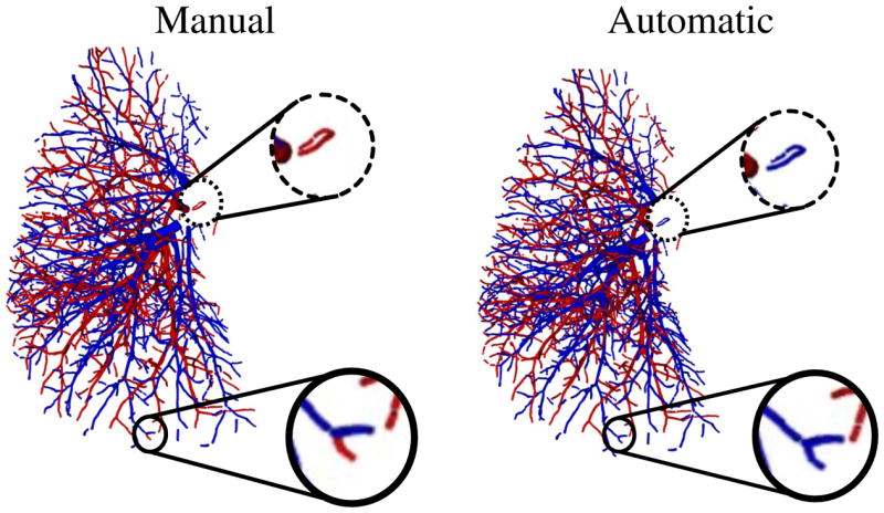
An example showing of isolated vessels (dotted circle) that are wrongly segmented by the automatic algorithm (right) in comparison with manual segmentation (left). The same case presents an example where the proposed automatic algorithm improves manual segmentation (full circle).

While using 2.5D patches the CNN seems to require information from both the CT image and the bronchus- and vessel-enhanced images (accuracy = ~82% when using only the CT image, accuracy = ~87% when including the enhanced images), a 3D CNN can learn all the necessary information from the CT image alone. Although we provided connectivity information to the 2.5D patches by including the two closest vessel points, the usage of 3D patches appears to provide the network with vessel segments that contain more local and global information for A/V separation. Moreover, the inclusion of images with enhanced vessels and bronchi does not improve the results for 3D patches. This suggests that the extra complexity of pre-computing feature enhanced images is not necessary as the 3D CNN approach can extract the relevant features.

For completeness, we also conducted an additional experiment to investigate the performance of the proposed 3D network on patches of 32×32×32 pixels extracted around the particle point without reformatting the plane along the vessel direction. For this particular case, isotropic convolutional filters of 7×7×7 pixels were used. Results on both lobes of the COPDGene cases showed that with this configuration the performance of our method worsens, both before and after applying GC. A mean accuracy of 83.6% (median accuracy: 84%, range: 69% to 95%), with a sensitivity and a specificity of 88.9% and 77.5%, respectively, was obtained after GC, while the use of the CNN only yields to a mean accuracy of 74.3% (median: 75%, range: 62% to 86%), with a sensitivity of 78.1% and a specificity of 69.9%. This demonstrates that considering small vessel segments along the vessel direction provides the network with optimal information for the purpose of A/V segmentation.

To motivate the choice of using CNN as the initial classifier, we also compared the performance of CNN against an RF approach which uses airway segmentation to define proximity of arteries to bronchi. The results showed that a CNN approach achieves higher results both in terms of overall classification (after GC) and as single classifier. Our CNN approach is an optimal starting point for the specific task of A/V separation on chest CT images without the need of explicitly segmenting airways, which might be a complex and error-prone process in disease cases like advanced emphysema.

To date, the only reliable comparison that can be accomplished with other methods available in the literature is with the approach recently presented in [16], where a publicly available challenge dataset for evaluating A/V separation algorithms has been proposed. The results on the subset of ten fully annotated cases, and of the reference and consensus set obtained on the 2,750 segments randomly selected from all 55 cases show that our algorithm outperforms the one in [16]. An important aspect to take into account is that results were obtained considering the whole lung for all considered cases. This demonstrates that the CNN well generalizes results despite being trained on only two lobes.

Moreover, in [16] an additional test on CT images of patients with COPD was also performed. In particular, a subset of 25 patients, seven of which were diagnosed with COPD with the remaining eighteen patients diagnosed as not having COPD, were considered. A mean accuracy of 88.57% was reported for the cases with COPD, while an accuracy of 88.56% was achieved for the no-COPD group. Although a direct comparison is not possible, as these cases are not publicly available, the eighteen cases considered for evaluation in this work (Section IV-A) were extracted from the COPDGene study and sixteen of them were diagnosed as having COPD. In these cases our algorithm yields to a mean accuracy of 93.6%, outperforming [16]. Since the same mean accuracy was obtained for the ten fully annotated cases provided by [16], which to the best of our knowledge were diagnosed as not having COPD, our algorithm seems to be reliable regardless the presence of disease in the lung, and it can be considered a good candidate for the investigation of morphological changes in the arteries and veins of patients with and without COPD. However, an important study to accomplish in the future is the evaluation of the algorithm for varying imaging parameters, such as slice thickness, reconstruction kernels, and radiation dose, to demonstrate the reliability of the algorithm under different imaging conditions.

Although a direct comparison is not possible, the approach we propose also seems to outperform the method described in [12], where an overall accuracy of 91.1% is reported. Moreover, while the method in [12] requires a bronchus-enhanced image to compute an arterialness measure, which is very sensitive to the quality of the enhancement and the parameters used, we use the CNN to solve parameter optimization and to let the network automatically learn the proximity of arteries to veins. This highly reduces the complexity of the algorithm and sensitivity to the chosen parameters.

An additional test we performed to evaluate the results on the vessels sub-divided into three groups based on their scale (Section IV-D), shows that the algorithm fails more in the large vessels, while it is optimal in the particles of medium size. This may be explained by the fact that for some points a patch size of 32×32 pixels may not be large enough to include all information necessary to distinguish arteries from veins. Also, due to the anatomy of the lung vessels, the training set is richer in medium size vessels than in large ones. Another important aspect to take into account is that the analysis of the results obtained before and after implementing GC indicates that while the CNN can well separate arteries from veins for central vessels, GC seems to have a key role for peripheral vessels. This may be due to the gradual vanishing of relevant information, such as the presence of airways in the proximity of arteries while moving toward the periphery. A possible solution to overcome these issues is an independent classification of the three groups, also applying a volume down-sampling to the patches of the large vessels to make the whole process scale-invariant.

To better understand the results on the COPDGene cohort, we also sub-divided the subjects based on the presence of COPD (4 cases with mild COPD, 10 cases with moderate COPD, and 4 cases with advanced COPD) and the presence of emphysema (12 subjects with the disease, 6 without). It is important to point out that two of the three cases used for training presented mild COPD and one had moderate COPD, while only one subject had emphysema. As shown in Tab. VI, the proposed method seems to be affected by a strong presence of COPD, while mild and moderate COPD and emphysema do not seem to affect much the performance of the algorithm. Moreover, the presence of disease affects more the specificity than the sensitivity of the algorithm, which decreases compared to control cases. This may suggest that using more cases with the presence of COPD and emphysema for training the CNN might help better generalize results.

TABLE VI.

Results (mean accuracy (in %) ± standard deviation) obtained on the validation cases from the COPDGene cohort with subjects sub-divided based on the presence of COPD and on the presence of emphysema. n indicates the number of patients for each group.

	Mild COPD (n=4)	Mod. COPD (n=10)	Adv. COPD (n=4)	Emph. (n=12)	No Emph. (n=6)
Mean Acc.	95.3 ± 2.3	94.6 ± 3.3	91.5 ± 7.5	92.6 ± 5.5	95.4 ± 2.1
Sensitivity	95.8 ± 3.1	98.2 ± 0.9	97.5 ± 1.6	97.2 ± 2.7	97.7 ± 2.1
Specificity	94.5 ± 2.2	90.1 ± 6.5	84.5 ± 15.7	87.1 ± 10.5	92.7 ± 3.0

To further validate the proposed method, we lastly compared the classification obtained with the proposed method on thirty-three CT contrast images from the CTEPH cohort. The obtained results indicate that the algorithm is reliable across different scan protocols and it is insensitive to the presence of contrast in the image. As expected, accuracy is higher in cases without disease, as CTEPH may distort the lung and vascular anatomy that may complicate distinction of arteries from veins. However, these results are encouraging as they demonstrate the ability of the algorithm to generalize the A/V classification regardless of the contrast in the image. Moreover, improved results may certainly be achieved by including contrast CT cases into the training set.

The obtained results also showed that the proposed architecture has a higher sensitivity (~97% for the COPDGene cohort, ~93% for the CTEPH cases) than specificity (~89% for COPDGene, ~84% for CTEPH), with the imbalance mainly introduced by GC (sensitivity and specificity for CNN on COPDGene cases before GC: ~84% and ~74%, respectively), probably based on the connectivity assumptions made to construct the graph. To avoid this issue and potentially improve results, a further opportunity for future work is to modify the last iterative step of the proposed GC to connect isolated subtrees with an integer program, similar to [12], to take into account more local and global structural information, and not only connected component, to construct the final graph.

Finally, from an analysis of the available data, the various datasets we used for evaluating the proposed algorithm always presented more arteries than veins (mean difference = 3, 625.38 ± 2, 508.53). This is consistent with the difference that has been shown in physiological studies of the pulmonary morphology in post-mortem analysis [35]. However, more investigations are needed to define how lung injury affects arterial and venous volumes.

VI. Conclusions

In this work, we have presented a novel fully automatic algorithm that utilizes a CNN approach combined with graphcuts optimization to separate arteries and veins in chest CT images. We compared different CNN architectures to the one proposed, training the network with both 2D and 3D patches that we extracted and integrated using different strategies. Since the classification is done on independent particles, which define the vessel candidates but do not provide connectivity information, we employed a GC approach to refine the segmentation and reduce any spatial inconsistency that may occur.

We showed that a 3D CNN can learn specific A/V characteristics from small vessel segments directly extracted from non-contrast CT images, and no further operations (i.e., bronchi and vessel enhancement, segmentation, etc.), are necessary. Our method outperforms the most recent algorithms proposed in [16] and [12], in comparison with the performance of human observers. Also, compared to [16], our approach yields higher performance for images of patients diagnosed both with and without COPD. Moreover, validation on the full lung of contrast CT images showed that the proposed trained method could be generalized to other modalities and it is reasonably insensitive to contrast and acquisition protocol variation.

In general, our results are promising and pave the way to future use of 3D CNN for A/V classification in CT images.

References

- 1.Coxson HO, Rogers RM. Quantitative computed tomography of chronic obstructive pulmonary disease. Acad Radiol. 2005;12(11):1457–1463. doi: 10.1016/j.acra.2005.08.013. [DOI] [PubMed] [Google Scholar]
- 2.Sluimer I, Schilham A, Prokop M, van Ginneken B. Computer analysis of computed tomography scans of the lung: a survey. IEEE Trans Med Imag. 2006;25(4):385–405. doi: 10.1109/TMI.2005.862753. [DOI] [PubMed] [Google Scholar]
- 3.Zhou C, Chan HP, Sahiner B, Hadjiiski LM, Chughtai A, Patel S, Wei J, Ge J, Cascade PN, Kazerooni EA. Automatic multiscale enhancement and segmentation of pulmonary vessels in CT pulmonary angiography images for CAD applications. Med Phys. 2007;34(12):4567–4577. doi: 10.1118/1.2804558. [DOI] [PMC free article] [PubMed] [Google Scholar]
- 4.Rahaghi FN, Ross JC, Agarwal M, González G, Come CE, Diaz AA, Vegas-Sánchez-Ferrero G, Hunsaker A, San José Estépar R, Waxman AB, et al. Pulmonary vascular morphology as an imaging biomarker in chronic thromboembolic pulmonary hypertension. Pulm Circ. 2016;6(1):70–81. doi: 10.1086/685081. [DOI] [PMC free article] [PubMed] [Google Scholar]
- 5.San José Estépar R, Kinney GL, Black-Shinn JL, Bowler RP, Kindlmann GL, Ross JC, Kikinis R, Han MK, Come CE, Diaz AA, et al. Computed tomographic measures of pulmonary vascular morphology in smokers and their clinical implications. American journal of respiratory and critical care medicine. 2013;188(2):231–239. doi: 10.1164/rccm.201301-0162OC. [DOI] [PMC free article] [PubMed] [Google Scholar]
- 6.Rahaghi FN, Wells JM, Come CE, Isaac A, Bhatt SP, Ross JC, Vegas-Sánchez-Ferrero G, Diaz AA, Minhas J, Dransfield MT, et al. Arterial and venous pulmonary vascular morphology and their relationship to findings in cardiac magnetic resonance imaging in smokers. J Comput Assist Tomo. 2016;40(6):948–952. doi: 10.1097/RCT.0000000000000465. [DOI] [PMC free article] [PubMed] [Google Scholar]
- 7.Lesage D, Angelini ED, Bloch I, Funka-Lea G. A review of 3d vessel lumen segmentation techniques: Models, features and extraction schemes. Med Im An. 2009;13(6):819–845. doi: 10.1016/j.media.2009.07.011. [DOI] [PubMed] [Google Scholar]
- 8.Bülow T, Wiemker R, Blaffert T, Lorenz C, Renisch S. Automatic extraction of the pulmonary artery tree from multi-slice CT data. Proc of SPIE Vol. 2005;5746:731. [Google Scholar]
- 9.Mekada Y, Nakamura S, Ide I, Murase H, Otsuji H. Pulmonary artery and vein classification using spatial arrangement features from x-ray ct images. Proc. 7th Asia-pacific Conference on Control and Measurement; 2006. pp. 232–235. [Google Scholar]
- 10.Saha PK, Gao Z, Alford SK, Sonka M, Hoffman EA. Topomorphologic separation of fused isointensity objects via multiscale opening: Separating arteries and veins in 3-D pulmonary CT. IEEE Trans Med Imag. 2010;29(3):840–851. doi: 10.1109/TMI.2009.2038224. [DOI] [PMC free article] [PubMed] [Google Scholar]
- 11.Gao Z, Grout RW, Holtze C, Hoffman EA, Saha P. A new paradigm of interactive artery/vein separation in noncontrast pulmonary ct imaging using multiscale topomorphologic opening. IEEE Trans on Biomed Eng. 2012;59(11):3016–3027. doi: 10.1109/TBME.2012.2212894. [DOI] [PMC free article] [PubMed] [Google Scholar]
- 12.Payer C, Pienn M, Balint Z, Shekhovtsov A, Talakic E, Nagy E, Olschewski A, Olschewski H, Urschler M. Automated integer programming based separation of arteries and veins from thoracic CT images. Med Im An. 2016;34:109–122. doi: 10.1016/j.media.2016.05.002. [DOI] [PubMed] [Google Scholar]
- 13.Park Sangmin, Bajaj Chandrajit L, Gladish Gregory. Artery-vein separation of human vasculature from 3d thoracic ct angio scans. CompIMAGE. 2006:331–336. [Google Scholar]
- 14.Park S, Min-Lee S, Kim N, Beom-Seo J, Shin H. Automatic reconstruction of the arterial and venous trees on volumetric chest ct. Med Phys. 2013;40(7) doi: 10.1118/1.4811203. [DOI] [PubMed] [Google Scholar]
- 15.Kitamura Y, Li Y, Ito W, Ishikawa H. Data-dependent higher-order clique selection for artery–vein segmentation by energy minimization. International Journal of Computer Vision. 2016;117(2):142–158. [Google Scholar]
- 16.Charbonnier JP, Brink M, Ciompi F, Scholten ET, Schaefer-Prokop CM, Van Rikxoort EM. Automatic pulmonary artery-vein separation and classification in computed tomography using tree partitioning and peripheral vessel matching. IEEE Trans Med Imag. 2016;35(3):882–892. doi: 10.1109/TMI.2015.2500279. [DOI] [PubMed] [Google Scholar]
- 17.LeCun Y, Bengio Y, Hinton G. Deep learning. Nature. 2015;521(7553):436–444. doi: 10.1038/nature14539. [DOI] [PubMed] [Google Scholar]
- 18.Boykov Y, Veksler O, Zabih R. Fast approximate energy minimization via graph cuts. IEEE T Pattern Anal. 2001;23(11):1222–1239. [Google Scholar]
- 19.Boykov Y, Veksler O. Graph cuts in vision and graphics: Theories and applications. Handbook of mathematical models in computer vision. 2006:79–96. [Google Scholar]
- 20.Kindlmann GL, San José Estépar R, Smith SM, Westin CF. Sampling and visualizing creases with scale-space particles. IEEE T Vis Comput Gr. 2009;15(6) doi: 10.1109/TVCG.2009.177. [DOI] [PMC free article] [PubMed] [Google Scholar]
- 21.San José Estépar R, Ross JC, Russian K, Schultz T, Washko GR, Kindlmann GL. Computational vascular morphometry for the assessment of pulmonary vascular disease based on scale-space particles. ISBI, 2012 9th IEEE Int. Symp. on; IEEE; 2012. pp. 1479–1482. [DOI] [PMC free article] [PubMed] [Google Scholar]
- 22.Nardelli P, Jimenez-Carretero D, Bermejo-Peláez D, Ledesma-Carbayo MJ, Rahaghi Farbod N, San José Estépar R. Deep-learning strategy for pulmonary artery-vein classification of non-contrast CT images. ISBI, 2017 14th IEEE Int. Symp. on; IEEE; 2017. pp. 384–387. [DOI] [PMC free article] [PubMed] [Google Scholar]
- 23.Regan EA, Hokanson JE, Murphy JR, Make B, Lynch DA, Beaty TH, Curran-Everett D, Silverman EK, Crapo JD. Genetic epidemiology of copd (copdgene) study design. COPD. 2011;7(1):32–43. doi: 10.3109/15412550903499522. [DOI] [PMC free article] [PubMed] [Google Scholar]
- 24.Breiman L. Random forests. Machine learning. 2001;45(1):5–32. [Google Scholar]
- 25.Ross JC, San José Estépar R, Díaz AA, Westin CF, Kikinis R, Silverman EK, Washko GR. MICCAI2009. Springer; 2009. Lung extraction, lobe segmentation and hierarchical region assessment for quantitative analysis on high resolution computed tomography images; pp. 690–698. [DOI] [PMC free article] [PubMed] [Google Scholar]
- 26.Frangi AF, Niessen WJ, Vincken KL, Viergever MA. MICCAI1998. Springer; 1998. Multiscale vessel enhancement filtering; pp. 130–137. [Google Scholar]
- 27.Jimenez-Carretero D. PhD thesis, Telecomunicacion. 2015. Pulmonary Artery-Vein Segmentation in Real and Synthetic CT Image. [Google Scholar]
- 28.Bondy JA, Murty USR. Graph theory with applications. Vol. 290. Macmillan; London: 1976. [Google Scholar]
- 29.Ross James C, Estépar Raúl San José, Díaz Alejandro, Westin Carl-Fredrik, Kikinis Ron, Silverman Edwin K, Washko George R. Lung extraction, lobe segmentation and hierarchical region assessment for quantitative analysis on high resolution computed tomography images. International Conference on Medical Image Computing and Computer-Assisted Intervention; Springer; 2009. pp. 690–698. [DOI] [PMC free article] [PubMed] [Google Scholar]
- 30.Kruskal JB. On the shortest spanning subtree of a graph and the traveling salesman problem. P Am Math Soc. 1956;7(1):48–50. [Google Scholar]
- 31.Rahaghi FN, Come CE, Ross JC, Harmouche R, Diaz AA, San Jose Estepar R, Washko G. Morphologic Response of the Pulmonary Vasculature to Endoscopic Lung Volume Reduction. COPD (Miami, Fla) 2015;2(3):214–222. doi: 10.15326/jcopdf.2.3.2014.0164. [DOI] [PMC free article] [PubMed] [Google Scholar]
- 32.Chollet F. Keras. 2015 https://github.com/fchollet/keras.
- 33.Abadi M, Agarwal A, Barham P, Brevdo E, Chen Z, Citro C, Corrado GS, Davis A, Dean J, Devin M, et al. Tensorflow: Large-scale machine learning on heterogeneous distributed systems. 2016 arXiv preprint arXiv:1603.04467. [Google Scholar]
- 34.Abadi M, Barham P, Chen J, Chen Z, Davis A, Dean J, Devin M, Ghemawat S, Irving G, Isard M, et al. Tensorflow: A system for large-scale machine learning. OSDI. 2016;16:265–283. [Google Scholar]
- 35.Huang Wei, Yen RT, McLaurine M, Bledsoe G. Morphometry of the human pulmonary vasculature. Journal of applied physiology. 1996;81(5):2123–2133. doi: 10.1152/jappl.1996.81.5.2123. [DOI] [PubMed] [Google Scholar]