Bias From Potentially Mischievous Responders on Large-Scale Estimates of Lesbian, Gay, Bisexual, or Questioning (LGBQ)–Heterosexual Youth Health Disparities

Abstract

Objectives. To determine how sensitive estimates of lesbian, gay, bisexual, or questioning (LGBQ)–heterosexual youth health disparities are to the presence of potentially mischievous responders.

Methods. We used US data from the 2015 Youth Risk Behavior Survey, pooled across jurisdictions that included a question about sexual identity for a total sample of 148 960 students. We used boosted regressions (a machine-learning technique) to identify unusual patterns of responses to 7 screener items presumably unrelated to LGBQ identification, which generated an index of suspected mischievousness. We estimated LGBQ–heterosexual youth disparities on 20 health outcomes; then we removed 1% of suspected mischievous responders at a time and re-estimated disparities to assess the robustness of original estimates.

Results. Accounting for suspected mischievousness reduced estimates of the average LGBQ–heterosexual youth health disparity by up to 46% for boys and 23% for girls; however, screening did not affect all outcomes equally. Drug- and alcohol-related disparities were most affected, particularly among boys, but bullying and suicidal ideation were unaffected.

Conclusions. Including screener items in public health data sets and performing rigorous sensitivity analyses can support the validity of youth health estimates.

Valid findings are the bedrock of scientific advancements. Whereas threats to validity such as replication failure^1,2 have garnered much attention from the scientific community, other, perhaps more prevalent, threats have gone relatively unmentioned in public health. We focus here on threats attributable to “mischievous responders”—respondents who mislead researchers by providing extreme and untruthful responses to multiple items, perhaps because they find it “funny” to do so^3–5—and the bias they introduce into health estimates. Mischievous responders intentionally overreport unusual and often undesirable behaviors, do so in patterned rather than haphazard ways, and disproportionately (falsely) claim to be minority youths.^3–5 Thus, mischievous responder bias is distinct from well-known threats to validity, such as recall error, underreporting stigmatized or illegal behaviors, or apathetically providing random answers,^6,7 and may be a more serious threat than the others for research on minority youths. Here, we examined how potentially mischievous responders can bias comparisons of youth health along the dimension of sexual identity. That is, we estimated the effects of potentially mischievous responders on a range of health outcomes comparing youths who identify as lesbian, gay, bisexual, or questioning (LGBQ) with heterosexual-identified youths via anonymous self-administered questionnaires. The topic of mischievous responders and the novel approach we propose for identifying them have broad implications for health, social, and psychological science comparisons of groups on the basis of race/ethnicity, gender identity, citizenship, disability status, and more.

By comparison with other data-gathering methods such as interviews, self-administered questionnaires are inexpensive, easy to administer, and can preserve anonymity when gathering sensitive health and sexuality data.^8–11 Thus, it is not surprising that they provide a core method of obtaining nationally representative data used to support policy and represent the principal mode for gathering large-scale data on LGBQ youths.^12–15 Despite the obvious benefits of this mode of data collection, a growing number of studies calls into question the validity of these data,^4,5,16–18 raising concerns that mischievous responders may masquerade as extremely risky and deviant LGBQ youths on self-administered questionnaires and distort the results of research based on such data.⁵

Previous attempts to identify mischievous responders relied largely on verifying youth responses on self-administered questionnaires with parent reports or in-person follow-ups³ or asking respondents if they answered all questions honestly.¹⁹ Parental interviews, for instance, revealed that 19% of “adopted” youth in fact were not adopted.³ Similarly, in-person follow-ups revealed that 99% of “amputee” youth had all limbs,³ and 12% of youth admitted not answering all items honestly.¹⁹ Although it may work well to ask parents whether their children were adopted,³ it would be unethical to ask parents to verify their child’s reported sexuality. Also, verification—parental or in-person—is often expensive and cannot be done anonymously, and asking youths whether they responded honestly may not yield an honest response.

We propose a novel approach to identifying potentially mischievous responders in existing large data sets by using machine-learning techniques to identify unusual patterns of responses to screener items (e.g., frequency of eating carrots, height) presumably unrelated to LGBQ identification on self-administered questionnaires. After identifying the most likely mischievous youths, we can assess the robustness of estimates of LGBQ–heterosexual youth health disparities to the inclusion of the suspect data.

METHODS

We utilized a large public health data set first to identify potentially mischievous responders, and then to examine how the inclusion of these mischievous responders may have an impact on estimates of LGBQ health disparities. Several follow-up analyses refined this analysis by examining the sensitivity of specific health outcomes to potentially mischievous responders as well as the sensitivity of the approach to the composition of the screener items.

Data

We used data from the YRBS, which has contributed to a large literature base^20–24 and is publicly available from the Centers for Disease Control and Prevention: https://www.cdc.gov/healthyyouth/data/yrbs/data.htm. For the main analysis, we restricted the weighted data to states and districts from the 2015 wave of data collection (with a beginning n = 197 416) with nonmissing values for sex (reducing to n = 195 769) and sexual identity (reducing to n = 148 960). The large reduction attributable to the sexual identity item was because many locations did not include that item on their survey (Text A, available as a supplement to the online version of this article at http://www.ajph.org, for these locations). This final analytic sample included 72 641 male participants and 76 319 female participants.

Locations participating in the publicly released State and District 2015 YRBS that also asked the sexual identity item included 20 states (Arizona, Arkansas, California, Connecticut, Delaware, Florida, Illinois, Kentucky, Maine, Maryland, Michigan, Nevada, New York, North Carolina, North Dakota, Oklahoma, Pennsylvania, Rhode Island, West Virginia, and Wyoming) and 11 districts (Bronx, NY; Brooklyn, NY; Broward County, FL; Duval County, FL; Manhattan, NY; Miami–Dade County, FL; New York City, NY; Orange County, FL; Queens, NY; San Diego, CA; and Staten Island, NY).

Following the analysis of the pooled State and District 2015 YRBS, we performed a preregistered replication analysis (https://aspredicted.org/6mp9r.pdf) on the National 2015 YRBS (n = 14 612).

Outcomes

The YRBS asked high-school students a range of questions relating to risk-taking behaviors and attitudes. We selected 20 items commonly examined in the LGBQ literature as outcomes for our study (see the User’s Guide²⁵ for specific phrasing of items): rode in a car with a drunk driver, drove drunk, skipped school because felt unsafe, fought at school, was forced into sex, their partner forced sex on them, was bullied at school, felt sad/hopeless, considered suicide, planned suicide, attempted suicide, smoking, alcohol use, cocaine use, heroin use, ecstasy use, steroids use, number of sexual partners, physical activity, and TV watching.

We coded outcomes continuously (e.g., reporting “20 to 39 times” was coded as 29.5), and we also ran specification checks to test if the patterns persisted when outcomes were instead coded dichotomously (i.e., some risk vs no risk).

Identification of Potentially Mischievous Responders

To identify potentially mischievous responders, we exploited the relationships between reporting being LGBQ and responses to other survey items that are ostensibly unrelated to actually being LGBQ. For example, we would expect that no meaningful relationship exists between sexuality and the frequency with which an individual eats carrots, fruit, salads, or potatoes. Similarly, we expect that height, asthma, and dentist visits are not associated with sexuality. Thus, we would expect that a logistic regression predicting sexuality (LGBQ vs heterosexual) as a function of height, asthma, dentist visits, and eating habits would not predict sexuality. However, these predictor items share a common feature with sexuality on self-administered questionnaires—they all contain response options that some youths would find funny to answer affirmatively.^4,5,16 For example, a mischievous responder might find it funny to report that he eats carrots, fruit, potatoes, and salads each “four or more times a day”; is extremely tall; is unsure whether he has asthma; has never been to the dentist; and that he identifies as “gay,” even if none of these is true for this individual in reality. Thus, the presence of mischievous responders creates spurious relationships between these predictor (screener) items and sexuality that would not otherwise exist if all individuals were responding truthfully. We capitalized on these spurious relationships to identify youths providing the most unusual patterns of responses to these other survey items that we use as a screener, then estimated what disparities in health outcomes were without these individuals in the analysis.

We used boosted regressions²⁶ (a machine-learning technique) to predict reporting LGBQ identification as a function of the screener items (e.g., carrot eating, height). We arrived at the functional form of the boosted regression through a computationally intensive cross-validation procedure that allows for the iterative discovery of higher-level interactions among predictors to better estimate the dependent variable.^26,27 Such advanced machine-learning techniques are gaining popularity in applied statistics and economics for their efficiency in identifying complex relationships and for the cross-validation procedures used to identify these relationships, which rely on fewer researcher assumptions about the functional form.^27–29 Thus, although this approach requires researchers to choose the items to include in the screener, it does not require researchers to identify which outcome responses may be tempting to mischievous responders, nor how these items relate to one another.^26–29 The model to be discovered via boosted regression was

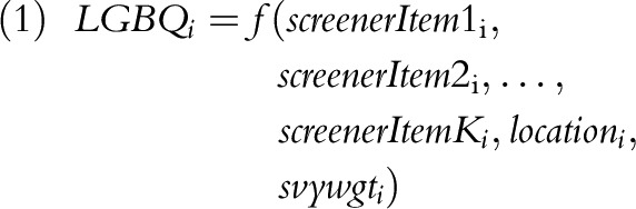where i indexes individual respondents, K is the number of screener items used (7 in the main analysis, though we varied K to 1, 5, 6, and 8 in supplemental analyses), and location fixed effects account for jurisdictions being allowed to select which items to include (so that this selection did not affect potential mischievous responder identification for other locations; however, note that supplemental analyses revealed that locations themselves did not alter estimates of LGBQ–heterosexual disparities in the screening process). We included survey weights as predictors in this stage.³⁰

The boosted logistic regression generated a propensity²⁷ for each individual to report being “LGBQ” on the basis of their unique response combination to the ostensibly unrelated screener items. These propensities served as proxies for the likelihood an individual is a mischievous responder. Table 1 shows how screening based on these propensities altered the proportion of youths reporting LGBQ identities in the main sample. Table 1 also illustrates that screening did not substantially alter the race/ethnicity, age, or grade representations of the YRBS sample, and thus is unlikely to meaningfully affect generalizability. Supplemental validity checks confirmed that the boosted regressions did in fact identify unusual, low-probability responses and response combinations (Figures A–P, available as supplements to the online version of this article at http://www.ajph.org). All analyses were performed separately by reported sex.

TABLE 1—

Demographic Characteristics of the Weighted Sample Among Boys and Girls by Screener Threshold: Pooled Youth Risk Behavior Survey, United States, 2015

	Boys (Unweighted n = 72 641)				Girls (Unweighted n = 76 319)
Characteristic	Full Sample, %	5% Screened Out, %	10% Screened Out, %	25% Screened Out, %	Full Sample, %	5% Screened Out, %	10% Screened Out, %	25% Screened Out, %
Sexual identity
Heterosexual	91.77	92.38	92.72	93.42	82.82	83.35	83.81	85.39
Gay or lesbian	2.49	2.35	2.27	2.08	2.07	2.02	1.98	1.84
Bisexual	2.88	2.66	2.56	2.38	9.94	9.66	9.38	8.31
Questioning	2.86	2.61	2.46	2.12	5.17	4.97	4.83	4.46
Race/ethnicity
White	46.58	46.94	47.28	48.10	45.12	45.89	45.91	45.89
Black or African American	14.62	14.39	14.16	13.21	15.55	15.14	14.98	14.23
Hispanic or Latino	27.14	27.08	26.98	27.19	28.32	28.10	28.27	29.10
All other races	11.66	11.59	11.59	11.50	11.02	10.87	10.84	10.78
Grade
9th	27.50	27.39	27.28	26.95	26.84	26.74	26.78	26.63
10th	25.75	25.81	25.77	25.55	25.62	25.62	25.59	25.68
11th	23.96	23.98	24.07	24.39	24.04	24.09	24.08	24.14
12th	22.78	22.82	22.89	23.11	23.50	23.55	23.55	23.55
Age, y
≤ 12	0.29	0.20	0.16	0.08	0.32	0.23	0.21	0.15
13	0.47	0.42	0.40	0.34	0.47	0.44	0.41	0.35
14	12.29	12.24	12.14	11.97	13.49	13.31	13.24	12.97
15	25.50	25.59	25.58	25.41	26.11	26.11	26.10	26.32
16	24.94	24.96	24.99	25.12	24.88	25.01	25.08	24.90
17	23.14	23.20	23.31	23.48	22.80	22.97	22.94	23.03
≥ 18	13.37	13.39	13.42	13.60	11.92	11.94	12.02	12.29

Note. Our sensitivity analysis approach was to remove a fixed number (i.e., unweighted amount) of observations at each removal step (e.g., 5% screened out, 10% screened out). The percentages in the table reflect the weighted sample that remains at each of the selected screening thresholds.

The Effects of Potentially Mischievous Responders

First, we estimated health disparities for 20 outcomes by using location fixed-effect regression models with the full data set. For all models, we obtained asymmetric percentile-t confidence intervals (CIs) via 1999 clustered bootstrapped replications, with resampling at the primary sampling unit and jurisdiction levels, to account for the complex sampling design and clustering of observations. Next, we removed the top 1% of cases in terms of likely mischievousness (i.e., cases exhibiting the most unusual response patterns to the screener items) and re-estimated health disparities with the remaining 99% of the data. Then, we proceeded to remove another 1% and re-estimate disparities again, and so on, to see whether the original estimate was robust to the removal of potentially mischievous responders and—if it was not robust—if and when the disparity estimates began to stabilize. The objective of our proposed procedure was not necessarily to remove data to arrive at the one “true” estimate, but rather to assess the stability or robustness of the original estimate to the possibility of mischievous responders. Instability suggests that caution is warranted in interpreting the original estimate.

In addition, we tested whether the change in the average disparity from the model with the full data set to a model with some observations removed was statistically significant, which indicates how sensitive estimates are to likely mischievous responders. To test for significant changes across models, we performed 1999 clustered bootstrapped replications of the entire process described to this point, including the boosted logistic regression. This bootstrapping process not only allowed us to test for significant differences across models but also had the added benefits of accounting for error in the propensity scores generated via the boosted regression and allowing us to estimate the covariance matrix across changes to adjust for when aggregating. Supplemental Text A provides technical details. In addition to looking at overall patterns in youth health disparities, we examined individual outcomes. The methods were the same as those described previously.

Response-Option Extremity

To advance theory on mischievous responding patterns and to better understand the attributes of outcomes most affected by mischievous responders, we examined whether the variation across the 20 outcomes was systematic and could be explained by a feature of the outcome items. Specifically, because mischievous responders are expected to choose the most extreme response options,^3–6,16 we hypothesized that outcomes with fewer respondents choosing the most extreme options would be most affected by attempts to remove mischievous responders. To test this hypothesis, we estimated a random-effects model predicting the change in the estimated outcome disparity as a function of the percentage of respondents choosing the most extreme response option. In addition, we tested whether this mechanistic explanation held when the continuously coded outcomes were recoded dichotomously as “no risk” versus “some risk.”

Sensitivity Checks and Supplemental Analyses

In addition to the primary questions, we performed 3 sets of supplemental analyses to assess the robustness of our findings. First, we estimated mischievousness effects by LGBQ-identification subgroup to see if all subgroups were affected equally by screening. Second, we added and removed screener items used to identify potentially mischievous responders to assess whether the items selected for inclusion in the original screener were unique in producing the pattern of results observed for changes in disparities, or whether similar patterns would have been observed with slightly different screener items. Third, we performed a preregistered replication of our main analyses with the National 2015 YRBS.

RESULTS

Table 2 illustrates that the average LGBQ–heterosexual youth health outcome disparity among boys was 0.37 SDs (95% CI = 0.29, 0.45) when we used all data, but reduced to 0.30 SDs (95% CI = 0.22, 0.39) when we removed the top 5% of observations identified by the boosted logistic regression, a significant reduction of 18% or 0.07 SDs (95% CI = 0.04, 0.09). The average disparity dropped further, to 0.27 SDs (95% CI = 0.18, 0.35), when we removed the top 10% of observations. That is, removing the 10% of youths who provided the most unusual patterns of responses to items such as height, vegetable eating, and dentist visits reduced average estimates of LGBQ–heterosexual male health disparities by about 28% from the original estimate, a significant reduction of 0.11 SDs (95% CI = 0.07, 0.14). Removing the top 25% left the average disparity at 0.20 SDs (95% CI = 0.11, 0.29), a reduction of 46% or 0.17 SDs (95% CI = 0.11, 0.23).

TABLE 2—

Estimated Average Lesbian, Gay, Bisexual, and Questioning–Heterosexual Youth Health Disparities Across 20 Outcomes: Pooled Youth Risk Behavior Survey, United States, 2015

	Average LGBQ–Heterosexual Disparity, B (95% CI)	Difference in Average Disparity,a B (95% CI)
Boys
Full sample	0.37 (0.29, 0.45)	. . .
1% screened	0.35 (0.26, 0.43)	0.03 (0.02, 0.03)
5% screened	0.30 (0.22, 0.39)	0.07 (0.04, 0.09)
10% screened	0.27 (0.18, 0.35)	0.11 (0.07, 0.14)
15% screened	0.23 (0.15, 0.32)	0.14 (0.09, 0.19)
20% screened	0.21 (0.13, 0.30)	0.16 (0.10, 0.21)
25% screened	0.20 (0.11, 0.29)	0.17 (0.11, 0.23)
Girls
Full sample	0.31 (0.23, 0.38)	. . .
1% screened	0.30 (0.22, 0.37)	0.01 (0.00, 0.02)
5% screened	0.27 (0.19, 0.35)	0.04 (0.02, 0.06)
10% screened	0.25 (0.17, 0.33)	0.06 (0.03, 0.08)
15% screened	0.24 (0.15, 0.32)	0.07 (0.04, 0.10)
20% screened	0.24 (0.15, 0.32)	0.07 (0.04, 0.10)
25% screened	0.24 (0.15, 0.32)	0.07 (0.03, 0.11)

Note. CI = confidence interval; LGBQ = lesbian, gay, bisexual, and questioning. All estimates are reported as standardized differences and can be interpreted using typical effect size standards. All estimates (both overall and difference) are statistically significant at P < .004. This table presents a concise subset of screening values; see Table A (available as a supplement to the online version of this article at http://www.ajph.org) for similar information for each percentage of students screened up to 25%. Male n = 72 641 (6909 LGBQ). Female n = 76 319 (14 142 LGBQ).

^aDifference in average disparity from model using the full sample to a model using a screened sample.

Changes in average disparities among girls followed a similar albeit attenuated pattern, dropping an average of 13% or 0.04 SDs (95% CI = 0.02, 0.06) and 23% or 0.07 SDs (95% CI = 0.03, 0.11) when we removed 5% and 25% of the data, respectively. Also, the average estimates converged to a stable value (around 0.24 SDs) relatively quickly among girls, but failed to stabilize among boys (although some individual outcomes stabilized for boys [Figure 1], and the male average stabilized in a replication study). The attenuated pattern among girls was expected because research using a verification method found that male adolescents tend to be more mischievous, and a small subset of mischievous male adolescents even report being “female” while completing surveys, thus making female adolescents appear more mischievous than they are.³

FIGURE 1—

Estimated Lesbian, Gay, Bisexual, and Questioning (LGBQ)–Heterosexual Youth Health Disparities, by Outcome and Mischievous Responder Screening Threshold Among (a) Boys and (b) Girls: Pooled Youth Risk Behavior Survey, United States, 2015

Note. driv. = driver; Phys. activ. = Physical activity. Asymmetric percentile-t 95% confidence intervals were constructed from 1999 bootstrapped replications. If the 95% confidence interval (in gray) does not cross the horizontal red line at 0, the disparity is statistically significant (P < .05). Table B (available as a supplement to the online version of this article at http://www.ajph.org) provides a tabular version of the estimates for select screening values. Male n = 72 641 (6909 LGBQ). Female n = 76 319 (14 142 LGBQ).

Importantly, the reductions in disparity estimates observed for removing potentially mischievous responders were statistically significant when as little as 1% of the data were removed among both male and female participants (Table 2). Thus, even a very small group of potentially mischievous responders can bias estimates of LGBQ–heterosexual youth health disparities.

Screening Does Not Affect All Outcomes Equally

While Table 2 presents how the disparities look on average, the 20 outcomes exhibited substantial variation in the extent to which they were affected by potentially mischievous responders (Figure 1). Estimates related to drug- and alcohol-use disparities were more affected than were those related to bullying and most suicide-related disparities, especially among boys. For example, the male LGBQ–heterosexual ecstasy-use disparity reduced from 0.31 SDs (95% CI = 0.08, 0.71) in the full data set to 0.04 SDs (95% CI = −0.08, 0.18) when we removed the top 25% of responders, a significant drop of 87% or 0.27 SDs (95% CI = 0.10, 0.64). By contrast, the male LGBQ–heterosexual disparity in being bullied at school was virtually unchanged, from 0.39 SDs (95% CI = 0.22, 0.57) to 0.38 SDs (95% CI = 0.15, 0.61). Thus, it is highly unlikely that mischievous responders were responsible for disparities in bullying and most suicide-related outcomes (Figure 1), but they may have contributed considerably to disparities in substance use, to the point where many substance-use disparities became statistically nonsignificant. Estimated changes in any individual outcome were less precise than were changes on average. Also, individual outcomes for girls were less affected by screening.

Response-Option Extremity and Mischievousness Differences

Analyses in Figure 2 provided strong support for the hypothesis that outcomes with fewer respondents choosing extreme options are more susceptible to mischievous responder bias, with B = 0.75 (95% CI = 0.59, 0.91) among boys and B = 0.75 (95% CI = 0.54, 0.95) among girls. This helps explain why some outcomes were more affected by screening than were other outcomes. These relationships persisted even if the outcomes were dichotomized to “no risk” versus “some risk,” with coefficients of B = 0.67 (95% CI = 0.42, 0.91) among boys and B = 0.75 (95% CI = 0.48, 1.01) among girls. In fact, all of the patterns discussed thus far were robust to outcome dichotomization (Figure Q, available as a supplement to the online version of this article at http://www.ajph.org). This suggests that many of the individuals selecting these low-frequency, high-risk response options were likely mischievous responders who had both exaggerated their extreme risk and falsely reported their sexuality. Moreover, they biased estimates regardless of whether the outcomes were coded continuously or dichotomously.

FIGURE 2—

Changes in Lesbian, Gay, Bisexual, and Questioning–Heterosexual Youth Item-Level Disparities Predicted by Item Response-Option Extremity Among (a) Boys and (b) Girls: Pooled Youth Risk Behavior Survey, United States, 2015

Note. Phys. activ. = Physical activity. For each sex, items to the left (with less frequently chosen extreme responses) are generally more susceptible to mischievous responder bias than are items to the right (with more frequently chosen extreme responses). Each random-effect model had 500 observations (20 outcome items times 25 percentiles at which disparities changes were estimated). Changes in disparities were predicted by item response-option extremity (natural-logged), indicators for percentage of data removed, and random effects for item. Robust SEs were adjusted for clustering at the item level. In the analyses, the item response-option extremity variable was natural-logged because of positive skew in the original, unlogged variable; for ease of interpretation, the unlogged values are presented in the figure.

^aProportion of respondents choosing the most extreme response option.

Sensitivity Checks and Supplemental Analyses

First among the supplemental analyses, results by LGBQ identification subgroup revealed almost no detectable differences in how potentially mischievous responders affected subgroups among male adolescents, but revealed substantial variation among female adolescents in how potentially mischievous responders affected the subgroups, with girls reporting “questioning” affected disproportionately by screening (Tables C–E, available as supplements to the online version of this article at http://www.ajph.org). Second, we found that the patterns of the effects for removing potentially mischievous responders were robust to changes in the composition of the screener itself (Figures R–T, available as supplements to the online version of this article at http://www.ajph.org), suggesting that the ultimate composition of the screener (1) is largely insensitive to the removal or addition of a small subset of items and (2) may be less consequential than whether researchers perform sensitivity analyses using any one of a set of reasonable screeners. Third, replication results with the National 2015 YRBS were largely consistent with those of the original analyses described previously (Figures U–V, available as supplements to the online version of this article at http://www.ajph.org). Texts B and C (available as supplements to the online version of this article at http://www.ajph.org) contain additional details about these supplemental analyses.

DISCUSSION

Our analyses revealed that potentially mischievous responders significantly affected overall estimates of LGBQ–heterosexual youth health disparities, especially among male youths, though some important disparities persisted. Drug- and alcohol-use disparities were among those most affected by suspect data, whereas disparity estimates for being bullied, feeling sad or hopeless, and thinking about suicide were not noticeably affected by suspect cases. These differential patterns of screening effects across outcomes were strongly and reliably predicted by how few respondents selected the most extreme outcome response options. All of these patterns were robust to screener modifications and replicated in a different, nationally representative data set.

We focused on data gathered via anonymous, in-school, self-administered questionnaires. The effects of screening are likely to vary across methodological and contextual dimensions.^5,6 For example, studies using Add Health—which assessed sexuality differently (attraction), following a face-to-face, nonanonymized, in-home questionnaire, and asked questions of the parent or guardian as part of the survey—may or may not find significant effects of screening.^6,31,32

PUBLIC HEALTH IMPLICATIONS

As demonstrated in this work, the inclusion of screener items in anonymous public health surveys provides an important opportunity to identify and remove potentially mischievous responders. Furthermore, following our example, we recommend that public health researchers estimate a series of disparities to assess sensitivity to different data-exclusion criteria. Although one can never be certain that the individuals identified as most likely to be mischievous responders are correctly identified, multiple model specifications and validity checks help ensure the integrity of the screening process and the conclusions drawn from the data. This process acknowledges the uncertainty in the estimates by using self-reported data and makes transparent the attempts to address the threat of mischievous responders. Moreover, using boosted regressions should yield more efficient and less assumption-laden identification of mischievous cases than previously used methods such as screening on a simple count of extreme responses⁵ or regression adjustment.³¹ Using the approach introduced in this article, researchers can take proactive steps to ensure the validity of their conclusions and of the public health policies they shape.

Our results related to outcome response-option extremity yield additional considerations at the survey development and results interpretation stages of public health research. That is, we found strong evidence that outcome items with high-risk, low-frequency response options (e.g., reporting using ecstasy “40 or more times”) were most affected by screening, and thus most likely influenced by mischievous responders. Understanding the types of outcome responses (e.g., high-risk combined with low-frequency) that mischievous responders are likely to select can help researchers in at least 2 ways. First, in the survey-development stage, researchers may consider altering outcome response options to reduce the options most attractive to mischievous responders. Second, in the results interpretation stage, exploring attributes of the outcome items themselves—specifically, item response-option extremity—may help researchers interpret why some of their outcomes are more affected by screening than are other outcomes.

To facilitate the use of screening analyses with the 2015 YRBS data, we make all of our main screening weights freely available for download from the Open Science Framework at https://osf.io/xkvgq, and Text D, available as a supplement to the online version of this article at http://www.ajph.org, explains how to use these weights. Thus, researchers can readily assess the robustness of their own findings with the 2015 YRBS data. Researchers working with other data sets can follow the procedures in this article to create their own screening weights. Because the literature on mischievous responders and screening techniques is still relatively nascent, we refrain from making strong suggestions concerning specific items to include in screeners or when to stop screening out observations. We reiterate, however, our recommendation of estimating a series of disparities and assessing stability in those estimates. As the field’s knowledge increases, guidelines for optimal screening may become clearer. Future research should continue to explore when, why, and how mischievous responders are influencing the robustness of estimates of health disparities.

REFERENCES

- 1.Fanelli D, Ioannidis JP. US studies may overestimate effect sizes in softer research. Proc Natl Acad Sci U S A. 2013;110(37):15031–15036. doi: 10.1073/pnas.1302997110. [DOI] [PMC free article] [PubMed] [Google Scholar]
- 2.Open Science Collaboration. Estimating the reproducibility of psychological science. Science. 2015;349(6251):aaac4716. doi: 10.1126/science.aac4716. [DOI] [PubMed] [Google Scholar]
- 3.Fan X, Miller BC, Park K-E et al. An exploratory study about inaccuracy and invalidity in adolescent self-report surveys. Field Methods. 2006;18(3):223–244. [Google Scholar]
- 4.Furlong MJ, Sharkey JD, Bates MP, Smith DC. An examination of the reliability, data screening procedures, and extreme response patterns for the Youth Risk Behavior Surveillance Survey. J Sch Violence. 2008;3(2-3):109–130. [Google Scholar]
- 5.Robinson-Cimpian JP. Inaccurate estimation of disparities due to mischievous responders: several suggestions to assess conclusions. Educ Res. 2014;43(4):171–185. [Google Scholar]
- 6.Cimpian JR. Classification errors and bias regarding research on sexual minority youths. Educ Res. 2017;46(9):517–529. [Google Scholar]
- 7.Groves RM, Jr, Fowler FJ, Couper MP, Lepkowski JM, Tourangeau R. Survey Methodology. Hoboken, NJ: John Wiley and Sons; 2011. [Google Scholar]
- 8.Badgett L. Best Practices for Asking Questions About Sexual Orientation on Surveys. Los Angeles, CA: Williams Institute; 2009. [Google Scholar]
- 9.Saewyc EM, Bauer GR, Skay CL et al. Measuring sexual orientation in adolescent health surveys; evaluation of eight school-based surveys. J Adolesc Health. 2004;35(4):345e1–345e15. doi: 10.1016/j.jadohealth.2004.06.002. [DOI] [PubMed] [Google Scholar]
- 10.Tourangeau R, Yan T. Sensitive questions in surveys. Psychol Bull. 2007;133(5):859–883. doi: 10.1037/0033-2909.133.5.859. [DOI] [PubMed] [Google Scholar]
- 11.Turner CF, Ku L, Rogers SM, Lindberg LD, Pleck JH, Sonenstein FL. Adolescent sexual behavior, drug use, and violence: increased reporting with computer survey technology. Science. 1998;280(5365):867–873. doi: 10.1126/science.280.5365.867. [DOI] [PubMed] [Google Scholar]
- 12.Kann L, Olsen EO, McManus T et al. Sexual identity, sex of sexual contacts, and health-related behaviors among students in grades 9–12—United States and selected sites, 2015. MMWR Surveill Summ. 2016;65(9):1–202. doi: 10.15585/mmwr.ss6509a1. [DOI] [PubMed] [Google Scholar]
- 13.Espelage DL, Aragon SR, Birkett M, Koenig BW. Homophobic teasing, psychological outcomes, and sexual orientation among high school students: what influence do parents and schools have? School Psych Rev. 2008;37(2):202–216. [Google Scholar]
- 14.Robinson JP, Espelage DL. Inequities in educational and psychological outcomes between LGBTQ and straight students in middle and high school. Educ Res. 2011;40(7):315–330. [Google Scholar]
- 15.Russell ST, Sinclair KO, Poteat VP, Koenig BW. Adolescent health and harassment based on discriminatory bias. Am J Public Health. 2012;102(3):493–495. doi: 10.2105/AJPH.2011.300430. [DOI] [PMC free article] [PubMed] [Google Scholar]
- 16.Furlong MJ, Fullchange A, Dowdy E. Effects of mischievous responding on universal mental health screening: I love rum raisin ice cream, really I do! Sch Psychol Q. 2017;32(3):320–335. doi: 10.1037/spq0000168. [DOI] [PubMed] [Google Scholar]
- 17.Jia Y, Konold TR, Cornell D, Huang F. The impact of validity screening on associations between self-reports of bullying victimization and student outcomes. Educ Psychol Meas. 2018;78(1):80–102. doi: 10.1177/0013164416671767. [DOI] [PMC free article] [PubMed] [Google Scholar]
- 18.Shukla K, Konold T. A two-step latent profile method for identifying invalid respondents in self-reported survey data. J Exp Educ. 2017;86(3):473–488. [Google Scholar]
- 19.Cornell D, Klein J, Konold T, Huang F. Effects of validity screening items on adolescent survey data. Psychol Assess. 2012;24(1):21–35. doi: 10.1037/a0024824. [DOI] [PubMed] [Google Scholar]
- 20.Centers for Disease Control and Prevention. YRBS journal articles by DASH authors. 2017. Available at: https://www.cdc.gov/healthyyouth/data/yrbs/pdf/yrbs_journal_articles_v3.pdf. Accessed October 22, 2017.
- 21.Clayton HB, Lowry R, August E, Jones SE. Nonmedical use of prescription drugs and sexual risk behaviors. Pediatrics. 2016;137(1):e20152480. doi: 10.1542/peds.2015-2480. [DOI] [PMC free article] [PubMed] [Google Scholar]
- 22.Raifman J, Moscoe E, Austin SB, McConnell M. Difference-in-differences analysis of the association between state same-sex marriage policies and adolescent suicide attempts. JAMA Pediatr. 2017;171(4):350–356. doi: 10.1001/jamapediatrics.2016.4529. [DOI] [PMC free article] [PubMed] [Google Scholar]
- 23.Vagi KJ, O’Malley Olsen E, Basile KC, Vivolo-Kantor AM. Teen dating violence (physical and sexual) among US high school students: findings from the 2013 national Youth Risk Behavior Survey. JAMA Pediatr. 2015;169(5):474–482. doi: 10.1001/jamapediatrics.2014.3577. [DOI] [PMC free article] [PubMed] [Google Scholar]
- 24.Zaza S, Kann L, Barrios LC. Lesbian, gay, and bisexual adolescents population estimate and prevalence of health behaviors. JAMA. 2016;316(22):2355–2356. doi: 10.1001/jama.2016.11683. [DOI] [PMC free article] [PubMed] [Google Scholar]
- 25.Centers for Disease Control and Prevention. 2015 YRBS Data User’s Guide. 2016. Available at: https://www.cdc.gov/healthyyouth/data/yrbs/pdf/2015/2015_yrbs-data-users_guide_smy_combined.pdf. Accessed February 16, 2017.
- 26.Friedman JH. Greedy function approximation: a gradient boosting machine. Ann Stat. 2001;29(5):1189–1232. [Google Scholar]
- 27.McCaffrey DF, Ridgeway G, Morral AR. Propensity score estimation with boosted regression for evaluating causal effects in observational studies. Psychol Methods. 2004;9(4):403–425. doi: 10.1037/1082-989X.9.4.403. [DOI] [PubMed] [Google Scholar]
- 28.Athey S, Imbens GW. The state of applied econometrics: causality and policy evaluation. J Econ Perspect. 2017;31(2):3–32. [Google Scholar]
- 29.Mullainathan S, Spiess J. Machine learning: an applied econometric approach. J Econ Perspect. 2017;31(2):87–106. [Google Scholar]
- 30.Dugoff EH, Schuler M, Stuart EA. Generalizing observational study results applying propensity score methods to complex surveys. Health Serv Res. 2014;49(1):284–303. doi: 10.1111/1475-6773.12090. [DOI] [PMC free article] [PubMed] [Google Scholar]
- 31.Fish JN, Russell ST. Have mischievous responders misidentified sexual minority youth disparities in the National Longitudinal Study of Adolescent to Adult Health? Arch Sex Behav. 2017 doi: 10.1007/s10508-017-0993-6. Epub ahead of print. [DOI] [PMC free article] [PubMed] [Google Scholar]
- 32.Savin-Williams RC, Joyner K. The dubious assessment of gay, lesbian, and bisexual adolescents of Add Health. Arch Sex Behav. 2014;43(3):413–422. doi: 10.1007/s10508-013-0219-5. [DOI] [PubMed] [Google Scholar]