Accurate Genomic Prediction of Human Height

Hsu et al. used advanced methods from machine learning to analyze almost half a million genomes. They produced, for the first time, accurate genomic predictors for complex traits such as height, bone density, and educational attainment...

Abstract

We construct genomic predictors for heritable but extremely complex human quantitative traits (height, heel bone density, and educational attainment) using modern methods in high dimensional statistics (i.e., machine learning). The constructed predictors explain, respectively, ∼40, 20, and 9% of total variance for the three traits, in data not used for training. For example, predicted heights correlate ∼0.65 with actual height; actual heights of most individuals in validation samples are within a few centimeters of the prediction. The proportion of variance explained for height is comparable to the estimated common SNP heritability from genome-wide complex trait analysis (GCTA), and seems to be close to its asymptotic value (i.e., as sample size goes to infinity), suggesting that we have captured most of the heritability for SNPs. Thus, our results close the gap between prediction R-squared and common SNP heritability. The ∼20k activated SNPs in our height predictor reveal the genetic architecture of human height, at least for common variants. Our primary dataset is the UK Biobank cohort, comprised of almost 500k individual genotypes with multiple phenotypes. We also use other datasets and SNPs found in earlier genome-wide association studies (GWAS) for out-of-sample validation of our results.

TO the extent that DNA controls the nature of an organism, one may hope to predict that nature from the information in the genetic code alone. For the first time, we have datasets describing large numbers of humans, including both their individual traits and their unique genotypes. In this paper, we describe the construction of genomic predictors that capture significant portions of the variation of a number of complex traits.

In the paper, we use the following terminology, explained here for convenience. Heritability refers to the fraction of variance of a quantitative trait that is under genetic control. Broad sense heritability refers to the sum of all genetic effects, including nonlinear effects such as dominance or gene–gene interactions. Additive heritability refers to linear effects that can be added up: i.e., it assumes each genetic variant has an independent effect on the trait (which could, of course, be zero), and all of these are summed together. We restrict our attention to additive effects in this paper, and furthermore the datasets we analyze are restricted to common SNPs (i.e., single nucleotide variants that occur at typically the percent level or more in the general population). Hence, we are building predictors that can, at best, capture all of the additive heritability, due to common SNPs, for a given trait.

Recent estimates (Yang et al. 2011) suggest that common SNPs (i.e., describing variants found in at least a percent or so of the population) account for significant heritability of complex traits such as height, heel bone density, and educational attainment (EA). Large genome-wide association studies (GWAS) of these traits have identified many statistically associated SNPs at genome-wide significance $\left(p<5\times {10}^{-8}\right)$ (Styrkarsdottir et al. 2008; Okbay et al. 2016; Marouli et al. 2017; Morris et al. 2017; Visscher et al. 2017). However, the total variance accounted for by these SNPs is still a small fraction of the trait heritability and of the proportion of variance that could be captured by regression on common SNPs as suggested by SNP heritability estimates (de los Campos et al. 2015).

The simplest hypothesis explaining this (so far) unaccounted-for heritability is that previous studies have not had enough statistical power to identify most of the relevant SNPs, due to their small effect size, low minor-allele frequency (MAF), or both. In this letter, we provide evidence in support of this hypothesis by constructing genomic predictors capturing much of the estimated SNP heritability. We make use of a newly available large data set (the UK Biobank 500k genomes release) and new computational methods.

Association studies (GWAS) focus on reliable (high-confidence) identification of associated SNPs. In a GWAS, SNPs are analyzed one at a time, and statistical tests are applied to determine whether variation in the state of the SNP is associated to a slightly elevated or decreased value of the trait (e.g., individual height). Emphasis is placed on finding true positives—i.e., SNPs that are statistically associated to the trait. False negatives—SNPs that are not found to be associated at sufficiently high confidence, even though a future, better-powered, GWAS might eventually identify them—are not the main concern. In contrast, genomic prediction based on whole genome regression methods (de los Campos et al. 2010) seeks to construct the most accurate predictor of phenotype. The predictor is constructed by optimizing simultaneously over all SNPs, and the optimization tolerates possible inclusion of a small fraction of false-positive SNPs in the predictor set. This is essentially a machine learning approach: we extremize a global objective function (such as the prediction error computed on a validation set) over a large set of model parameters. The ultimate test in this approach is out-of-sample validation: testing the predictor on a group of individuals not used in training/optimization, and (ideally) perhaps even from altogether different environmental or geographical backgrounds.

We refer to “common SNP heritability” as the total additive heritability that is accounted for by common SNPs. The part of the “missing heritability” problem that is impacted by our results is the gap between variance accounted for by known associated SNPs and the expected common SNP heritability (i.e., estimated using genome-wide complex trait analysis (GCTA)—a method for estimating the total variance accounted for by common variants). In the case of height, this gap is largely closed by our results since the squared-correlation captured by our predictor is close to the total estimated common SNP heritability of ∼0.5. The total common SNP heritability of the molecular markers used to build the predictor can be interpreted as an upper bound to the variance that could be captured by the predictor—i.e., the predictor cannot do better than the total amount of heritability captured by the available SNPs. Similarly, the variance captured by the predictor can be regarded as a lower bound on the heritability of the trait accounted for by the common SNPs used in the predictor. Note, we do not claim to resolve the entire missing heritability problem, which is the gap between total variance accounted for by all identified loci and broad sense heritability.

While identification of GWAS SNPs is accomplished by single SNP regression, construction of a best predictor is a global optimization problem in the high dimensional space of possible effect sizes of all SNPs. In this letter we use L₁-penalized regression (LASSO or compressed sensing) to obtain our predictors. This method is particularly effective in cases where only a small subset of variables have nonzero effect on the predicted quantity (i.e., the effects vector is sparse, or approximately sparse). In earlier work (Vattikuti et al. 2014) it was shown that matrices of human genomes are good compressed sensors, and that they are in the universality class of Gaussian random matrices. The L₁ algorithm exhibits phase transition behavior (i.e., a sharp change in performance) as the sample size and penalization parameter are varied (i.e., crossing the phase boundary). This behavior can be used to optimize the penalization as a function of sample size, as we explain. Technical details are provided in section L₁-penalized regression of the Appendix.

Beyond the theoretical considerations given above, the practical outcome of our work is to significantly improve accuracy in genomic prediction of complex phenotypes. Using these predictors, one can, for example, reliably identify outliers in the population based on DNA alone. The activated SNPs in the predictors (i.e., those that have been assigned nonzero effect size by the LASSO algorithm) are likely to be associated with the phenotype, although they may not reach genome-wide significance in ordinary regression analysis. While there may be some contamination of false positives among these SNPs, one can nevertheless infer properties of the overall genetic architecture of the trait (e.g., distribution of effect sizes with MAF).

Methods

Our main dataset is the July 2017 release of nearly 500k UK Biobank (UKBB) genotypes and associated phenotypes (Bycroft et al. 2017; UK Biobank 2017). We restrict our analysis to self-reported Europeans (in the UKBB terminology, British, Irish, and Any Other White) and check, using SNP-derived principal components, that population stratification has a negligible effect on our results. See appendix Sections UKBB Dataset QC–Coordinate Descent for more detailed description of data, quality control (QC), algorithms, and computations.

We compute an estimator $\overrightarrow{\beta }*$ for the vector of linear effects, $\overrightarrow{\beta }\in {\mathrm{ℝ}}^p,$ using L₁-penalized regression (LASSO) (Tibshirani 1996). (Throughout, n represents number of samples and p number SNPs under consideration.) This corresponds to minimizing the objective function below (phenotypes $\overrightarrow{y}$ are age and gender adjusted; both $\overrightarrow{y}$ and genotype values X are standardized).

$${\overrightarrow{\beta }}^{*}=\underset{\overrightarrow{\beta }\in {\mathrm{ℝ}}^p}{\mathrm{argmin}}{O}_{\lambda }\left(\overrightarrow{y},X;\overrightarrow{\beta }\right),\hspace{1em}{O}_{\lambda }\left(\overrightarrow{y},X;\overrightarrow{\beta }\right)=\frac{1}{2}\left|\right|\overrightarrow{y}-X{\overrightarrow{\beta }\left|\right|}^2+n\lambda {\left|\right|\overrightarrow{\beta }\left|\right|}_1,$$ (1)

where λ is a penalty (hyper-)parameter and the L1-norm is defined to be the sum of the absolute values of the coefficients.

$${\left|\left|\overrightarrow{\beta }\right|\right|}_1={\displaystyle \sum _{j=1}^p\left|{\beta }_j\right|}.$$

The resulting effects vector ${\overrightarrow{\beta }}^{*}$ defines a linear predictive model, which captures a large portion of the heritable genetic variance.

In our procedure, a first screening based on standard single marker regression was performed on the training set to reduce the set of candidate SNPs from 645,589 SNPs that passed QC (Appendix UKBB Dataset QC and L1-penalized regression) to the top $p=50$k and 100k by single marker regression P-value.

Data availability

The data analyzed in this paper are from the UK Biobank and ARIC (Atherosclerosis Risk in Communities Study). We are unable to directly share this data with others. Interested researchers are directed to UK Biobank (http://www.ukbiobank.ac.uk/) and ARIC (https://www2.cscc.unc.edu/aric/desc) for access.

Results

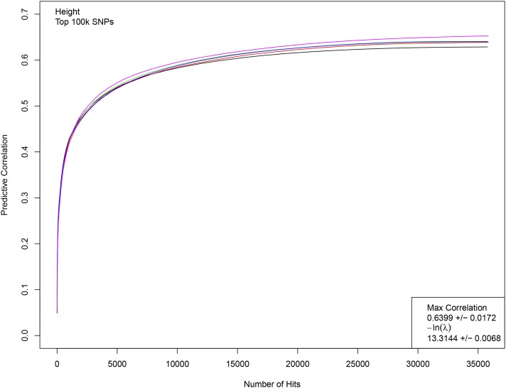
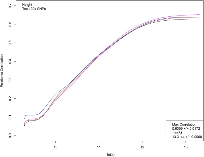
Figure 1 displays results from a typical LASSO run for height. Five nonoverlapping sets of 5k individuals each were held back from LASSO training using the top 100k candidate SNPs. For each value of the L₁ penalization λ, the resulting predictor ${\overrightarrow{\beta }}^{*}$ is applied to the genomes of the holdout sets and the correlation between predicted and actual height is computed. A phase transition (region of rapid variation in results) is expected and occurs at roughly $10<-\text{ln}\left(\mathit{\lambda }\right)<12.$ The penalization is reduced until the correlation is maximized. In Figure 1, the correlation is shown as a function of number of SNPs assigned nonzero effect sizes (i.e., activated) by LASSO. In the phase transition regime, where correlation rapidly increases, the number of activated SNPs grows rapidly from about zero to 7k. Each of the five colored curves in the figure corresponds to a training run on 453k individuals, with a different 5k held back (and slightly different training set) for each run. The phase transition is shown in terms of the penalization $-\text{ln}\left(\lambda \right)$ in Figure 2.

Figure 1.

Correlation between actual and predicted heights as a function of the number of SNP hits activated in the predictor. While difficult to visually separate, each line represents the training of a predictor using 453k individuals. Correlation is computed on five separate nonoverlapping sets of 5k individuals not used in training. The phase transition region (roughly, $10<-\text{ln}\left(\lambda \right)<12$) corresponds to rapid growth in correlation on this graph, with number of hits growing from near 0 to >5000. The correlation and penalization values given in the lower righthand corner are the average of a set of LASSO runs; each run generates a slightly different value (even, a slightly different beta vector).

Figure 2.

Correlation between actual and predicted heights as a function of L₁ penalization λ. Each line represents the training of a predictor using 453k individuals. Correlation is computed on 5k individuals not used in training. The correlation and penalization values given in the lower righthand corner are the average of a set of LASSO runs; each run generates a slightly different value (even, a slightly different beta vector).

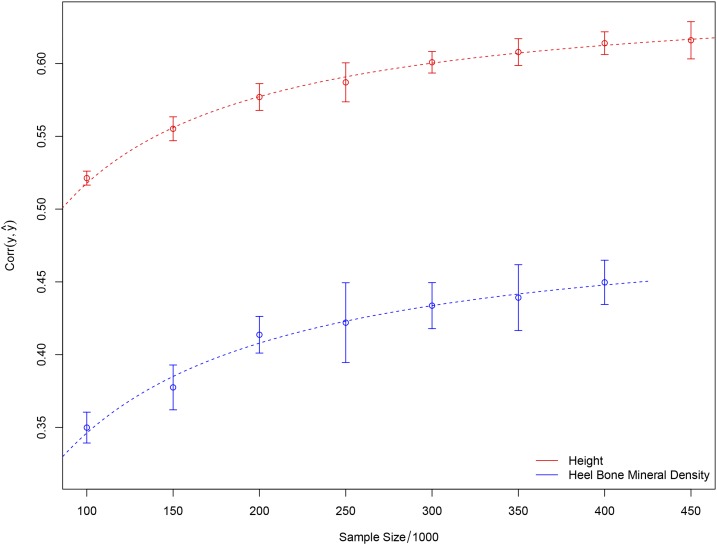
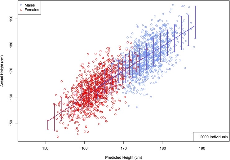
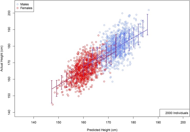
Figure 3 shows the correlation between predicted and actual phenotypes in a validation set of 5000 individuals not used in the training optimization described above—this is shown both for height and heel bone mineral density. The horizontal axis shows the number of individuals used in the training set, and the error bars reflect 1 SD uncertainty estimated from five replications. The correlation obtained indicates convergence to an asymptotic value of somewhat <0.7 (corresponding to roughly 50% of total variance) for height, and perhaps 0.45 for heel bone mineral density. Figure 4 shows a scatterplot (each point is an individual) of predicted and actual height for 2000 individuals (roughly equal numbers of males and females) not used in the training. The actual heights of most individuals are within ∼3 cm of the predicted value. In the LASSO training (see Appendix sections L₁-penalized regression and Coordinate Descent for more details) individuals are z-scored according to sex (i.e., relative to the M or F mean and SD), whereas in Figure 4 the actual (not z-scored) heights are shown for each individual. The correlation between predicted and actual heights in this figure is >0.7 because of differences between the two sexes. The predictor is equally accurate when applied to males or females (error bars are similar, as is correlation), once the z-scoring is inverted (i.e., using M/F means and SDs). We have checked this by running the predictor on all-male and all-female groups—specifically, a predictor generated using the top 100,000 SNPs achieved a maximum correlation $r=0.6526$ among the entire holdback set (both sexes) while the same predictor achieved correlations $r_M=0.6411$ and $r_F=0.6662$ among solely M/F groups in the holdback set.

Figure 3.

Correlation between predicted and actual height as number of individuals n in training set is varied. $p=50$k candidate SNPs used in optimization. Fit lines of the form $(\text{corr}.)\sim n/n+b$ are included to aid visualization.

Figure 4.

Actual height (centimeter) vs. predicted height (centimeter) using 2000 randomly selected individuals with a roughly even male–female ratio, held back from predictor training. Error bars indicate ± 1 SD range computed using larger validation set. (No corrections of actual height for age or gender were made; see Appendix L₁-penalized regression and Coordinate Descent for details of predictor training).

The corresponding result for EA does not indicate any approach to a limiting value. Using all the data in the sample, we obtain maximum correlation of ∼0.3, activating ∼10k SNPs. This compares favorably with results in Selzam et al. (2017). Presumably, significantly more or higher quality data will be required to capture most of the SNP heritability of this trait.

The number of activated SNPs in the optimal predictors for height and bone density is roughly 20k. Increasing the number of candidate SNPs used from $p=50$k to $p=100$k increased the maximum correlation of the predictors somewhat, but did not change the number of activated SNPs significantly.

Yang et al. (2010) provided the first GCTA estimates for the heritability of height $h_G^2\sim 0.45$—a result reproduced by others (Kim et al. 2017), and improved upon in more recent calculations: specifically, Rawlik et al. (2016) uses the UK Biobank and achieves $h_G^2\sim 0.53$ for height. There has been debate in the literature over the statistical properties of GREML (genome-wide restricted maximum likelihood) estimates of SNP heritability, and it is not clear that standard estimation methods yield reasonably unbiased estimates even with large sample size (Lee and Chow 2014; de los Campos et al. 2015; Gamazon and Park 2016; Kumar et al. 2015, 2016; Yang et al. 2016). It is possible (although we take no position on the question here) that GCTA estimates of SNP heritability should only be used as a rough guide, but these results suggest that for height $h_G^2\sim 0.45-0.55$ as a reasonable expectation. Independent of GCTA analyses, one can still determine a lower bound on the heritability of a trait over a specific set of genomic variants simply by building a predictor (Makowsky et al. 2011) to determine how much variance can be accounted for. The ability to predict based on genotype must have its basis in heritability, hence the lower bound.

For height we tested out-of-sample validity by building a predictor model using SNPs whose state is available for both UKBB individuals (via imputation) and on the Atherosclerosis Risk in Communities Study (ARIC 1989) individuals (the latter is a US sample). This SNP set differs from the one used above, and is somewhat more restricted due to the different genotyping arrays used by UKBB and ARIC. Training was done on UKBB data and out-of-sample validity tested on ARIC data. A ∼5% decrease in correlation results from the restriction of SNPs and limitations of imputation: the correlation fell to ∼0.58 (from 0.61) while testing within the UKBB. On ARIC participants, the correlation drops further by ∼7%, with a correlation of ∼0.54. Only this latter decrease in predictive power is really due to out-of-sample effects. It is plausible that if ARIC participants were genotyped on the same array as the UKBB training set, there would only be a ∼7% difference in predictor performance. An ARIC scatterplot analogous to Figure 4 is shown in the Appendix Out-of-sample validation. Most ARIC individuals have actual height within 4 cm or less of predicted height.

We also checked (see Appendix Confounding variables: age, sex, and family structure) that familial relationships in UKBB do not have an important impact on our results. LASSO training was done both on the full set of data and on a smaller data set where all first degree cousin or stronger relations were removed (kinship >0.10). After filtering for kinship on the calls, this left 423,510 individuals for height and 382,727 individuals for heel bone density. This unrelated dataset was used for model training using random sets of 100k, 150k, …, 400k individuals, and there was no discernible difference in the results between using a training set drawn from the set of 423,510 kinship-filtered individuals and individuals from the unfiltered set.

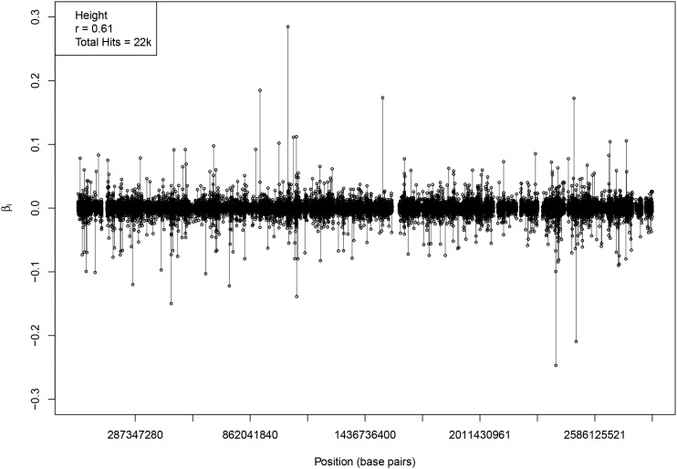
The genetic architecture of a height model is displayed in Figure 5, which shows the effect size (minor allele) and location of each activated SNP. The horizontal axis represents the SNP position in the genome, if each chromosome (1–22) were laid end to end to form a continuous linear region. The specific height predictor from which these SNPs are taken was built from 50k candidate SNPs and achieves a correlation between actual and predicted height of ∼0.61. The activated SNPs seem to be uniformly distributed across the genome.

Figure 5.

Effect size (minor allele) for each activated SNP in a predictor model. The horizontal axis represents the SNP position in the genome, if chromosomes (1–22) were connected end to end to form a continuous linear region. Activated SNPs are distributed roughly uniformly throughout the genome. The correlation value given in the upper lefthand corner is particular to a specific LASSO run. Each run generates a slightly different value (even, a slightly different beta vector). There are several gaps where no SNPs are activated – this is due to lack of coverage on the SNP array. For instance, the largest gap occurs on chromosome 9, where there exists a ∼18 million base-pair gap between SNPs (out of a total ∼138 million chromosome 9 base-pairs).

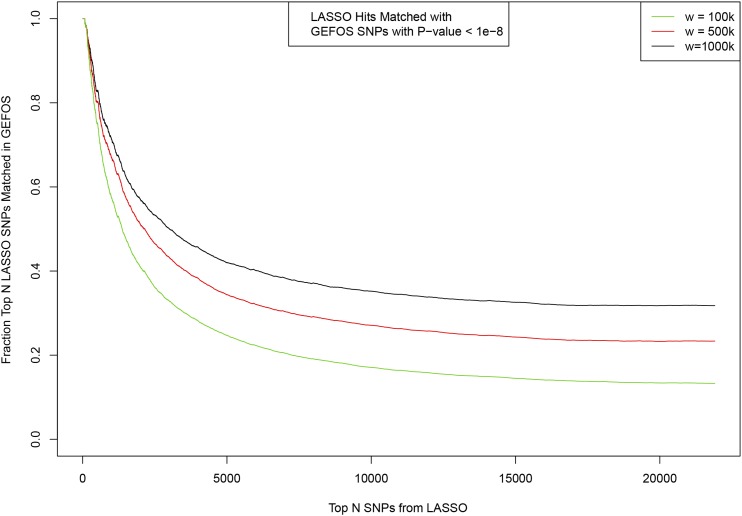
There is significant overlap between regions of the genome near previously known SNPs and regions identified by our algorithm (see Comparison to GWAS and LD between activated predictor SNPs and GIANT SNPs in the Appendix). Note, our activated SNPs are roughly uniformly distributed over the entire genome, and number in the many thousands for each trait. This means that many of our SNPs, including some of those that account for the most variance, are in regions not previously identified by earlier GWAS.

We explore the relationship of our results to GWAS results in more detail in sections Comparison to GWAS and LD between activated predictor SNPs and GIANT SNPs of the Appendix. As mentioned, it is possible in principle that some fraction of the SNPs activated in our predictor are actually false positives (i.e., are not actually associated with the trait). However, the overall statistical overlap between our activated SNPs and known GWAS loci is very high for the SNPs that account for the most variance in our predictor. For example, among the top 100 activated SNPs in our height predictor (ranked by variance accounted for), ∼85% are in direct LD (correlation) of 0.4 or higher with a genome-wide significant $\left(p<{10}^{-8}\right)$ GIANT 2014 SNP, and ∼90% are in LD (correlation) of 0.4 or higher with some combination of genome-wide significant GIANT 2014 SNPs. The typical correlation among ALL ∼20k activated LASSO SNPs to some best linear combination of GIANT 2014 SNPs is ∼0.4 (see figures in sections Comparison to GWAS and LD between activated predictor SNPs and GIANT SNPs of the Appendix.

Even those activated SNPs that are not in LD with known GIANT SNPs could be correlated to SNP(s) that fall below the GIANT genome-wide significance threshold, but nevertheless have an effect on height. In other words, due to the fact that not all height SNPs have been discovered by GIANT, it is not possible to conclude from the analysis described above that any specific activated SNP in our predictor is in fact a false positive. GIANT (Wood et al. 2014) identified $\sim 700$ variants clustered in 423 loci (not all of these are effectively independent variants), but this is probably only a fraction of all height associated variants. SNPs activated by LASSO might be correlated to linear combinations of SNPs below the $p<{10}^{-8}$ GIANT significance threshold, but which nevertheless contribute to total variance. Similarly, inclusion of more actual height variants into the GIANT set from which linear combinations are drawn could increase the max correlation to any given LASSO predictor SNP.

In any case, one can conclude that the vast majority of highly ranked predictor SNPs are linked to GIANT SNP(s) known to be associated with height.

We summarize average correlations achieved by predictors for various phenotypes in Table 1. Averages here are computed over five runs over mostly overlapping training sets; they differ by the previously mentioned 5k holdout sets. Additionally, when using a different SNP set, a new set of five runs is performed. For instance, after selecting imputed UKBB SNPs which overlap with ARIC SNPs (called from the array), a new set of LASSO predictors and correlation values was generated.

Table 1. A summary of the mean maximum correlation (and SD among runs) achieved between measured/predicted for each phenotype through LASSO.

Phenotype	SNP-set	SNPs used in LASSO	Test set	Prediction correlation (SE)
	UKBB calls	top-50k	UKBB	0.616 (0.013)
Height	UKBB calls	top-100k	UKBB	0.639 (0.017)
	UKBB imputed in common with ARIC	top-50k	UKBB	0.580
	UKBB imputed in common with ARIC	top-50k	ARIC	0.536
Heel bone density	UKBB calls	top-50k	UKBB	0.449 (0.015)
EA	UKBB calls	top-50k	UKBB	0.272 (0.022)

For height, LASSO runs were done using the top 50,000/,100,000 GWAS SNPs and also using a SNP set which overlaps with both the UKBB imputed SNPs and ARIC SNPs—this predictor was tested both in holdback sets from the UKBB and on the ARIC dataset (in and out of sample). EA, Educational attainment; UKBB UK Biobank; ARIC: Atherosclerosis Risk in Communities Study; LASSO: L1-penalized regression.

Finally, we compare our LASSO results to a more straightforward method that relies on single SNP linear regression followed by SNP selection to construct a predictor. (Earlier work using results from the GIANT 250k analysis achieved predictive variance ∼15% (Wood et al. 2014)). Using the same UKBB dataset, we first rank all SNPs (i.e., nonimputed SNPs that are directly called by the array) by P-value. We then select a subset of SNPs to use in the predictor as follows. (This is necessary because of the redundancy of correlated SNPs in many regions of the genome). Starting with the most significant SNP, we scan down the list by P-value, discarding any SNPs that are within a distance $w/2$ base-pairs of a SNP we have already chosen for the predictor. This produces a subset constructed from the most significant (by P-value) SNPs but with no two SNPs closer than $w/2$ in distance. When w is small, ∼100 kbp, this may result in >20k SNPs, in which case we keep only the top 20k. (This is to maintain consistency with our LASSO predictor, which typically activates ∼20k SNPs). Using these filtered subsets of SNPs, we build a predictors two different ways: (1) use the estimated effect sizes from single-marker regression (as used in Wood et al. 2014), and (2) perform a multi-marker ordinary least-squares (OLS) fit to determine effect sizes for each SNP (LASSO reduces to multi-marker OLS in the limit of zero penalization). The results are given in Table 2 below. The best predictors constructed in this manner achieve correlation ∼0.55, which is impressive, but significantly inferior to the LASSO predictors. This is not surprising, since LASSO does a more sophisticated optimization of which SNPs to activate in the construction of the predictor. Note that, while in agreement with the results presented in Wood et al. (2014), method (1) predictors (i.e., taking effects values from the single-marker regression) underperform compared with multi-marker OLS. This is because multi-marker OLS takes into account possible correlations between SNPs in different windows, whereas effect sizes estimated from single-marker regression does not. See Appendix Comparison to GWAS for a comparison of different methods, and a demonstration of LASSO preferring uncorrelated SNPs.

Table 2. Summary of the mean maximum correlation (and SD among runs) achieved between measured/predicted height using windowed predictors (windowed = select the most significant SNP among those in a region).

Window size (kbp)	List size	Number SNPs included	GWAS	OLS
1000	4,026 (4)	4,026 (4)	0.375 (0.007)	0.465 (0.009)
500	7,975 (9)	7,975 (9)	0.358 (0.010)	0.496 (0.010)
200	19,516 (14)	19,516 (14)	0.344 (0.010)	0.535 (0.006)
150	25,758 (21)	20,000	0.343 (0.010)	0.545 (0.010)
100	37,839 (14)	20,000	0.340 (0.012)	0.556 (0.012)
50	71,869 (40)	20,000	0.341 (0.010)	0.580 (0.009)

Correlations should be compared with LASSO results in Table A1. The two methods used are called GWAS (use effect sizes from single SNP regression results), and OLS (using multi-SNP regression on windowed SNPs). Note that, while in agreement with the results presented in Wood et al. (2014), GWAS underperforms compared with OLS since it does not take correlations between SNPs into account beyond windowing. SNP: Single nucleotide polymorphism; OLS ordinary least-squares; LASSO: L1-penalized regression; GWAS: genome-wide association studies.

Discussion

Until recently, most work with large genomic datasets has focused on finding associations between markers (e.g., SNPs) and phenotypes (Makowsky et al. 2011). In contrast, we focused on optimal prediction of phenotypes from available data. We show that much of the expected heritability from common SNPs can be captured, even for complex traits affected by thousands of variants. Recent studies using data from the interim release of the UKBB reported prediction correlations of ∼0.5 for human height using roughly 100k individuals in the training (Kim et al. 2017). These studies forecast further improvement of prediction accuracy with increased sample size, which we have confirmed here.

We are optimistic that, given enough data and high quality phenotypes, results similar to those for height might be obtained for other quantitative traits, such as cognitive ability or specific disease risk. There are numerous disease conditions with heritability in the 0.5 range, such as Alzheimer’s, type I diabetes, obesity, ovarian cancer, schizophrenia, etc. (SNPedia 2017). Even if the heritable risk for these conditions is controlled by thousands of genetic variants, our work suggests that effective predictors might be obtainable (i.e., comparable to the height predictor in Figure 4). This would allow identification of individuals at high risk from genotypes alone. The public health benefits are potentially enormous.

We can roughly estimate the amount of case-control data required to capture most of the variance in disease risk. For a quantitative trait (e.g., height) with $h^2\sim 0.5,$ our previous simulations (Vattikuti et al. 2014) predict that the phase transition in LASSO performance occurs at $n\sim 30s,$ where n is the number of individuals in the sample and s is the sparsity of the trait (i.e., number of variants with nonzero effect sizes). For case-control data, we find $n\sim 100s$ (where n means number of cases with equal number controls) is more than sufficient. Thus, using our methods, analysis of ∼100k cases together with a similar number of controls might allow good prediction of highly heritable disease risk, even if the genetic architecture is complex and depends on a 1000 or more genetic variants.

Appendix

Methods

UKBB dataset QC

In July 2017, the UK Biobank (Bycroft et al. 2017; UK Biobank 2017) released a set of 488,377 genotyped individuals that were genotyped using two Affymetrix platforms—∼50,000 samples on the UK BiLEVE Axiom array and the remainder on the UK Biobank Axiom array. The initial genotype information was collected for 488,377 individuals for 805,426 SNPs and then subsequently imputed. Quality Control was done on the unimputed data by: (1) removing SNPs which had missing call rates >3%, (2) removing individuals which had missing call rates >10%, and, so as not to deal with very rare variants, (3) removing SNPs which had minor frequencies <0.1%. The resulting genetic data contained 645,589 SNPs and 488,371 individuals. This set was then further filtered for self-reported Europeans (in the UKBB terminology, British, Irish, and Any Other White) for whom the necessary phenotype measurements were available: for height, the number of remaining individuals was 457,484; for heel bone mineral density there were 413,444 individuals; and for EA, there were 455,637 individuals. We performed additional training runs using only individuals who both self-identify as European ancestry and also are so identified using the top six PCA vectors from UKBB population structure. This reduced set includes 407,849 individuals, and the predictor results are very similar to the case of 400k self-identified Europeans. From this, we conclude that population stratification has a negligible effect on our predictor construction: specifically, using the procedure of setting aside a holdback set and selecting the top 50,000 SNPs we observe an average maximum correlation of $r=0.6273\left(0.0168\right)$ between holdback sets and genetic score.

As a further check of the effect of population stratification on prediction results, we tested to see whether we could account for a nontrivial proportion of variance using the top principal components of population structure. Using calls from the UKBB SNP array, we select $\sim$50,000 SNPs, which are roughly evenly separated on the genome and construct the top 10 principal component directions in SNP-space. This is done by constructing the LD matrix, $1/N{X}^{\prime }X,$, where N is the number of samples in a training set and $X_{ij}=\left(G_{ij}-{\mu }_j\right)/{\left(p_j\left(1-p_j\right)\right)}^{1/2}.$ Here, $G_{ij}$ is the genotype and $p_j$ are minor allele frequencies. We then project each individual in the training set onto the principal components and perform a multivariable OLS against height to obtain a predictor based on principal components of population structure, ${\beta }_{PC}.$ Amongst five separate validation sets, the predictor achieved a correlation of only $0.048\pm 0.024$ with height. This shows that any possible population stratification effects contribute a negligible amount to the total prediction accuracy.

The imputed data set was generated using the set of 805,426 raw markers using the Haplotype Reference Consortium and UK10K haplotype resources. After imputation and initial QC, there were a total of 92,060,613 SNPs and 487,411 individuals. From this imputed data, we further excluded SNPs and samples that had missing call rates of >3% and also removing SNPs with minor allele frequency (MAF) <0.1%. For out-of-sample validation of height, we extracted SNPs which survived the prior quality control measures, and are also present in a second (American) dataset from the Atherosclerosis Risk in Communities Study (ARIC 1989). This resulted in a total of 632,155 SNPs and 464,192 samples. All quality control steps, except for the imputation performed by the UK Biobank, were performed using version 1.9 of the Plink software (Chang et al. 2015).

Confounding variables: age, sex, and family structure

All traits for self-identified Europeans were adjusted on the basis of age and sex. The phenotypes for self-reported Europeans were adjusted by z-scoring the phenotypes amongst all individuals of the same sex. To correct for the effects of societal changes (“Flynn Effects”), a univariate linear regression was performed on z-scored phenotypes using year-of-birth as the dependent variable. The adjusted phenotype was set equal to the residual of the z-scored phenotype and the regression line. Before making these corrections, it was shown that the mean phenotypic value was indeed increasing with year-of-birth—this was seen in all three phenotypes: height, heel bone mineral density, and EA.

The adjustment parameters for the phenotypes are given in Table A.1. The phenotypes are first centered and scaled using the mean and SD for each sex (i.e., standardized), then the adjusted phenotype is fit to a linear function of year of birth (YOB) $y={\beta }_0+{\beta }_{\text{YOB}}\cdot \left(\text{YOB}\right)+\mathit{ϵ}$ When fitting based on year of birth, only cohorts between 1938 and 1968 were included, as the cohorts outside of this range were small in number. Finally, the linear trend was subtracted from the z-scored phenotypes to form the adjusted phenotype used in training of all models.

Relatedness calculations were provided with the UKBB dataset in order to account for family structure and cryptic relatedness. There were 107,163 familial relationships identified amongst UKBB participants which were at the level of third cousins or higher and, due to the large number of relationships, filtering out these individuals results in a nontrivial decrease in the size of data available for model selection. To investigate the relevance of this issue, LASSO training was done both on the full set of data and on a smaller data set where all first degree cousin or stronger relations were removed (kinship >0.10). After filtering for kinship on the calls, this left 423,510 individuals for height and 382,727 individuals for heel bone density. This unrelated dataset was used for model training using random sets of 100,000; 150,000 …, 400,000 individuals and there was no discernible difference in the results between using a training set drawn from the set of 423,510 kinship-filtered individuals and individuals from the unfiltered set. Therefore, we do not believe that the familial relationships have an important impact on our results.

L₁-penalized regression

Consider the regression problem in generality. We have n observations of the phenotype, $y_I,$ with $I=1,\dots ,n$ as the vector $\overrightarrow{y}.$ The genotype data are encoded in the $n\times p$ design matrix $X_{Ij}$ with $j=1,\dots ,p.$ Each entry $X_{Ij}$ is the number of copies of the most frequent minor allele of the jth SNP for the Ith person, and thus takes values 0, 1, or 2. After initial QC, missing values are mean-imputed.

We use a standard linear model for the dependence of y on the SNP data $x_j.$ That is, we assume a relationship of the form

$$y_I=y_0+\widehat{\overrightarrow{\beta }}\cdot {\overrightarrow{x}}_I+e_I,$$ (A1)

where the errors, $e_I,$ are assumed to be (identically and independent) normally distributed with unknown variance ${\sigma }_e.$ The errors, $e_I,$ receive contributions from potential environmental effects, gene–gene nonlinear effects, and gene–environment nonlinear effects. For discussion of methods to recover nonlinear effects, see Ho and Hsu (2015).

We compute an estimator ${\overrightarrow{\beta }}^{*}$ for the vector of linear effects, $\widehat{\overrightarrow{\beta }}\in {\mathrm{ℝ}}^p$, using L₁-penalized regression (LASSO) (Tibshirani 1996). This corresponds to minimizing the objective function (after standardizing $\overrightarrow{y}$ and X)

$${\overrightarrow{\beta }}^{*}=\underset{\overrightarrow{\beta }\in {\mathrm{ℝ}}^p}{\mathrm{argmin}}{O}_{\lambda }\left(\overrightarrow{y},X;\overrightarrow{\beta }\right),\hspace{1em}{O}_{\lambda }\left(\overrightarrow{y},X;\overrightarrow{\beta }\right)=\frac{1}{2}{\left|\left|\overrightarrow{y}-X\overrightarrow{\beta }\right|\right|}^2+n\lambda {\left|\right|\overrightarrow{\beta }\left|\right|}_1,$$ (A.2)

where λ is a penalty (hyper-)parameter and the L₁-norm is defined to be the sum of the absolute values of the coefficients

$${\left|\left|\overrightarrow{\beta }\right|\right|}_1={\displaystyle \sum _{j=1}^p\left|{\beta }_j\right|}.$$

(We use $\Vert \cdot \Vert$ with no subscript to denote the standard L₂-norm.) The extra factor of n in the second term is a convention that factors out the explicit sample size scaling of the penalization. The first term is the square of the L₂-norm of the residual.

The first term is the standard OLS loss function. The effect of the second term is to regularize the regression problem by favoring sparse solutions with the nonzero coefficients shrunk toward 0. This seems appropriate for genomic problems, since we expect that, for any given phenotype, most SNPs have no effect. Biasing the nonzero coefficients toward 0 reduces variance and improves the expected fit for small sample size.

Even for $n\ll p,$ LASSO can obtain an accurate $\overrightarrow{\beta }$ under the right conditions: the effects vector must be sparse and the heritability of the trait must be sufficiently high (equivalently, the amount of noise variance is bounded). For fixed ${\sigma }_e^2$ and sparse effects vector, there is a critical sample size $n^{*}$ (depending on ${\sigma }_e$ and the sparsity of the trait), above which one expects to get good recovery of $\overrightarrow{\beta }$ in terms of the L₂ error. A phase transition at $n\sim n^{*}$ has been demonstrated numerically for real and simulated genomic data in Vattikuti et al. (2014).

For our specific calculations, we use the following cross-validation procedure:

1. Break the data into training sets, and validation sets.

2. Perform a standard single-marker GWAS on the training sets only, and rank the SNPs by P-value.

3. To ease the computational burden, restrict the calculation to a fixed number of lowest P-value SNPs on each training set. Replace any missing SNP values by the SNP-mean for the training data.

4. Perform LASSO on the standardized training data, scanning a range of values for the penalty λ that passes through the phase transition region of rapid variation in results.

5. Choose the λ that has the maximum correlation on the validation set, which was held back from training.

6. Finally, evaluate performance of optimal predictor ${\beta }^{*}$ on out-of-sample test sets, when available.

Let us note that one could be concerned about reporting results on a validation set used to tune hyper-parameters; however, one expects any overtraining in fitting this single parameter to be insignificant. This is borne out by specific investigations of the authors using a second holdout set, and moreover by the model’s performance on out-of-sample test data not used in any previous step of the analysis.

Coordinate descent

Most algorithms for minimizing the objective function (A.2) use (some variation of) coordinate descent (Friedman et al. 2007, 2010).¹The basic form of the algorithm is as follows. Proceeding from an initial guess ${\overrightarrow{\beta }}_0,$ we cycle through the p “coordinates” sequentially, minimizing O with respect to each ${\beta }_j$ (holding others fixed). (Angle brackets denote sample averaging.) To that end, note that

$$\frac{\partial O}{\partial {\beta }_j}=n\left[\langle x_j^2\rangle {\beta }_j+{\displaystyle \sum _{k\ne j}\langle x_j{x}_k\rangle {\beta }_k-\langle x_{j}y\rangle +\mathit{\lambda }\text{sgn}\left({\beta }_j\right)}\right]=0.$$ (A.3)

Thus, the updated coefficient should satisfy

$${\beta }_j^{*}=\frac{1}{\langle x_j^2\rangle }\left[\langle x_{j}y\rangle -{\displaystyle \sum _{k\ne j}\langle x_j{x}_k\rangle {\beta }_k-\lambda \text{sgn}\left({\beta }_j^{*}\right)}\right].$$ (A.4)

To solve for ${\beta }_k^{*}$, one should determine the $\lambda =0$ solution. If it is positive (negative), then guess that $\text{sgn}\left({\beta }_j^{*}\right)$ should be positive (negative) and subtract (add) the λ term. If the sign flips, then the solution is spurious, and the optimal solution is at ${\beta }_j^{*}=0.$ (To see this, note that for ${\beta }_j^{*}=0^{+}$ the derivative is positive, and for ${\beta }_j^{*}=0^{-}$ the derivative is negative.)

Introduce the “soft thresholding function”

$$S\left(z,\gamma \right)=\text{sgn}\left(z\right)\max \left(\left|z\right|-\gamma ,0\right).$$ (A.5)

Then, the update for the jth component of $\overrightarrow{\beta }$ is

$${\beta }_j^{*}=\frac{1}{\langle x_j^2\rangle }S\left(\langle x_{j}y\rangle -{\displaystyle \sum _{k\ne j}\langle x_j{x}_k\rangle {\beta }_k,\lambda }\right).$$ (A.6)

The basic coordinate descent algorithm is as shown in Alg. 1.

Algorithm 1. Basic coordinate descent algorithm for LASSO:

Data.$X_{jI}$ and $y_I$ with $j=1,\dots ,p$ and $I=1,\dots ,n$.

Input. Penalty parameter λ, tolerance ϵ, and (optionally) initial guess ${\overrightarrow{\beta }}_0$.

Output. $\overrightarrow{\beta }$ solving LASSO optimization problem within convergence tolerance ϵ.

$$\overrightarrow{\beta }\leftarrow {\overrightarrow{\beta }}_0$$

repeat

$${\overrightarrow{\beta }}_0\leftarrow \overrightarrow{\beta }$$

for j in $\left\{1,\dots ,p\right\}$ do

$${\beta }_j\leftarrow \frac{1}{\langle x_j^2\rangle }S\left(\langle x_{j}y\rangle -{\displaystyle \sum _{k\ne j}\langle x_j{x}_k\rangle {\beta }_k,\lambda }\right)$$

end.

until. ${\left(\overrightarrow{\beta }-{\overrightarrow{\beta }}_0\right)}^2<{\mathit{ϵ}}^2$

return.$\overrightarrow{\beta }$

Out-of-sample validation

Model (i.e., predictor) construction was performed by implementing LASSO on the UK Biobank data. In order to validate models and check against overtraining, a second dataset is needed in order to test the results. We (1) withheld a small subset of UKBB individuals from the initial training for in-sample validation, and (2) applied the model to individuals from a completely different dataset (ARIC) for out-of-sample validation. In-sample validation was done by withholding a predetermined number of randomly selected individuals from the UK Biobank data before P-value cuts were applied to SNPs. The remaining individuals were used for LASSO training and the resulting model was applied to the individuals initially held back to check in-sample validity.

Out-of-sample validation is similar, except that we used a set of common SNPs for which values can be imputed on the UKBB individuals and are also known for ARIC individuals. Initial training of the model was performed using UKBB individuals, but its validity was then tested on the ARIC data. Results using the unimputed dataset reached correlation of ∼0.61 when testing within the UKBB. After selecting SNPs in common with ARIC, the correlation fell to ∼0.58 while testing within the UKBB, and achieved a correlation of ∼0.54 on ARIC participants. The ARIC results are shown in Figure A1 and Table 1. Actual heights of most individuals in the ARIC validation set are within 4 cm or less of the predicted height. We expect the performance loss from 0.58 to 0.54 can be explained by the different environments (which can couple to genetic variation) and different allele frequencies between the two populations.

The ARIC dataset (ARIC 1989) was composed of 12,772 Caucasian and African-American individuals who were genotyped on the Affymetrix 6.0 chip with 841,820 SNPs. This was filtered to keep only self-reported Caucasian individuals and SNPs with MAF >1% and missing call rates <5% with a final sample size of 9618 individuals with 705,956 SNPs. Filtering to only SNPs in common with the UKBB imputed data reduced the number of SNPs to 632,155.

Comparison to GWAS

We compare our activated predictor SNPs to known hits from GWAS collaborations studying the same phenotypes (Styrkarsdottir et al. 2008; Okbay et al. 2016; Marouli et al. 2017; Morris et al. 2017). Specifically we compare our results for height with those of the GIANT collaboration, for EA with SSGAC, and for Bone Density with GEFOS. We ordered activated SNPs (i.e., those assigned nonzero effect size β by the LASSO algorithm) by individual variance explained for a single SNP, $V_i,$

$$V_i=2\nu \left(1-\nu \right){\beta }_I^2,$$ (A.7)

where ν is the MAF. We then scanned down this list and looked for a proxy match by distance in the corresponding dataset.

For GIANT, we took the results published online (GIANT Consortium data files 2017) and extracted SNPs with $p<{10}^{-6}$ and $p<{10}^{-8}.$ When coarse grained into 1 Mbp regions, there were 423 independent loci with at least one SNP at $p<5\times {10}^{-8}.$

For SSGAC, we used the published results (Social Science Genetic Association Consortium: Data 2017) and kept SNPs with $p<{10}^{-6},$ a total of 316. These cluster in 74 independent regions.

For GEFOS (UKBB eBMD GWAS Data Release 2017 (GEFOS) 2017), we kept all SNPs with $p<{10}^{-8},$ which account for ∼20 regions.

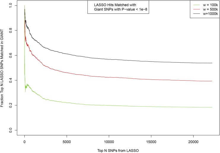
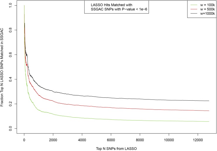
The results are displayed in Figures A.2, A.3, and A.4. They show significant overlap between regions of the genome near previously known SNPs and regions identified by our algorithm. However, our activated SNPs are roughly uniformly distributed over the entire genome, and number in the many thousands for each trait. This means that some of our SNPs, including some of those that account for the most variance, are in regions not previously identified by earlier GWAS. Again, these could be false positives. The top SNPs by variance in our predictors tend to overlap strongly with the loci (regions) identified in earlier GWAS.

As a further check of our predictors against earlier results, we select the top 100k SNPs ranked by P-value in the 2014 GIANT GWAS, almost all of which (>92%) have exact matches to imputed SNPs in UKBB data. We ran the LASSO algorithm on this specific SNP set using UKBB phenotype data, following our usual procedure (i.e., five runs with different 5000 individual holdout sets each time). This amounts to a test of our method specifically using (almost all of) the top GIANT SNPs. We obtain an average correlation between sex-age adjusted phenotype and predicted phenotype of 0.574 amongst the five different runs. (Each run has different training and holdback sets, and so returns slightly different predictor and resulting correlation. The average correlation that the resulting predictors achieve in the validation test is 0.574.) This slight reduction in correlation is due, at least in part, to imperfect imputation (we obtain the best results when using the calls on the array, with no imputation), which we observed before in our ARIC out-of-sample test. However, to compare with specific SNPs for which GIANT P-values are known we were forced to use imputed results.

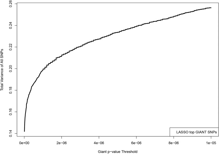
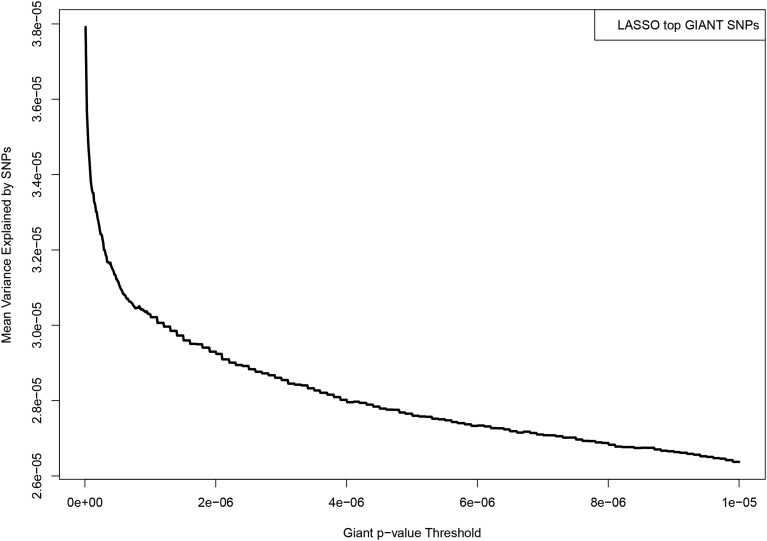
In Figure A5, we plot the fraction of total variance accounted for using Equation (A.7) (vertical axis) vs. SNP P-values according to the GIANT GWAS. We see that ∼80% of the total variance accounted by the predictor is due to SNPs with GIANT P-value below ${10}^{-6}.$ In Figure A6, we break the horizontal axis into 1000 equal bins (by P-value range), and plot the average variance accounted for the by SNPs in each bin. This distribution is strongly peaked, with lowest GIANT P-value SNPs accounting for much more variance on average than less GIANT significant SNPs. These graphs provide evidence that the LASSO predictor, when constructed by design from known GIANT SNPs, tends to utilize the most significant (by GIANT GWAS) SNPs to capture most of the predictive variance.

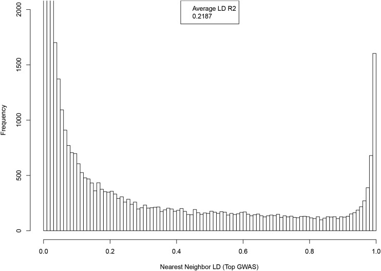
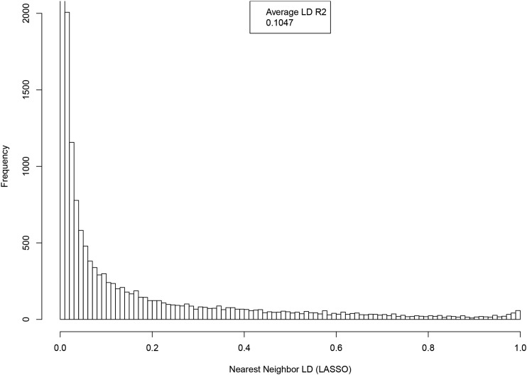
The LASSO algorithm favors sparsity: it only activates SNPs in the predictor when they increase its accuracy, net of the L₁ penalty. This leads to a set of activated SNPs that are relatively uncorrelated, since activating only one of a pair of highly correlated SNPs captures most of the predictive power from the pair without incurring the larger penalty that would come from activating both SNPs. This is illustrated in Figures A.7 and A.8, using height as the phenotype. The first, Figure A7, shows the distribution of LD $R^2$ between nearest neighbor SNPs (by location on the genome) among the top 50k SNPs ranked by P-value. The second, Figure A8, displays the LD distribution between nearest neighbors of SNPs activated in the predictor (i.e., selected by LASSO). As evident from the graphs, the GWAS SNPs include a nontrivial fraction of SNPs that are in high LD with their nearest neighbors, while this feature is absent in the LASSO results.

LD between activated predictor SNPs and GIANT SNPs

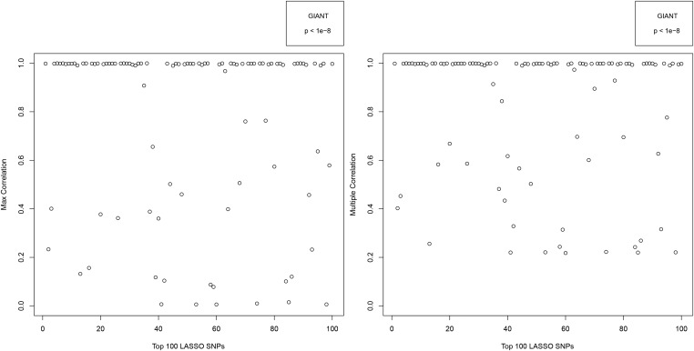
We analyzed the correlation between activated predictor SNPs (ranked by variance accounted for) and genome-wide significant $\left(p<{10}^{-8}\right)$ GIANT 2014 SNPs (henceforth, simply GIANT SNPs). For each activated predictor SNP, we computed two quantities: Max-Correlation (maximum correlation between the predictor SNP and any GIANT SNP) and Multi-Correlation (maximum correlation between the predictor SNP and any combination of GIANT SNPs). The Multi-Correlation statistic is computed using least squares optimization: for a given target SNP used in our predictor, we find the linear combination of GIANT SNPs that best predicts its state, and the Multi-Correlation statistic is simply this correlation.

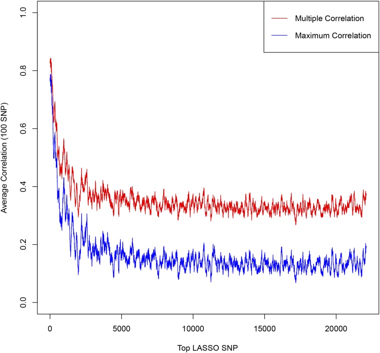
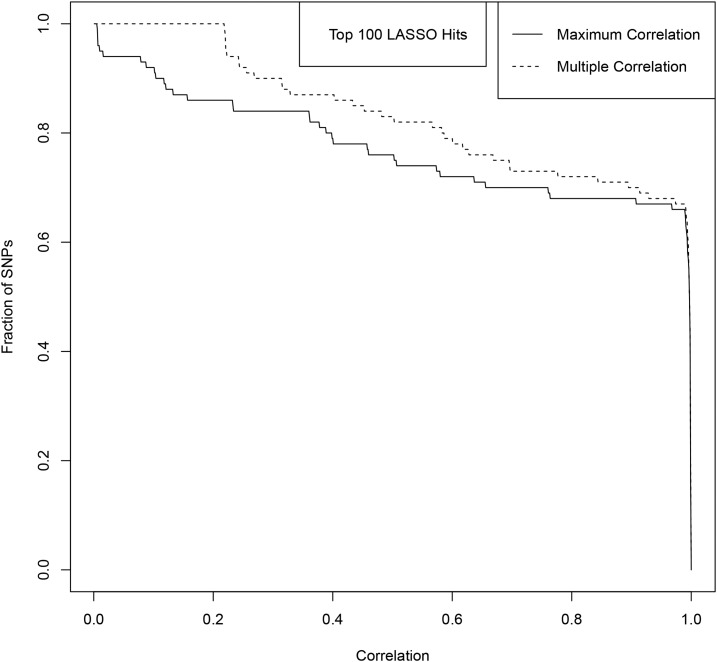
The results are shown in Figures A9–A13. Figures A9 and A11 shows the correlations for the top 100 LASSO SNPs while Figures A10, A12, and A13 show how the correlation with GIANT varies amongst the less significant LASSO SNPs.

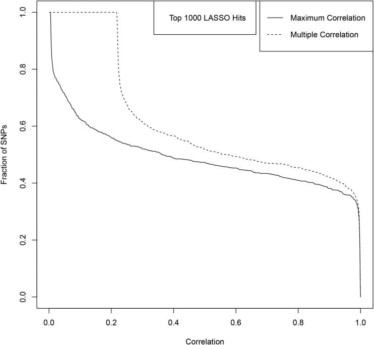
For example, among the top 100 activated SNPs in our height predictor (ranked by variance accounted for), ∼85% are in direct LD of 0.4 or higher with a genome-wide significant $\left(p<{10}^{-8}\right)$ GIANT 2014 SNP, and ∼90% are in LD of 0.4 or higher with some combination of genome-wide significant GIANT 2014 SNPs. Of the top 1000 activated SNPs in our predictor, ∼60% are in LD of 0.4 or higher with some combination of genome-wide significant GIANT 2014 SNPs.

Even those activated SNPs that are not in LD with known GIANT SNPs could be correlated to SNP(s) that fall below the GIANT genome-wide significance threshold, but nevertheless have an effect on height. In other words, due to the fact that not all height SNPs have been discovered by GIANT, it is not possible to conclude from the analysis described above that any specific activated SNP in our predictor is a false positive. GIANT (Wood et al. 2014) identified $\sim 700$ variants clustered in 423 loci (not all of these are effectively independent), but this is probably only a fraction of all height associated variants. SNPs activated by LASSO might be correlated to linear combinations of SNPs below the $p<{10}^{-8}$ GIANT significance threshold, but which nevertheless contribute to total variance. Similarly, inclusion of more actual height variants into the GIANT set from which linear combinations are drawn could increase the max correlation to any given LASSO predictor SNP.

In any case, one can conclude that the vast majority of highly ranked predictor SNPs are linked to GIANT SNP(s) known to be associated with height.

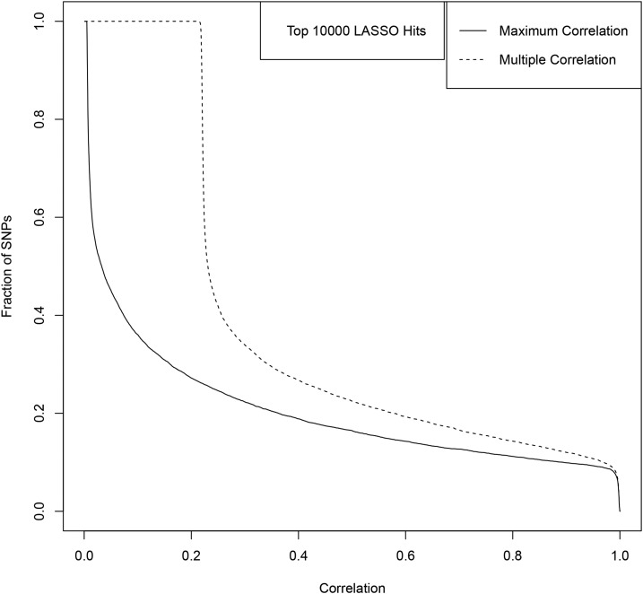
In Figures A.9, A.10, and A.13 we observe that the multiple correlation for any single LASSO SNP with GIANT SNPs has a nonzero minimum – i.e., the multiple correlation does not fall below ∼0.2 for any LASSO SNP. The multiple correlation floor can be understood in the context of regressing a dependent variable on a large number of independent variables. If all the regressor variables are independent, then the multiple correlation will be roughly equal to the L₂-norm of the individual correlations between the dependent variable and each regressor. One finds that each individual correlation scales as $1/\sqrt{n}$ with n being the number of samples. With p regressors, we expect the multiple correlation to scale as $\sqrt{p/n};$ this gives a nonzero baseline to the multiple correlation, explaining the qualitative behavior in the plots.

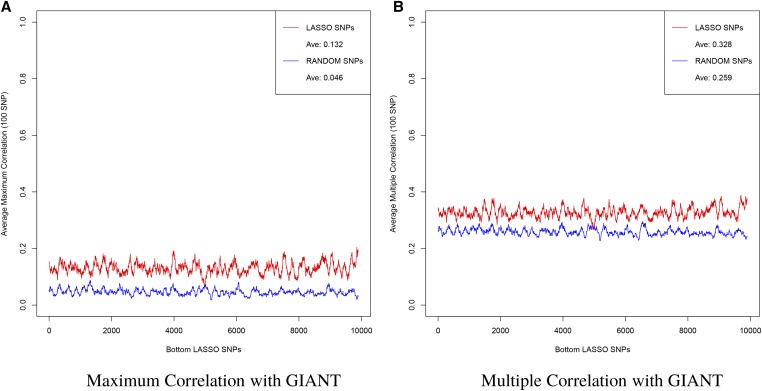
To answer the question of whether the LASSO SNPs are more correlated to the top GIANT SNPs than just randomly selected SNPs, we repeat the LD analysis with randomly selected SNPs. In Figure A14, we plot the rolling average of the maximum and multiple correlation of GIANT SNPs with the lowest ranked 10,000 LASSO SNPs and with 10,000 randomly selected SNPs. While the multiple correlation is low compared to the most significant LASSO hits (see Figure A10), we can see that even the least significant LASSO SNPs are more correlated to GIANT than what one would expect from random chance alone. The floor for multiple correlation of randomly selected SNPs with the 20,000 GIANT SNPs can be seen clearly in this plot. The gap between the LASSO and random SNPs signifies a level of correlation with GIANT better than random chance. It is important to note that the set of GIANT SNPs we refer to here have $p<{10}^{-8}.$ There are likely many more height-associated SNPs that do not reach this significance in GIANT. The elevated multiple correlation between our LASSO SNPs and the $p<{10}^{-8}$ GIANT SNPs is only partial indication of (i.e., lower bound on) their actual association with height.

Distribution of effect size sign

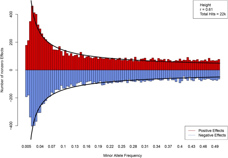
Figure A15 shows number of activated SNPs by sign of effect of the minor allele and MAF. The height of each bar represents the number of positive or negative effect SNPs in a MAF bin of width 0.005. The specific height predictor from which these SNPs are taken was built from 50k candidate SNPs and achieves a correlation between actual and predicted height of ∼0.61. The curves, which are meant to aid visualization, are constructed by fitting a power law $n\left(\nu \right)=a{\nu }^{-b}$ to the range $\nu \in \left(0.025,0.3\right)$ where ν is MAF and $n\left(\nu \right)$ is the number of nonzero effects. We exclude the smallest values of MAF because of incomplete discovery of SNPs in that region. The $\pm$ distributions are nearly symmetrical ($a_{+}=31.07,b_{+}=0.6553;$ $a_{-}=31.96;b_{-}=0.6404$), even at very small MAF. There does not appear to be a statistically significant deviation from random assignment of signs—the minor allele of an activated SNP is equally likely to increase or decrease height.

Figure A1.

Actual height (centimeter) vs. predicted height (centimeter) using 2000 randomly selected individuals (roughly equal numbers of males and females; no corrections for age or sex) from the ARIC dataset. Error bars indicate ± 1 SD range computed using larger validation set.

Figure A2.

Matching between top SNPs activated in predictor model ordered by variance accounted for (x-axis) and SNPs identified previously by GIANT 2014 GWAS (height). Fraction of the top LASSO SNPs which have a match in GIANT is shown on y-axis. Matching window size w given in base pair.

Figure A3.

Matching between top SNPs activated in predictor model ordered by variance accounted for (x-axis) and SNPs identified previously by SSGAC GWAS (EA). Fraction of the top LASSO SNPs which have a match in SSGAC is shown on y-axis. Matching window size w given in base pair.

Figure A4.

Matching between top SNPs activated in predictor model ordered by variance accounted for (x-axis) and SNPs identified previously by GEFOS GWAS (Heel Bone Density). Fraction of the top LASSO SNPs which have a match in GEFOS is shown on y-axis. Matching window size w given in base pair.

Figure A5.

The LASSO algorithm is used to construct a predictor from the most significant GIANT SNPs, nearly all of which can be found among UKBB imputed SNPs. Specifically, we took the top 50k SNPs which are in both the GIANT SNP set and the UKBB imputed SNP set, ordered by GIANT P-value. UKBB phenotypes are used as before. The specific predictor used for this graph achieves a correlation of 0.59 with height. The y-axis displays the fraction of the total variance accounted for by all activated LASSO SNPs with GIANT P-value less than that given on the x-axis. For example, if we take only GIANT SNPs with $p\mathrm{\lesssim }{10}^{-6}$ (in their analysis), and add up the individual variance accounted for by each SNP, we get $\sim \mathrm{0.2.}$ This is 80% of the total sum of individual variances accounted for by each activated SNP in the LASSO predictor.

Figure A6.

The LASSO algorithm is used to construct a predictor from the most significant GIANT SNPs, nearly all of which can be found among UKBB imputed SNPs. UKBB phenotypes are used as before. The specific predictor used for this graph achieves a correlation of 0.59. GIANT P-values of SNPs are displayed on the x-axis, and the average individual variance explained by SNPs within each of 1000 bins is computed and displayed on the y-axis.

Figure A7.

Distribution of LD $R^2$ between SNP and nearest neighbor (by location on genome), where both are the among the top 50k GWAS hits ranked by P-value.

Figure A8.

Distribution of LD $R^2$ between SNP and nearest neighbor (by location on genome), where both are activated in the LASSO predictor (22k).

Figure A9.

Maximum and Multiple Correlation with GIANT SNPS $\left(p<{10}^{-8}\right)$ for 100 top LASSO SNPs ranked by variance accounted for.

Figure A10.

Rolling average over 100 SNPs of Maximum/Multiple Correlation between LASSO and GIANT SNPs.

Figure A11.

The fraction of top 100 LASSO SNPs (ranked by variance) with Maximum/Multiple Correlation to GIANT SNPs $\left(p<{10}^{-8}\right)$ above a threshold given by the by the x-axis value. The solid line represents Maximum Correlation and the dashed line represents the Multiple Correlation.

Figure A12.

The fraction of top 1000 LASSO SNPs (ranked by variance) with Maximum/Multiple Correlation to GIANT SNPs $\left(p<{10}^{-8}\right)$ above a threshold given by the x-axis value. The solid line represents Maximum Correlation and the dashed line represents the Multiple Correlation.

Figure A13.

The fraction of top 10,000 LASSO SNPs (ranked by variance) with Maximum/Multiple Correlation to GIANT SNPs $\left(p<{10}^{-8}\right)$ above a threshold given by the x-axis value. The solid line represents Maximum Correlation and the dashed line represents the Multiple Correlation.

Figure A14.

The (A) Maximum and (B) Multiple Correlation between GIANT SNPs with the bottom 10,000 LASSO SNPs and 10,000 SNPs selected at random computed as a rolling average over 100 SNPs. Note that in both cases the least significant LASSO SNPs show a tighter correlation than randomly selected SNPs.

Figure A15.

Number of SNPs with positive (red) and negative (blue) minor allele effect sizes. Curves are constructed by fitting a power law in MAF. The correlation value given in the upper righthand corner is particular to a specific LASSO run; each run generates a slightly different value (even, a slightly different beta vector).

Table A1. Parameters used to z-score phenotypes and adjust for birth year $\left({\beta }_0,{\beta }_{\text{YOB}}\right)$.

	Height (cm)	Heel bone density $\left(g/c{m}^2\right)$)	Education (years)
Mean (male)	175.8	0.57	15.3
Mean (female)	162.7	0.51	14.6
SD (male)	6.77	0.15	5.13
SD (female)	6.12	0.12	5.08
Intercept $\left({\beta }_0\right)$	−47.1	−30.8	−55.6
Slope $\left({\beta }_{\text{YOB}}\right)$	0.024	0.016	0.028

Literature Cited

- ARIC , 1989. The decline of ischaemic heart disease mortality in the ARIC study communities. The ARIC Study Investigators”. Int. J. Epidemiol. 18(3 Suppl. 1): 88–98. [DOI] [PubMed] [Google Scholar]
- Bezanson J., Karpinski S., Shah V. B., Edelman A., 2012. Julia: a fast dynamic language for technical computing. arXiv :1209.5145.
- Bycroft C., Freeman C., Petkova D., Band G., Elliott L. T., et al. , 2017. Genome-wide genetic data on 500, 000 UK Biobank participants. BioRxiv: 166298 10.1101/166298 [DOI] [Google Scholar]
- Chang C. C., Chow C. C., Tellier L. C., Vattikuti S., Purcell S. M., et al. , 2015. Second-generation PLINK: rising to the challenge of larger and richer datasets. GigaScience 4: 7 10.1186/s13742-015-0047-8 [DOI] [PMC free article] [PubMed] [Google Scholar]
- de los Campos G., Gianola D., Allison D. B., 2010. Predicting genetic predisposition in humans: the promise of whole-genome markers. Nat. Rev. Genet. 11: 880–886. 10.1038/nrg2898 [DOI] [PubMed] [Google Scholar]
- de los Campos G., Sorensen D., Gianola D., 2015. Genomic heritability: what is it∼ PLoS Genet. 11: e1005048 10.1371/journal.pgen.1005048 [DOI] [PMC free article] [PubMed] [Google Scholar]
- El Ghaoui L., Viallon V., Rabbani R., 2012. Safe feature elimination in sparse supervised learning. Pac. J. Optim. 8: 667–698. [Google Scholar]
- Fercoq O., Gramfort A., Salmon J., 2015. Mind the duality gap: safer rules for the Lasso. arXiv :1505.03410.
- Friedman J., Hastie T., Höfling H., Tibshirani R., 2007. Pathwise coordinate optimization. Ann. Appl. Stat. 1: 302–332. 10.1214/07-AOAS131 [DOI] [Google Scholar]
- Friedman J., Hastie T., Tibshirani R., 2010. Regularization paths for generalized linear models via coordinate descent. J. Stat. Softw. 33: 1–22. 10.18637/jss.v033.i01 [DOI] [PMC free article] [PubMed] [Google Scholar]
- Gamazon E. R., Park D. S., 2016. SNP-based heritability estimation: measurement noise, population stratification, and stability. BioRxiv: 040055 10.1101/040055 [DOI]
- GIANT Consortium data files , 2017. Available at: https://portals.broadinstitute.org/collaboration/giant/index.php/GIANT_consortium_data_files.
- Ho C. M., Hsu S. D., 2015. Determination of nonlinear genetic architecture using compressed sensing. GigaScience 4: 44 10.1186/s13742-015-0081-6 [DOI] [PMC free article] [PubMed] [Google Scholar]
- Kim H., Grueneberg A., Vazquez A. I., Hsu S., de los Campos G., 2017. Will big data close the missing heritability gap∼ Genetics 207: 1135–1145. 10.1534/genetics.117.300271 [DOI] [PMC free article] [PubMed] [Google Scholar]
- Krishna Kumar, S., M. W. Feldman, D. H. Rehkopf, and S. Tuljapurkar, 2016 Limitations of GCTA as a solution to the missing heritability problem. Proc. Natl. Acad. Sci. USA. 113: E61–E70 (erratum: Proc. Natl. Acad. Sci. USA. 113: E813) [DOI] [PMC free article] [PubMed] [Google Scholar]
- Kumar S. K., Feldman M. W., Rehkopf D. H., Tuljapurkar S., 2016. Response to commentary on “limitations of GCTA as a solution to the missing heritability problem”. BioRxiv: 039594 10.1101/039594 [DOI] [PMC free article] [PubMed] [Google Scholar]
- Lee, J. J., C. C., Chow, 2014. Conditions for the validity of SNP-based heritability estimation. Hum. Genet. 133: 1011–1022. 10.1007/s00439-014-1441-5 [DOI] [PMC free article] [PubMed] [Google Scholar]
- Liu, J., Z. Zhao, J. Wang, and J. Ye, 2014 Safe screening with variational inequalities and its application to Lasso, pp. 289–297 in Proceedings of The 31st International Conference on Machine Learning, edited by Eric P. Xing and Tony Jebara. Vol. 32. 1. JMLR Workshop and Conference Proceedings. Brookline, MA: Microtome Publishing. [Google Scholar]
- Makowsky R., Pajewski N. M., Klimentidis Y. C., Vazquez A. I., Duarte C. W., et al. , 2011. Beyond missing heritability: prediction of complex traits. PLoS Genet. 7: e1002051 10.1371/journal.pgen.1002051 [DOI] [PMC free article] [PubMed] [Google Scholar]
- Malti, A., and C. Herzet, 2016 Safe screening tests for LASSO based on firmly non-expansiveness. 2016 IEEE International Conference on Acoustics, Speech and Signal Processing (ICASSP). New York: IEEE. [DOI] [Google Scholar]
- Marouli E., Graff M., Medina-Gomez C., Lo K. S., Wood A. R., et al. , 2017. Rare and low-frequency coding variants alter human adult height. Nature 542: 186–190. 10.1038/nature21039 [DOI] [PMC free article] [PubMed] [Google Scholar]
- Morris J. A., Kemp J. P., Medina-Gomez C., Forgetta V., Warrington N. M., et al. , 2017. Genome-wide association study of Heel Bone mineral density identifies 153 novel Loci and implicates functional involvement of GPC6 in osteoporosis. Nature Genetics 49: 1468–1475. [DOI] [PMC free article] [PubMed] [Google Scholar]
- Okbay A., Beauchamp J. P., Fontana M. A., Lee J. J., Pers T. H., et al. , 2016. Genome-wide association study identifies 74 loci associated with educational attainment. Nature 533: 539–542. 10.1038/nature17671 [DOI] [PMC free article] [PubMed] [Google Scholar]
- Rawlik K., Canela-Xandri O., Tenesa A., 2016. Evidence for sex-specific genetic architectures across a spectrum of human complex traits. Genome Biol. 17: 166 10.1186/s13059-016-1025-x [DOI] [PMC free article] [PubMed] [Google Scholar]
- Selzam, S., E. Krapohl, S. von Stumm, P. F. O’Reilly, K. Rimfeld et al., 2017 Predicting educational achievement from DNA. Mol. Psychiatry 22: 267–272 [corrigenda: Mol. Psychiatry 23: 161 (2018)] [DOI] [PMC free article] [PubMed] [Google Scholar]
- SNPedia , 2017. Available at: https://www.snpedia.com/index.php/Heritability
- Social Science Genetic Association Consortium: Data , 2017. Available at: https://www.thessgac.org/data.
- Styrkarsdottir U., Halldorsson B. V., Gretarsdottir S., Gudbjartsson D. F., Walters G. B., et al. , 2008. Multiple genetic loci for bone mineral density and fractures. N. Engl. J. Med. 358: 2355–2365. 10.1056/NEJMoa0801197 [DOI] [PubMed] [Google Scholar]
- Tibshirani R., 1996. Regression shrinkage and selection via the Lasso. J. R. Stat. Soc. B 58: 267–288. [Google Scholar]
- UKBB eBMD GWAS Data Release 2017 (GEFOS) , 2017. Available at: http://www.gefos.org/∼q=content/ukbb-ebmd-gwas-data-release-2017.
- UK Biobank, 2017 Available at: http://www.ukbiobank.ac.uk/. Accessed: July 21, 2017.
- Vattikuti S., Lee J. J., Chang C. C., Hsu S. D. H., Chow C. C., 2014. Applying compressed sensing to genome-wide association studies. GigaScience 3: 10 10.1186/2047-217X-3-10 [DOI] [PMC free article] [PubMed] [Google Scholar]
- Visscher P. M., Wray N. R., Zhang Q., Sklar P., McCarthy M. I., et al. , 2017. 10 years of GWAS discovery: biology, function, and translation. Am. J. Hum. Genet. 101: 5–22. 10.1016/j.ajhg.2017.06.005 [DOI] [PMC free article] [PubMed] [Google Scholar]
- Wood A. R., Esko T., Yang J., Vedantam S., Pers T. H., et al. , 2014. Defining the role of common variation in the genomic and biological architecture of adult human height. Nat. Genet. 46: 1173–1186. 10.1038/ng.3097 [DOI] [PMC free article] [PubMed] [Google Scholar]
- Yang J., Benyamin B., McEvoy B. P., Gordon S., Henders A. K., et al. , 2010. Common SNPs explain a large proportion of the heritability for human height. Nat. Genet. 42: 565–569. 10.1038/ng.608 [DOI] [PMC free article] [PubMed] [Google Scholar]
- Yang J., Lee S. H., Goddard M. E., Visscher P. M., 2011. GCTA: a tool for genome-wide complex trait analysis. Am. J. Hum. Genet. 88: 76–82. 10.1016/j.ajhg.2010.11.011 [DOI] [PMC free article] [PubMed] [Google Scholar]
- Yang J., Lee S. H., Wray N. R., Goddard M. E., Visscher P. M., 2016. GCTA-GREML accounts for linkage disequilibrium when estimating genetic variance from genomewide SNPs. Proc. Natl. Acad. Sci. USA. 113: E4579–E4580. 10.1073/pnas.1602743113 [DOI] [PMC free article] [PubMed] [Google Scholar]
Associated Data
This section collects any data citations, data availability statements, or supplementary materials included in this article.
Data Availability Statement