MRI‐based, wireless determination of the transfer function of a linear implant: Introduction of the transfer matrix

Abstract

Purpose

We introduce the transfer matrix (TM) that makes MR‐based wireless determination of transfer functions (TFs) possible. TFs are implant specific measures for RF‐safety assessment of linear implants. The TF relates an incident tangential electric field on an implant to a scattered electric field at its tip that generally governs local heating. The TM extends this concept and relates an incident tangential electric field to a current distribution in the implant therewith characterizing the RF response along the entire implant. The TM is exploited to measure TFs with MRI without hardware alterations.

Theory and Methods

A model of rightward and leftward propagating attenuated waves undergoing multiple reflections is used to derive an analytical expression for the TM. This allows parameterization of the TM of generic implants, e.g., (partially) insulated single wires, in a homogeneous medium in a few unknowns that simultaneously describe the TF. These unknowns can be determined with MRI making it possible to measure the TM and, therefore, also the TF.

Results

The TM is able to predict an induced current due to an incident electric field and can be accurately parameterized with a limited number of unknowns. Using this description the TF is determined accurately (with a Pearson correlation coefficient R ≥ 0.9 between measurements and simulations) from MRI acquisitions.

Conclusion

The TM enables measuring of TFs with MRI of the tested generic implant models. The MR‐based method does not need hardware alterations and is wireless hence making TF determination in more realistic scenarios conceivable.

1. INTRODUCTION

An ever‐growing part of the population is carrying active implanted medical devices (AIMDs). These people are often not eligible for MRI investigations because the scanner interacts with the AIMD through its electromagnetic fields potentially resulting in harm to the patient. The most pressing concern is that the AIMD may be able to locally enhance the RF fields of the MRI scanner. This can cause a local temperature hotspot with possibly severe consequences.1 Many factors influence the extent of the heating2, 3, 4, 5, 6 making it difficult to predict the occurrence of hazardous situations. This leads to many implants being considered a contraindication for MRI. Withholding these patients from such a diagnostically powerful image modality is unfortunate and hence RF heating is a topic of ongoing research. Likewise, implant manufacturers develop more and more products that can be used safely in an MRI‐scanner provided exposure conditions specified in a conditional label are met.

For this purpose, a technical specification7 has been formulated that provides a consistent testing methodology for implant manufacturers on how to assess the RF safety of implantable medical devices under MRI conditions. A four‐tier approach is described in this technical specification. The highest (fourth) tier performs the analysis with lowest amount of assumptions or simplifications allowing minimization of the overestimation of safety margins on relevant MR parameters such as for example the specific absorption rate (SAR). The cost is, however, an enormous set of numerically expensive simulations comprised of a vast selection of realistic implant positions in numerous human models to build a statistical basis for a prediction of an expected worst case heating. It involves accurate modeling of the often submillimeter details of the implant in a comparatively large volume of an MRI body coil. This combination will in many cases lead to prohibitive calculation times and/or extensive computational power.

The other tiers make use of the transfer function (TF) concept of the implant8 and rely on the usually localized nature of heating. The normalized TF is an implant characteristic that relates an incident tangential electric field distribution along the trajectory of a linear implant to the resultant, enhanced electric field (often around the tip) of the implant, which drives local heating. In fact the most significant field enhancement does not necessarily occur at the tip. The active implantable medical devices considered in this study typically contain an insulated wire having one or more electrode poles in contact with human tissue to deliver therapeutic currents. RF currents can be induced on these conductive structures during an MRI exam that result in energy deposition nearby these poles. Because the poles are most often located near the tip of these implants, this type of heating is often referred to as tip heating. In this work we used linear, (partially) insulated structures as a surrogate model that are characterized by similar RF current induction and also demonstrate tip heating. The TF simplifies computations because it decouples the assessment of the local scattered field (requiring detailed modeling of an implant) from the incident field (a characteristic of the comparatively large MRI system).

This function can be determined by monitoring the response of an implant to piece wise, localized electric field exposures with dedicated bench setups.9 Recently, based on the principle of reciprocity an alternative approach has been presented that interchanges the exposure and monitoring locations.10 This finding triggered the idea of MR‐based TF determination.11 For this method, a coax cable is soldered to the implant, which is used as a transmit/receive antenna in a phantom during MRI experiments. From the resulting images, the current distribution along the implant is determined that directly reflects the TF. This MR‐based methodology has the advantage that the TF can be determined without dedicated bench setups. The required galvanic contact, however, limits the practical applicability of the method and potentially perturbs the TF of the implant.

To avoid this physical alteration to the implant this study aims to use a regular MRI RF transmission technique (i.e., using the birdcage body coil for transmit). When E‐fields arising from the birdcage body coil impinge upon an implant, they excite a current that can be measured by an MRI experiment. This, effectively, enables the determination of the TF of the implant. However, contrarily to other experimental methods9, 10, 11 the resulting E‐field excitation is not localized at the tip and, therefore, the induced current distribution will not directly reflect the TF. Nevertheless, the TF (or its generalization, i.e., the transfer matrix [TM] introduced here) describing the current induction in an implant due to a tangential electric field, can be derived from the combined information contained in the incident E‐field and the induced current.

This work will show how a standard MRI measurement is also able to provide the TF for an implant‐like structure in a standardized test phantom. For this purpose, we will use a description that is a generalization of the TF. This extension, called the TM, relates an incident electric field distribution along the implant to the resultant current distribution over the entire implant instead of a single point. This generalization is necessary because the body coil excites the implant over the entire length and the excitation is not confined to the tip of the implant anymore as was originally assumed in the reciprocal approach for TF determination.10 With the assessment of the TM, the TF is simultaneously determined A test setup with known properties has to be used as this enables the determination of the incident electric field by means of electromagnetic simulations.

The TM can be determined through a Greens function approach by application of localized excitation at a range of positions along the implant and measurement of the current distribution along the implant for each excitation position. This is possible in simulations, but is not feasible in an MRI setting. In fact, normally only one incident E‐field distribution can be applied and only one current distribution along the wire can be measured. However, it will be shown for implant‐like structures that the TM can be parameterized by an analytical model, depending only on a few unknowns (∼6–10 unknowns for the cases considered in this work) that determine the entire matrix. The parameterization is derived for bare and (partially) insulated wires embedded in a homogenous dielectric. The application of this model provides a drastic reduction of the number of unknowns in the TM making it possible to determine it with conventional MRI measurements.

First, this parameterization of the TM will be derived in the theory section based on a model of converging sums of attenuated back and forth reflected waves. Second, the theoretical description will be validated with simulation results. After this, the feasibility of measuring the TM with MRI‐measurable quantities is demonstrated by extracting these quantities from simulations. Lastly, the actual MRI‐based TM assessment is demonstrated experimentally for two generic structures similar to ones used when the TF was first introduced in the context of RF safety.8 It should be noted that these generic structures do not resemble any realistic implant that are often much more complex. However, for a proof of principle of the method presented here, these generic structures suffice. The result is an MRI method that can assess the TF of a medical implant in a standardized phantom without the need for a galvanic contact to the implant.

2. THEORY

2.1. A simplified model

We will start with a theoretical treatise of a one‐dimensional implant model. It is composed of a single metallic wire of length $L$ embedded in a homogenous, lossy dielectric. If the implant is exposed to a localized, discretized RF electric field, a propagating, electromagnetic wave along the implant will be induced.

If the electric excitation incident at the tip of the implant, i.e., at $z=0$ behaves as an infinitesimal field source the current distribution in the wire will reflect the TF.10 An example of such a current distribution for a partially insulated wire is shown in Figure 1. This “tip excitation” will initially create an electromagnetic wave resulting in a current of magnitude ${\sigma }_{eff}A{E}_0$ that propagates toward the opposite end of the wire at $z=L$ and subsequently will reflect leftward. At $z=0$ it will be reflected in the opposite direction again. The complex reflection coefficients at the ends of the wire at $z=0$ and $z=L$ will be called ${\Gamma }_0$ and ${\Gamma }_L$, respectively. This repetitive process results in ever smaller wave amplitudes due to attenuation upon propagation through the implant. The sum of these waves is given by,

$$I\left(z\right)={\sigma }_{eff}A{E}_0(e^{-c_{1}z}+{\Gamma }_L{e}^{-c_{1}L}{e}^{c_1\left(z-L\right)})\left(1+{\Gamma }_0{\Gamma }_L{e}^{-2c_{1}L}+{\left({\Gamma }_0{\Gamma }_L{e}^{-2c_{1}L}\right)}^2+\dots \right).$$ (1)

Figure 1.

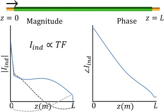
The real part of the first induced and reflected wave due to an excitation at the tip of the implant are shown as dashed lines in the left plot. The sum of these waves converges to the transfer function (TF) of which the magnitude (left) and phase (right) are shown as solid blue lines. They are the first column of the transfer matrix, M

Here $c_1$ is the complex wave number that describes the propagation of the electromagnetic wave through the implant. A is a proportionality factor with the dimension of a surface determined by the effective cross‐sectional area of the implant. ${\sigma }_{eff}$ is the effective conductivity that is governed by local loading conditions of the implant and relates the incident electric field, $E_0$, to an induced current. The geometric series in this equation bears similarities with summations often used in the field of optics.12 It converges to ${\left(1-{\Gamma }_0{\Gamma }_L{e}^{-2c_{1}L}\right)}^{-1}$.13 The resultant function is a standing wave that parameterizes the TF of an implant in the aforementioned four complex unknowns, i.e., the wave number $c_1$, the effective conductivity ${\sigma }_{eff}$ and the two reflection coefficients ${\Gamma }_0$ and ${\Gamma }_L$. For a detailed derivation of Equation (1) the reader is referred to the Supporting Information. Figure S1 in the Supporting Information, which is available online, displays the first view waves of the geometric series.

Note that $c_1$ and ${\sigma }_{eff}$ are complex constants as long as the implant is embedded in a homogeneous medium. If the electromagnetic properties of the environment around the implant vary along its length these quantities will be position dependent. This will increase the complexity of the model and not be addressed here. These two parameters as well as ${\Gamma }_0$ and ${\Gamma }_L$ will be dependent on the characteristics of the implant and on the electromagnetic properties of its environment. For more complicated structures a similar analysis will yield comparable equations with additional unknowns. The accuracy of this model to represent TFs will be demonstrated in the results section.

However, in this work we aim to extend the concept of the one‐dimensional TF toward a two‐dimensional TM, which is required to measure the TF with MRI experiments. This extension is necessary because during an MRI exam the incident electric field is not confined to the tip of an implant but distributed along its entire length. In this situation each position on the implants becomes a source for induced currents. The net induced current is the superposition of all these individual induced currents and can be described by the multiplication of the TM and the tangential, incident electric field vector. Therefore, we assume that the excitation does not occur at the tip of the implant, i.e., at $z=0$, but at some arbitrary location $z=z_j$. It will have a complex value $E\left(z_j\right)$. For all practical purposes this excitation will have a certain finite width, that will determine the resolution in which the TM and TF are rendered. The derivation of the TM will be continued in this discretized space. The excitation will create both a rightward and a leftward propagating (primary) electromagnetic wave with respect to the excitation that induces currents described by,

$$I_p\left(z_i,z_j\right)={\sigma }_{eff}AE\left(z_j\right)e^{-c_1\left|z_i-z_j\right|}.$$ (2)

These primary (i.e., primary in this case indicates a wave that is not reflected) rightward and a leftward propagating waves will again be repeatedly reflected at either end of the implant. The total sum of waves will be (see Supporting Information. for the details on this derivation):

$$\begin{array}{l}M\left(z_i,z_j\right)=I_p/E\left(z_j\right)+\frac{{\sigma }_{eff}A}{1-{\Gamma }_0 {\Gamma }_L{e}^{-2c_{1}L} }(\sqrt{{\Gamma }_0{\Gamma }_L{e}^{-2c_{1}L}}\text{cosh}(c_1\left(z_i+z_j-L\right)-\frac{1}{2}\text{ln}\left(\frac{{\mathrm{\Gamma }}_0}{{\mathrm{\Gamma }}_L}\right))+{\mathrm{\Gamma }}_0{\mathrm{\Gamma }}_L{e}^{-2c_{1}L}\text{cosh}\left(c_1\left(z_i-z_j\right)\right).\end{array}$$ (3)

This two‐dimensional function when multiplied with an electric field distribution incident on a wire gives the current distribution along this wire. For three different excitation positions the induced currents are shown in Figure 2.

Figure 2.

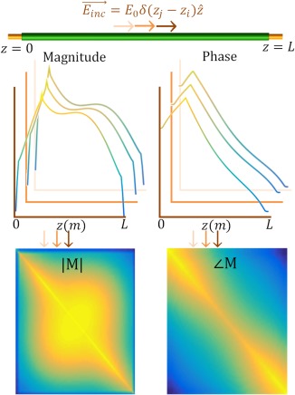
Excitations at various locations along the implant induce various current distributions. Three examples are shown as solid colored lines. These current distributions form the columns of the transfer matrix, M. The TF is the first column of the transfer matrix10

If an incident electric field distribution is known up to a certain resolution along the length of the implant, $E_{inc}\left(z_j\right)$, the resultant induced current distribution throughout the implant is computed through a simple matrix vector multiplication, $I_{ind}\left(z_i\right)=M\left(z_i,z_j\right)E_{inc}\left(z_j\right)$. The TM describes the RF response of an implant to an electric field exposure with four, in general unknown, complex quantities, $c_1$, ${\sigma }_{eff}$, ${\mathrm{\Gamma }}_0$, ${\mathrm{\Gamma }}_L$, and two known parameters L and A (these parameters also define the TF). This parameterization of the TM will be referred to as the attenuated wave model.

The attenuated wave model can be extended to incorporate more complex structures that consist of multiple electromagnetic domains, e.g., partially insulated wires. Additional unknowns will be necessary to describe the current distributions in these structures but still with a limited number of parameters, they can be modeled with equations similar to Equation (3). An extension of the theory for an implant that contains impedance transitions is given in the Supporting Information.

2.2. TF is contained in the TM

The current distribution in an implant excited by an electric field at the tip of the implant is described by its TF.10 Exciting the implant at its tip is equivalent to choosing $z_j$ to be zero in its TM. So,

$$S\left(z_i\right) \propto M\left(z_i,0\right),$$ (4)

because this means the excitation occurs at $z_j=0$, i.e., the tip of the implant. As a consequence, once the TM of an implant is known so is its TF.

3. METHODS

With the attenuated wave model the TM and the TF are described by a limited number of unknowns. Given a known, incident electric field and a (measured) resultant current in the implant, the TM can be determined through the following minimization,

$$\underset{c,{\mathrm{\Gamma }}_0,{\mathrm{\Gamma }}_L,{\sigma }_{eff}}{\arg \min }\left|\left|M\left(z,z_j;c,{\mathrm{\Gamma }}_0,{\mathrm{\Gamma }}_L,{\sigma }_{eff}\right)E_{inc}-I_{ind}\right|\right|.$$ (5)

We will start with verification of the applicability of the attenuated wave model to describe TMs (and TFs) with a limited set of model parameters through simulations. Then, the measurability of the TM by MRI acquisitions is tested by reconstructing it from MRI accessible quantities. Finally, the actual MRI measurement is performed to determine the TM of two structures representative for implant leads.

“The |B1+| and transceive phase (the sum of the transmit and receive phase) distributions,”14 are measured, and used together with a characteristic of the experimental setup, i.e., the incident electric field $E_{inc}$, to determine the TM.

3.1. Verification of the analytical TM description

To test the validity of the attenuated wave model, the TMs of four implant structures, shown in Figure 3, were calculated using numerical electromagnetic simulations. Implant A is a bare wire with a length of 20 cm and 2.5 mm diameter for which the reflection coefficients ${\mathrm{\Gamma }}_0$ and ${\mathrm{\Gamma }}_L$ should be equal. Structure B is the same wire but ended on one end with a cube of perfect electric conductive material with 4 cm edges intended to change ${\mathrm{\Gamma }}_L$. Implant C is composed of an 8 cm insulated region and a 12 cm bare region and hence contains an impedance transition. Wire D is insulated except for 1cm at both ends. The insulation, of 0.5 mm thickness, has a relative permittivity of 3 and is nonconductive. The conductive parts of the wires are composed of copper with a conductivity (at 64 MHz) of 5.8·10⁷ S/m and a relative permittivity of 1. These generic structures were used as test implants because their TMs and TFs will have an increasing level of complexity.

Figure 3.

The CAD models of the generic structures that are used in simulation to assess the descriptive potential of the TM. Structure A is a bare copper wire of 20‐cm length. Structure B is a bare copper wire of 20‐cm length that is attached to a PEC block on one end to alter one reflection coefficient. This would, for example, be the case if a lead is attached to an IPG. Structure C is a copper wire of 20‐cm length with 8 cm of insulation. Structure D is an insulated copper wire with 1 cm of insulation stripped from either end

Furthermore, the bare and insulated wires have known electrical properties and have been used in other works on TFs determination,8, 9, 10 thus facilitating benchmarking. All the structures were embedded in a dielectric with a relative permittivity of 77 and a conductivity of 0.35 S/m that filled the entire computational domain. The phantom filling liquid used in experiments was designed to have the properties of the high permittivity medium15 that is global average of biological tissues at 64 Mhz. It was measured to have the before mentioned somewhat different properties that were subsequently used in simulation.

For all these structures, the TM was determined by harmonic finite‐difference time‐domain (FDTD) simulations (Sim4Life, ZMT, Zurich, Switzerland) with a simulation time of 20 periods and a ‐50 dB auto termination condition by application of a localized electric field excitation on the implants. The localized excitations are realized with thin (5 mm) electromagnetic plane wave boxes, which is a straightforward method to determine the TF by simulations.10 Two counter propagating plane wave box sources of 10 × 10 × 0.5 cm³ with opposing magnetic and aligned electric fields are applied as incident waves on the implant, which is gridded with 0.2 mm isotropic resolution perpendicular to the long axis of the implant and 0.5 mm resolution along the long axis. This setup of plane wave sources ensures the implant is exposed to a purely tangential electric field excitation localized at one specific position $z_j$ along the implant structure. These simulations with two counter propagating plane wave box excitations will be called piecewise excitation (PWE) simulations throughout this study.

The TM can be determined from a full set of PWE simulations, i.e., a set of simulations with plane wave excitations at subsequent, discretized locations such that the full length of the implant is covered. For a single PWE simulation the current in the implant is induced by a localized electric field excitation at location, $z_j$. The current in the wire is computed from the volume current density and discretized with steps equal to the separation between excitation centers. This discretized current is used to fill the $z_j^{\text{th}}$ row of the TM, creating a square matrix. Combining the full set of PWE simulations the entire TM can be filled column‐wise. The hereby realized TM will be considered the ground truth. We use this benchmark to determine the ability of the attenuated wave model to accurately describe realistic TMs. The parameters of the attenuated wave model ( $c_1$, $c_2$, ${\sigma }_{eff}$, ${\mathrm{\Gamma }}_0$, ${\mathrm{\Gamma }}_L$, and ${\mathrm{\Gamma }}_{12}$) are determined through a nonlinear least squares fit to the PWE simulation results using MATLABs lsqcurvefit (MathWorks, Natick, MA). The resulting fitted TMs are compared with the simulated ground truth matrices to verify the applicability of the attenuated model.

3.2. Experimental TM determination

As an initial test of the proposed MR‐based TF determination method an idealized version of the experiment was simulated (Figure 4) including models of the birdcage coil and phantom setup. A harmonic FDTD simulation of a 16 rungs high pass birdcage coil tuned to 64 MHz with 35.2 cm coil radius and 42 cm rung length driven in quadrature mode with two voltage sources (IQ‐feed) loaded with an elliptical phantom was performed. The RF shield with a radius of 37.2 cm and length of 70 cm was composed of perfect electric conductor. The simulations of the birdcage coil had a simulation time of 50 periods. The elliptical phantom has walls (11 mm thick) composed of PMMA and is filled with a dielectric (9 cm filling height), with relative permittivity of 77 and a conductivity of 0.35 S/m. A simulation with and without an implant, is performed to compute the electric field incident on the implant and the induced current, respectively. This incident electric field distribution is also used for experimental determination of the TM. The implants have the same electromagnetic properties and dimensions as described in the section on the piecewise excitation method. The phantom and wire position were retrospectively matched to the experimental setup by importing the acquired MR images in the simulation domain. In experiments, it was attempted to place the phantom in the center of the birdcage and the implants were placed 10 cm away from the center of the birdcage coil in the x‐direction submerged under 4 cm phantom liquid.

Figure 4.

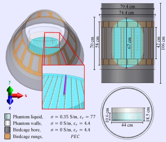
The CAD models used in simulations to mimic the performed experiment with the E‐field exposure generated by 1.5T RF body coil that is used in experiments. The wire trajectory and phantom position were altered slightly to match their respective experimental locations using the acquired MRI data, with the exception that the wires were always assumed to be perfectly aligned with the z‐axis

As long as the incident electric field distribution tangential to the implant, $E_{inc}$, is known and the resultant current distribution, $I_{ind}$ through the wire can be measured using MRI, the TM can be determined through the minimization given by Equation (5). In this minimization, the TM M is described by the attenuated wave model and characterized with parameters $c,{\mathrm{\Gamma }}_0,{\mathrm{\Gamma }}_L$, and ${\sigma }_{eff}$ The output of the minimization are the model parameters that best describe the complete TM M. The electric field exposure, $E_{inc}$, is a fixed characteristic of the measurement setup and does not depend on the implant being examined.

In an actual MRI acquisition the distribution of $\left|B_1^{+}\right|$ and the transceive phase16 are measurable. The distributions of these quantities in the vicinity of a wire can be used to determine the current.17, 18, 19, 20 The incident electric field distribution is obtained from simulations.

The simulations approximating the actual MRI experiment were validated by comparison of the $\left|B_1^{+}\right|$ and transceive phase distribution in the phantom without an implant. Therefore, the $B_1^{+}$ magnitude distribution was experimentally determined with a 3D dual TR actual flip angle (AFI) acquisition21 with 7 × 7 × 5 mm voxel size and a 30 ms TR extension on an initial repetition time of 9.1 ms on a 1.5 Tesla Philips Ingenia MR scanner (Philips Healthcare, Best, The Netherlands). With a FOV of 140 × 300 × 450 mm (APxFHxRL) and four signal averages, this acquisition took 192 s. The transceive phase was determined by the average phase of two 3D spoiled gradient echo acquisitions with opposing gradient polarities to correct for eddy current contributions22 and potential timing inaccuracies.23

The signal contributions from the receive array were removed using homogeneity correction with a coil sensitivity maps acquired in a reference scan. This ensures only transmit and receive sensitivities from the birdcage coil are present in the acquired data. The phase acquisitions have the same geometry as the AFI acquisition. Five echoes were acquired and used to correct for unwanted phase contributions from B₀ inhomogeneities16 that grow linearly in time. The resulting complex $B_1^{+}$ distribution without an implant present is used to validate equivalent simulations without an implant present. From these simulations, the incident electric field is determined.

In addition to the incident electric field, the induced current in the wire needs to be determined. The current is calculated from the $\left|B_1^{+}\right|$ distribution in the phantom with one of the implants present. These distributions were determined with the variable flip angle method24, 25 as this technique is better able to capture the large range of $\left|B_1^{+}\right|$ values present in the case of the wire immersed in the phantom at the expense of extra acquisition time. For this purpose a large range of 3D spoiled gradient echo images with various nominal flip angles17 were acquired. The spoiled gradient echo images had the same FOV as the AFI acquisition but a smaller voxel size of 1.9 × 1.9 × 5 mm to capture the rapid decay of the $\left|B_1^{+}\right|$ enhancement around the wire. The nominal flip angles were 0.25, 0.5,1, 2, 3, 4, 6, 10, 13, 16, 19, 22, 25, 30, 50, 75, 90, 120 degrees. The acquisitions had a repetition time of 30 ms leading to scan duration of 123 s per scan. From these acquisitions the $\left|B_1^{+}\right|$ was determined by fitting the signal from spoiled gradient echo acquisitions as function of flip angle to the data on a voxel by voxel basis17 using the following equation:

$$\text{Signal}\left(\overrightarrow{x}\right)\propto \frac{C_1\left(\overrightarrow{x}\right)\left(1-e^{-\raisebox{1ex}{$TR$}\!\left/ \!\raisebox{-1ex}{$T_1$}\right.}\right)\sin \left(C_2\left(\overrightarrow{x}\right)FA\right)}{1-e^{-\raisebox{1ex}{$TR$}\!\left/ \!\raisebox{-1ex}{$T_1$}\right.}\cos \left(C_2\left(\overrightarrow{x}\right)FA\right)}{e}^{-\raisebox{1ex}{$TE$}\!\left/ \!\raisebox{-1ex}{$T_2^{*}$}\right.}.$$ (6)

Here, $C_1\left(\overrightarrow{x}\right)$ is proportional to the receive sensitivity and $C_2\left(\overrightarrow{x}\right)$ is proportional to the $\left|B_1^{+}\left(\overrightarrow{x}\right)\right|$ distribution.The relaxation times were fixed parameters in the signal fit that were determined with a simultaneous multi spin echo interleaved with inversion recovery sequence.26 Subsequently an annulus of $\left|B_1^{+}\left(\overrightarrow{x}\right)\right|$ data around the wire was used to fit the $\left|B_1^{+}\left(\overrightarrow{x}\right)\right|$ artifact resulting from the interference of the complex magnetic fields due to the current and the background $B_1^{+}$ field. From the measured $\left|B_1^{+}\right|$ field modification, the current distribution along the wire is deduced. The phase difference between the $B_1^{+}$ magnetic field produced by current and the background $B_1^{+}$ field also follows from this fit. This difference in combination with the experimentally determined transceive phase distribution is used to compute the phase of the current. More details on this procedure can be found in the Supporting Information (and Supporting Information Figures S1 and S2).

Using the experimentally determined induced current distribution and the matched incident electric field distribution from simulations, the TM can be computed with Equation (5) similarly as was achieved in simulations. The bare and the capped wire were used as test implants in the MRI experiments.

4. RESULTS

4.1. Validation of the attenuated wave model

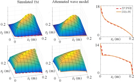
PWE‐simulated TMs and their fits using the attenuated wave model of the TM for the four investigated structures are shown in Figure 5. The agreement is very good with Pearson correlation coefficients exceeding 0.99 for all implants. This shows that the attenuated wave model is able to accurately capture the induced current in the investigated structures exposed to an incident electric field. Understandably, for symmetrical implants (1 and 4) the TM is also symmetrical.

Figure 5.

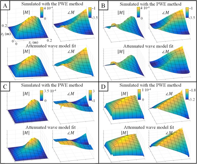
A–D, Validation of the attenuated wave model: the first row of each subfigure shows the TM that results from the piecewise excitation (PWE) simulations and the second row shows the fitted TM using the attenuated wave model. Note that the x‐ and y‐axis are the same for all plots. This figure demonstrates that the TM of all implants can be accurately characterized using the attenuated wave model (the Pearson correlation coefficient between fitted and simulated TMs was above 0.99 for all structures in both magnitude and phase). Structures A through D correspond to the ones shown in Figure 3

4.2. TF is contained in the TM

An excitation at the tip of an implant results in an induced current distribution that is proportional to the TF of the implant by virtue of the principle of reciprocity.10 Therefore, the first column of the TM is directly proportional to the TF of the implant. Figure 6 shows the first column of the fitted TM, M(z,0), in comparison to the TF from PWE simulations. The TF is by definition normalized to have unit integral value. In Figure 6, M(z,0) is normalized accordingly. The agreement between fitted M(z,0) and the TF confirms that the TN parameterized by a few parameters contains an accurate estimate of the TF in its first column.

Figure 6.

The TM contains the transfer function TF. The first column of the TM is directly proportional to the TF of the implant. M(z,0) is the current distribution in the implant when this distribution is induced by an electric field excitation at the tip. This is proportional to the TF by virtue of the principle of reciprocity.9 The normalized TF, i.e., to have a unit integral, determined with the PWE method is shown as a dashed red line in the figure of the right. The normalized TF according to the fit of the TM is shown as a solid orange line in this plot. The agreement between both TFs shows that the attenuated wave description keeps the TF intact

4.3. MRI‐based implant TM determination

In simulations the relevant electromagnetic quantities E_inc and I_ind are readily available. If these quantities are known, Equation (5) can be used to determine the TM. In MRI experiments these electromagnetic quantities are not directly available. However, they can be derived from measurements and simulations. The conductivity of the phantom is determined from a phase only EPT reconstruction using the measured transceive phase distribution27 in a centered ROI and used in simulations. These simulated $\left|B_1^{+}\right|$ and transceive phase, i.e., $\angle B_1^{+}{B}_1^{-*}$, distributions along with their experimentally determined counterparts are shown in Figure 7. Data show that the overall distributions are very similar (R = 0.96) although some slight differences do exist. For example, the right top corner of the $\left|B_1^{+}\right|$ distribution in the transverse plane seems to be more enhanced in experiments than in simulations. However, these deviations are minor and are not expected to introduce considerable errors in the resulting TMs.

Figure 7.

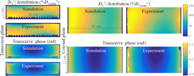
The top row shows the simulated and measured $\left|{\mathrm{B}}_1^{+}\right|$ distributions in percentage of nominal flip angle in the phantom without a wire. The $\left|{\mathrm{B}}_1^{+}\right|$ distribution was experimentally determined with a 3D dual TR actual flip angle (AFI) acquisition21 with 7 × 7 × 5 mm voxel size and a 30 ms TR extension on an initial repetition time of 9.1 ms. The bottom row shows the simulated and measured transceive phase distributions in radians. The transceive phase was experimentally determined by averaging the phase of two 3D spoiled gradient echo acquisitions with opposing gradient polarities to correct for eddy current contributions22 and potential timing inaccuracies.23 Simulations and measurements show good agreement (the Pearson correlation coefficients are R = 0.90 and R = 0.98 for the magnitude and the phase, respectively). Note that the coronal view does not show the entire phantom due to experimental limitations like ${\mathrm{B}}_1^{+}$ coverage, B₀ homogeneity, and gradient linearity

In Figure 8 the $\left|B_1^{+}\right|$ distribution in the phantom with an embedded implant is shown. The agreement between the distributions in Figure 8 provides additional confidence in the accuracy of the simulations and the proposed method. A close‐up of the $\left|B_1^{+}\right|$ modulation due to the alteration of the RF field by the implant is also shown. This artifact is used to determine the current running in the wire (see the Supporting Information for more details).

Figure 8.

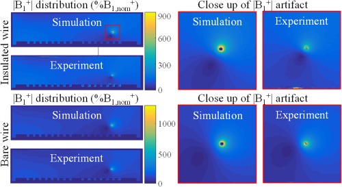
Simulated and measured $\left|{\mathrm{B}}_1^{+}\right|$ distributions in percentage of nominal flip angle inside the phantom when an implant is present. A close up of $\left|{\mathrm{B}}_1^{+}\right|$ artifact around the wires is shown on the right. This artifact is used to determine I_ind as described in the Supporting Information

The currents are determined from the measured $\left|{\mathrm{B}}_1^{+}\right|$ distributions close to the wire. These measured current distributions along the wires are subsequently used to determine the TM of the bare and the insulated wire with Equation (5) using a derivative‐free, nonlinear least squares optimizer (fminsearch). The solution was the one with lowest residual from a set of 256 minimizations performed with equidistantly distributed start points. The same (overall) minimum was found for 29 (11.3%) and 97 (37.9%) of the 256 start values for the insulated and bare wire, respectively. The frequent occurrence of the found minimum with lowest residual suggests convergence to a global minimum in the investigated search space.

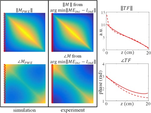
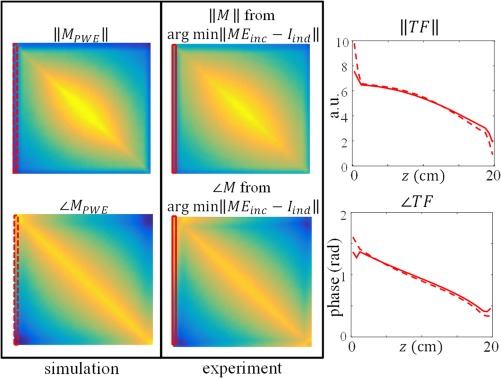
The first and second columns in Figure 9 (bare wire) and 10 (insulated wire) show the gold standard TM from PWE simulations and the experimentally determined TM respecively. The normalized TFs that follow from these matrices are plotted in the third column of Figures 9 and 10.

Figure 9.

The first column in this figure shows the gold standard TM from PWE simulations for the bare wire (structure A in Figure 3). The second column shows the TM resulting from the minimization in Equation (5) given the current measured with MRI and the incident electric field from simulations. The plot in the third column displays the normalized transfer function from measurements (solid line) and simulations (dashed line)

Figure 10.

The first column in this figure shows the gold standard TM from PWE simulations for the insulated wire (structure D in Figure 3). The second column shows the TM resulting from the minimization in Equation (5) given the current measured with MRI and the incident electric field from simulations. The plot in the third column displays the normalized transfer function from measurements (solid line) and simulations (dashed line)

5. DISCUSSION

This work has presented an alternative method to measure the TF of medical implants using MRI. It does not require alterations to the implant and is, therefore, a substantial improvement in comparison to the MRI‐based method that was presented earlier.11 Because the electric field is not localized at the tip but will be distributed along the entire implant during an MRI exam, an alternative formalism has been introduced: the TM. Where the TF can be used to evaluate the electric field at the tip, the TM can be used to determine the total current/electric field anywhere along the implant for a given incident, tangential electric field.

The measurement of the TM by MRI without modification to the implant is only feasible by application of the attenuated wave model which drastically reduces the number of unknowns of this matrix. The attenuated wave description was successfully validated with simulations. With this reduction of unknowns one MRI measurement of the induced current is sufficient to determine the TM. The TF is contained in the TM as its first row and is hence simultaneously determined. As an additional advantage, the TM also allows identification of other locations that potentially exhibit significant heating along the implant. It is known from practice that localized heating can occur for instance also at impedance transitions in the implant where charge accumulation and thus electric field concentration can take place.28 Other models29, 30, 31 are available that give an analytical description for the current in a wire due to an incident electric field. With some modifications these models could be used in a similar way as the attenuated wave model.

For the examined structures the presented method was able to accurately measure their TFs (the Pearson correlation coefficients were 0.929 and 0.926 for the bare and the insulated wire, respectively). Given a constant electric field with a worst case phase distribution, i.e., a phase distribution with opposite sign as the phase of the gold standard simulated TFs, the measured TFs would lead to an underestimation of the scattered electric field around the tip of 2.1% and 5.3%, respectively, in comparison to the simulated cases.

The descriptive power of the attenuated wave model for realistic implants is a topic for future research. The number of parameters to describe the response might increase because the wave number can be spatially varying. This will lead to more complicated minimization problems with possible additional numerical challenges. In addition to their potentially more complicated descriptions realistic implants might produce susceptibility artifacts that need to be mitigated. This will especially an issue for implants nonparallel with the B₀ field. Many mitigation strategies for metal artifact reduction exist,32 but testing these is beyond the scope of the presented method.

Nonetheless, for the tested generic copper structures the high correlation coefficients between the measured and simulated TFs confirm that the normalized TF can be accurately determined with the proposed method. In these TMs, still some discrepancies are visible for the current estimates close to the tips of the implant. We believe that this is a consequence of the difficulties to accurately determine the low currents and thus low wire $\left|{\mathrm{B}}_1^{+}\right|$ fields near the ends of the wires. Also discrepancies in the phases of the simulated and measured currents are visible. Two potential causes are conceivable. First, the approximation that the transmit and receive phases are equal, the so called transceive phase assumption as used also in EPT, introduces a small error. This approximation is needed to estimate the background phase of the ${\mathrm{B}}_1^{+}$ field created by the birdcage. Second, the phase difference between the current in the wire and the background field that follows from the fit of the $\left|B_1^{+}\right|$ artifact, again suffers from the low current magnitudes near the ends of the implant.

Another potential source of inaccuracy are physical deviations between the experiments and the simulations. Some differences between simulations and experiments are inevitably present. For example the wires are assumed to be perfectly aligned with the main magnetic field and perfectly straight. Despite attempts to reach this alignment in practice small angles (less than 5 °) with the main magnetic field were present. This leads to errors in the incident electric field, because this is spatially varying, as well as the measured current as it is a projection of the true current on the main magnetic field direction. Other potential sources of inaccuracy are differences in material properties between simulations and experiments, predominantly the phantom liquid and the insulation of the insulated wire.

The presented method for TF determination only requires the wire to be aligned with the z‐axis because the measurement of the induced current relies on this assumption. Nevertheless, the measurement of induced currents that are not aligned with the z‐axis is in principle possible, because the current will always have a nonzero projection on ${\mathrm{B}}_1^{+}$. Extension of the current determination method for currents that are not aligned with the z‐axis is a topic for future research. This would allow determination of the TF in the case of more realistic lead trajectories.

Most of the aforementioned physical sources of inaccuracy can be mitigated. For example the alignment errors might be reduced with dedicated placeholders for the implants or adaptations to the phantom. More accurate knowledge of the material properties can be attained with dedicated hardware, when available, and could improve agreement between measurements and simulations. Furthermore, a choice was made to determine the current in the wire based on magnitude data. Other approaches, e.g., phase‐based current determination20 or a hybrid method, are possible and might perform better. This also holds for the multi flip angle $\left|B_1^{+}\right|$ mapping technique. There are numerous methods21, 33, 34 to measure $\left|B_1^{+}\right|$ distributions that could outperform the applied technique.

In addition to these incremental technical and experimental improvements, MR‐based TM determination could benefit from other advances. For example, although the induced current along the implant I_ind is determined from an MRI measurement, the incident electric field E_inc is obtained from simulations. Potentially, simulations can be avoided by means of MRI‐based E_z‐field determination.35 In this way also the incident, z‐component of the electric field can be determined experimentally using the MRI experiment without an implant in the phantom. Although difficulties are expected taking spatial derivatives of the measured, noisy $B_1^{+}$ field.

Another limitation is the necessity to perform a separate MRI acquisition without the presence of an implant field to characterize the test setup and therewith validate the exposure field. Note that although a given ${\mathrm{B}}_1^{+}$ magnitude distribution does not uniquely define a corresponding longitudinal electric field distribution, the combination with phase measurements (i.e., the full complex ${\mathrm{B}}_1^{+}$ distribution) does. In principle, the scattered and incident electric field could be separated based on their different spatial dependencies. The scattered field drops off radially from the wire and has its source inside the phantom.

Contrarily, the incident field is created by sources outside the phantom and can be decomposed in spherical and cylindrical basis functions that are solutions to the source free (or homogeneous) Helmholtz equation.36 This distinctly different spatial dependency potentially allows reconstruction of both the scattered and incident fields from a single scan with the wire present. However, again knowledge of the complex $B_1^{+}$ distribution is required with the implant present, which is hard to attain because its presence makes the transmit and receive phase distinctly different. Multi‐transmit methods can be used to remove this obstacle.37

Currently, inaccuracies of which the significance cannot be exactly gauged, are introduced when a TF measured in a phantom experiment or in simulations are applied to evaluate the heating of an implant in a human body (where the implant's characteristics will be different due to varying loading conditions). The presented method allows TM and hence TF determination in more realistic situations provided that the incident electric fields are assessable and makes it possible to experimentally examine the significance of the uncertainties introduced with this simplification. Furthermore, the TM concept can be used in transmit field modification strategies19, 38, 39, 40 to minimize the induced currents in the implant. Most importantly it allows determination of the TF without the need for electric field probes or alterations to the implant with a high spatial resolution that has the potential to be used in solids. With considerable modifications and additional work to the method presented here it is conceivable that extensions to TF determination in heterogeneous media and even animal tests can be made.

6. CONCLUSIONS

We have presented a method to measure the TF of an implant in a designated phantom using an MRI scanner without alterations to the implant. The Pearson correlation coefficients between measured and the simulated TFs were 0.929 and 0.926 for a 20 cm bare and a 20 cm insulated wire, respectively.

For this method, the concept of the TM was introduced. This matrix relates the induced current along an implant to an incident E‐field distribution. This matrix contains the TF in its first column. The measurement of this matrix by MRI is feasible by application of an attenuated wave model which drastically reduces the number of unknowns of this matrix. The applicability of this model for (partially) insulated wires in a homogeneous medium was verified with numerical simulations. Using a validated experimental test setup in which the electric field exposure is known, one MRI measurement of the induced current is sufficient to determine the TM and hence also the TF of an simple implant model. For application of the presented method to TF determination of realistic (and often more complex) implants the TM model needs to be extended which might prove to be a nontrivial task.

The introduced TM enables MRI‐based TF determination without hardware alterations to implant or scanner. This MRI‐based method opens up possibilities to determine TFs in more realistic scenarios like solid tissues, heterogeneous media and test animals.

Supporting information

FIGURE S1. The real part of the first three waves in geometric series of the attenuated wave model that is used to derive parameterizations for the transfer functions and matrices of the bare and (partially) insulated wires. In this situation a wire that has a constant wave number along its length is considered.

FIGURE S2. The principle behind the |B1+| mapping techniques that is able to capture a high dynamic range of actual flip angles. The same scan is performed with various flip angles and the acquired signal as function of requested flip angles is fitted voxel wise the signal for spoiled gradient echo acquisitions.2 The example fit for a voxel close to the wire (red) and further away from the wire (blue) are shown. If this fit is performed voxel wise distributions for C₁ and C₂ appear which are shown below the example fit.

FIGURE S3. Current determination from the $\left|{\mathrm{B}}_1^{+}\right|$ artefact around a wire. An annulus of |B1+| data (from the multi‐flip angle analysis) centered around the wire is fitted on a slice by slice bases with Equation 2.The full $\left|{\mathrm{B}}_1^{+}\right|$ distribution in the phantom is shown in the top left corner. A close‐up of the selected annulus of $\left|{\mathrm{B}}_1^{+}\right|$ data and its fit is shown in the bottom left corner. On the right this data and its fit is graphically shown as function of radial distance from the wire.

Tokaya JP, Raaijmakers AJE, Luijten PR, Berg CAT. MRI‐based, wireless determination of the transfer function of a linear implant: Introduction of the transfer matrix. Magn Reson Med. 2018;80:2771–2784. 10.1002/mrm.27218

REFERENCES

- 1. Henderson JM, Tkach J, Phillips M, Baker K, Shellock FG, Rezai AR. Permanent neurological deficit related to magnetic resonance imaging in a patient with implanted deep brain stimulation electrodes for Parkinson's disease: case report. Neurosurgery. 2005;57:E1063; discussion E1063. [DOI] [PubMed] [Google Scholar]
- 2. Yeung CJ, Susil RC, Atalar E. RF heating due to conductive wires during MRI depends on the phase distribution of the transmit field. Magn Reson Med. 2002;48:1096‐1098. [DOI] [PubMed] [Google Scholar]
- 3. Bottomley PA, Kumar A, Edelstein WA, Allen JM, Karmarkar PV. Designing passive MRI‐safe implantable conducting leads with electrodes. Med Phys. 2010;37:3828‐3843. [DOI] [PubMed] [Google Scholar]
- 4. Nordbeck P, Fidler F, Weiss I, et al. Spatial distribution of RF‐induced E‐fields and implant heating in MRI. Magn Reson Med. 2008;60:312‐319. [DOI] [PubMed] [Google Scholar]
- 5. Langman DA, Goldberg IB, Judy J, Paul Finn J, Ennis DB. The dependence of radiofrequency induced pacemaker lead tip heating on the electrical conductivity of the medium at the lead tip. Magn Reson Med. 2012;68:606‐613. [DOI] [PubMed] [Google Scholar]
- 6. Yeung CJ, Susil RC, Atalar E. RF safety of wires in interventional MRI: using a safety index. Magn Reson Med. 2002;47:187‐193. [DOI] [PubMed] [Google Scholar]
- 7. ISO/TS 10974:2012(en) . Assessment of the safety of magnetic resonance imaging for patients with an active implantable medical device. https://www.iso.org/standard/46462.html. Accessed April 8, 2018.
- 8. Park SM, Kamondetdacha R, Nyenhuis JA. Calculation of MRI‐induced heating of an implanted medical lead wire with an electric field transfer function. J Magn Reson Imaging. 2007;26:1278‐1285. [DOI] [PubMed] [Google Scholar]
- 9. Zastrow E, Capstick M, Cabot E. Piece‐wise excitation system for the characterization of local RF‐induced heating of AIMD during MR exposure. Presented at 2014 International Symposium on Electromagnetic Compatibility, Tokyo, Japan (EMC'14/Tokyo), 2014. pp. 241‐244.
- 10. Feng S, Qiang R, Kainz W, Chen J. A technique to evaluate MRI‐induced electric fields at the ends of practical implanted lead. IEEE Trans Microwve Theory Tech. 2015;63:305‐313. [Google Scholar]
- 11. Tokaya JP, Raaijmakers AJE, Luijten PR, Bakker JF, van den Berg CAT. MRI‐based transfer function determination for the assessment of implant safety. Magn Reson Med. 2017;78:2449‐2459. [DOI] [PubMed] [Google Scholar]
- 12. Yeh P. Optical Waves in Layered Media. Hoboken: Wiley; 1988. [Google Scholar]
- 13. Arfken GB, Weber HJ, Harris FE. Mathematical Methods for Physicists. Amsterdam: Elsevier; 2013. [Google Scholar]
- 14. Katscher U, van den Berg CAT. Electric properties tomography: biochemical, physical and technical background, evaluation and clinical applications. NMR Biomed. 2017;30:1‐15. [DOI] [PubMed] [Google Scholar]
- 15.F2182‐11a A. Standard test method for measurement of radio frequency induced heating on or near passive implants during magnetic resonance imaging. https://www.astm.org/Standards/F2182.htm. Accessed April 8, 2018.
- 16. van Lier AL, Brunner DO, Pruessmann KP, et al. B 1 + Phase mapping at 7 T and its application for in vivo electrical conductivity mapping. Magn Reson Med. 2012;67:552‐561. [DOI] [PubMed] [Google Scholar]
- 17. van den Bosch MR, Moerland MA, Lagendijk JJ, Bartels LW, van den Berg CA. New method to monitor RF safety in MRI‐guided interventions based on RF induced image artefacts. Med Phys. 2010;37:814‐821. [DOI] [PubMed] [Google Scholar]
- 18. Venook R, Overall W, Shultz K, Conolly S, Pauly J, Scott G. Monitoring induced currents on long conductive structures during MRI. In Proceedings of the 16th Annual Meeting of ISMRM, Toronto, Canada, 2008. Abstract 898.
- 19. Overall WR, Pauly JM, Stang PP, Scott GC. Ensuring safety of implanted devices under MRI using reversed RF polarization. Magn Reson Med. 2010;64:823‐833. [DOI] [PMC free article] [PubMed] [Google Scholar]
- 20. Griffin GH, Anderson KJT, Celik H, Wright GA. Safely assessing radiofrequency heating potential of conductive devices using image‐based current measurements. Magn Reson Med. 2015;73:427‐441. [DOI] [PubMed] [Google Scholar]
- 21. Yarnykh VL. Actual flip‐angle imaging in the pulsed steady state: a method for rapid three‐dimensional mapping of the transmitted radiofrequency field. Magn Reson Med. 2007;57:192‐200. [DOI] [PubMed] [Google Scholar]
- 22. Bernstein MA, King K, Zhou X. Handbook of MRI Pulse Sequences. Magnetic Properties of Tissues: Theory and Measurement. New York: Elsevier; 2004. [Google Scholar]
- 23. Klassen LM, Menon RS. Robust automated shimming technique using arbitrary mapping acquisition parameters (RASTAMAP). Magn Reson Med. 2004;51:881‐887. [DOI] [PubMed] [Google Scholar]
- 24. Barker GJ, Simmons A, Arridge SR, Tofts PS. A simple method for investigating the effects of non‐uniformity of radiofrequency transmission and radiofrequency reception in MRI. Br J Radiol. 1998;71:59‐67. [DOI] [PubMed] [Google Scholar]
- 25. Alecci M, Collins CM, Smith MB, Jezzard P. Radio frequency magnetic field mapping of a 3 Tesla birdcage coil: experimental and theoretical dependence on sample properties. Magn Reson Med. 2001;46:379‐385. [DOI] [PubMed] [Google Scholar]
- 26. in den Kleef JJ, Cuppen JJ. RLSQ: T1, T2, and?rho calculations, combining ratios and least squares. Magn Reson Med. 1987;5:513‐524. [DOI] [PubMed] [Google Scholar]
- 27. Wen H. Noninvasive quantitative mapping of conductivity and dielectric distributions using RF wave propagation effects in high‐field MRI. Proc. SPIE 5030, Medical Imaging 2003: Physics in Medical Imaging. 2003. 10.1117/12.480000. Accessed April 8, 2018. [DOI]
- 28. Gupte AA, Shrivastava D, Spaniol MA, Abosch A. MRI‐related heating near deep brain stimulation electrodes: more data are needed. Stereotact Funct Neurosurg. 2011;89:131‐140. [DOI] [PMC free article] [PubMed] [Google Scholar]
- 29. Shen LC, Wu TT, King RWP. A simple formula of current in dipole antennas. IEEE Trans Antennas Propag. 1968;AP‐16:542‐547. [Google Scholar]
- 30. King RWP, Trembly BS, Strohbehn JW. The electromagnetic field of an insulated antenna in a conducting or dielectric medium. IEEE Trans Microw Theory Tech. 1983;31:574‐583. [Google Scholar]
- 31. Acikel V, Atalar E. Modeling of radio‐frequency induced currents on lead wires during MR imaging using a modified transmission line method. Med Phys. 2011;38:6623‐6632. [DOI] [PubMed] [Google Scholar]
- 32. Hargreaves BA, Worters PW, Pauly KB, Pauly JM, Koch KM, Gold GE. Metal‐induced artifacts in MRI. AJR Am J Roentgenol. 2011;197:547‐555. [DOI] [PMC free article] [PubMed] [Google Scholar]
- 33. Sacolick LI, Wiesinger F, Hancu I, Vogel MW. B1 mapping by Bloch‐Siegert shift. Magn Reson Med. 2010;63:1315‐1322. [DOI] [PMC free article] [PubMed] [Google Scholar]
- 34. Nehrke K, Versluis MJ, Webb A, Börnert P. Volumetric B1 + mapping of the brain at 7T using DREAM. Magn Reson Med. 2014;71:246‐256. [DOI] [PubMed] [Google Scholar]
- 35. Buchenau S, Haas M, Splitthoff DN, Hennig J, Zaitsev M. Iterative separation of transmit and receive phase contributions and B 1 + ‐based estimation of the specific absorption rate for transmit arrays. MAGMA. 2013;26:463‐476. [DOI] [PubMed] [Google Scholar]
- 36. Sbrizzi A, Hoogduin H, Lagendijk JJ, Luijten P, Van Den Berg CAT. Robust reconstruction of B1 + maps by projection into a spherical functions space. Magn Reson Med. 2014;71:394‐401. [DOI] [PubMed] [Google Scholar]
- 37. Katscher U, Findeklee C, Voigt T. B1‐based specific energy absorption rate determination for nonquadrature radiofrequency excitation. Magn Reson Med. 2012;68:1911‐1918. [DOI] [PubMed] [Google Scholar]
- 38. Eryaman Y, Turk EA, Oto C, Algin O, Atalar E. Reduction of the radiofrequency heating of metallic devices using a dual‐drive birdcage coil. Magn Reson Med. 2013;69:845‐852. [DOI] [PubMed] [Google Scholar]
- 39. McElcheran CE, Yang B, Anderson KJT, Golenstani‐Rad L, Graham SJ. Investigation of parallel radiofrequency transmission for the reduction of heating in long conductive leads in 3 Tesla magnetic resonance imaging. PLoS One. 2015;10:1‐21. [DOI] [PMC free article] [PubMed] [Google Scholar]
- 40. Golestanirad L, Keil B, Angelone LM, Bonmassar G, Mareyam A, Wald LL. Feasibility of using linearly polarized rotating birdcage transmitters and close‐fitting receive arrays in MRI to reduce SAR in the vicinity of deep brain simulation implants. Magn Reson Med. 2017;77:1701‐1712. [DOI] [PMC free article] [PubMed] [Google Scholar]
Associated Data
This section collects any data citations, data availability statements, or supplementary materials included in this article.
Supplementary Materials