The optimal mating distance resulting from heterosis and genetic incompatibility

Offspring are fittest when parents are genetically neither too close nor too distant from each other.

Abstract

Theory predicts that the fitness of an individual is maximized when the genetic distance between its parents (i.e., mating distance) is neither too small nor too large. However, decades of research have generally failed to validate this prediction or identify the optimal mating distance (OMD). Respectively analyzing large numbers of crosses of fungal, plant, and animal model organisms, we indeed find the hybrid phenotypic value a humped quadratic polynomial function of the mating distance for the vast majority of fitness-related traits examined, with different traits of the same species exhibiting similar OMDs. OMDs are generally slightly greater than the nucleotide diversities of the species concerned but smaller than the observed maximal intraspecific genetic distances. Hence, the benefit of heterosis is at least partially offset by the harm of genetic incompatibility even within species. These results have multiple theoretical and practical implications for speciation, conservation, and agriculture.

INTRODUCTION

The genetic distance between the two parents of an individual, or mating distance D, influences the individual’s fitness via two competing mechanisms. On the one hand, increasing D is beneficial because of the phenomenon of heterosis, which is also known as hybrid vigor (1–4). On the other hand, too large of a D is harmful owing to genetic incompatibility (5–7). It is thus believed that the fitness (or its proxy) of a genotype is a hump-shaped function of D, culminating at an intermediate value referred to as the optimal mating distance (OMD) (8). Numerous studies have attempted to verify this belief (9–16), but all failed except two. In the first exception (15), however, D was approximated by geographic distance (11), and genetic incompatibility was detected under low but not high D (15), rendering the conclusion uncertain. In the second exception, D was estimated using the electrophoretic data of only eight allozyme loci; the low resolution prevented an unequivocal assessment of the OMD relative to the level of intraspecific genetic diversity (12). The difficulties in confirming the predicted humped relationship were probably contributed by the lack of reliable D estimates. Furthermore, given D, the fitness of a hybrid varies greatly depending on its genotype. Hence, a large number of crosses are required to accurately estimate the expected hybrid fitness at each D. Given these considerations, we collected from the literature large sets of relevant genotype and phenotype data in an attempt to test the hypothesized relationship between D and hybrid fitness and to estimate the OMD.

RESULTS

Theoretical prediction of hybrid performance as a function of mating distance

Fitness is a compound trait consisting of multiple components. Most studies measure one to several key components of fitness such as the maximum growth rate of microbes, shoot weight of plants, and body weight of animals. The phenotypic value of a fitness-related trait is commonly referred to as “performance.” To allow among-cross comparisons, for a given trait, we examined the fractional increase in hybrid performance relative to the average performance of its homozygous parents by $\mathit{F}=(\mathit{H}-\frac{{\mathit{P}}_1+{\mathit{P}}_2}{2})/\left(\frac{{\mathit{P}}_1+{\mathit{P}}_2}{2}\right)$, where H is the performance of the hybrid and P₁ and P₂ are the performances of the two parents. When D = 0, the hybrid and the two homozygous parents are genetically identical to one another; thus, F is expected to be 0. Under pure genetic additivity, H is expected to equal the average of P₁ and P₂, resulting in F = 0 regardless of D. Heterosis arises from genetic interactions between the paternal and maternal alleles of the same loci (via dominance and overdominance) and/or different loci (via positive intergenic epistasis) (4). Genetic incompatibility similarly originates from allelic interactions at the same loci (via underdominance) and/or different loci (via negative intergenic epistasis). Here, overdominance refers to the scenario where the heterozygote at a locus is fitter than both homozygotes, whereas underdominance refers to the scenario where the heterozygote at a locus is less fit than both homozygotes. At any locus, if the paternal and maternal alleles differ, either both of them are derived from their common ancestral allele at their coalescence or only one of them is derived whereas the other is ancestral. In the hybrid, the number of genetic interactions between an ancestral allele from one parent and a derived allele from the other parent is expected to rise linearly with D, whereas the number of interactions between two derived alleles is expected to rise in proportion to D². It can be shown that dominance most likely occurs between one ancestral allele and one derived allele, whereas the other interactions mentioned most likely occur between two derived alleles (see Materials and Methods). Therefore, the expected number of dominance interactions is proportional to D, while the expected numbers of overdominance, underdominance, positive intergenic epistasis, and negative intergenic epistasis are all proportional to D². High-order interactions are ignored here because considering them substantially increases the complexity of the model and difficulty in model selection. Because the effect size of an interaction is expected to be independent of D, the joint effect of heterosis and genetic incompatibility should result in F = aD + bD², where the first term reflects heterosis due to dominance while the second term reflects the combined effect of (i) heterosis arising from overdominance and positive intergenic epistasis and (ii) genetic incompatibility arising from underdominance and negative intergenic epistasis. If |aD| >> |bD²|, then F ≈ aD, which monotonically changes with D. If |aD| << |bD²|, then F ≈ bD², which also monotonically changes with positive D. Under the condition that a is positive, b is negative, and |aD| is comparable with |bD²|, F is a hump-shaped function of D and OMD = −0.5a/b.

On the basis of the above formulation, we considered three competing models: (I) F = aD, (II) F = bD², and (III) F = aD + bD², where a and b are model parameters to be estimated. Model I has only the linear term, meaning that F is entirely caused by dominance-based heterosis; model II has only the quadratic term, implying the absence of dominance-based heterosis; and model III contains both terms. We assess which model best explains a dataset by the coefficient of determination (R²). Because models I and II are both special cases of model III, we used likelihood ratio tests (LRTs) to examine whether the first two models can be statistically rejected in favor of model III.

Model III is favored in yeast

We started by analyzing 231 crosses of the yeast Saccharomyces cerevisiae that included estimates of the maximum growth rates of all parents and hybrids in 11 different liquid media (14). We first studied the mean F from the 11 environments. D is measured by the number of single-nucleotide polymorphisms (SNPs) between parental genomes divided by the total number of nucleotide sites considered (see Materials and Methods).

Because F varies greatly among crosses of similar D as a result of different genetic interactions in different hybrids due to different parental genotypes, our theoretical models relate D with expected F. Note that binning crosses of similar D does not introduce statistical bias to parameter estimation and allows a robust model evaluation by avoiding disproportionally large influences from numerous hybrids of similar mating distances (see Materials and Methods). Therefore, we binned the hybrids using a window size of D = 10⁻³ and computed the average F and average D of all hybrids in each window. We used least-squares regression to fit the three models to the binned data, respectively (Fig. 1A). Model III has an impressive R² of 0.85, whereas the corresponding values are negative for the other two models (Table 1), indicating that these models, assuming monotonic changes of F with D, perform even worse than the obviously incorrect null model that F is independent of D. Using weighted least-squares (WLS) regression (see Materials and Methods) also supports model III (Table 1). Furthermore, LRT showed that model III fits the data significantly better than the other two models (Table 1). These results are robust to different window sizes including not binning the data (table S1). Under model III, a clear hump-shaped relationship is observed between the mean F and D. The estimated OMD = 4.5 × 10⁻³ (Fig. 1A), with a 95% confidence interval of 4.2 × 10⁻³ to 4.9 × 10⁻³ (table S1). This OMD of 4.5 × 10⁻³ equals a genetic distance of 4.5 differences per 1000 nucleotides. To minimize the influence of potentially poorly measured growth rates of individual parental strains on the estimation of F of all crosses involving the parent, we performed a jackknife resampling of parental strains (by individually removing the 22 parental strains and all crosses involving the parental strain from the analysis), yielding OMD estimates between 4.27 × 10⁻³ and 4.85 × 10⁻³. S. cerevisiae has a genome-wide nucleotide diversity (π) of 4.3 × 10⁻³ and a maximal intraspecific genetic distance (D_max) of 9.6 × 10⁻³ after the exclusion of reproductively isolated Chinese strains (see Materials and Methods). Hence, the estimated OMD is slightly greater than π but much smaller than D_max.

Fig. 1. Hump-shaped relationship between mating distance (D) and hybrid performance (F) in the fungus S. cerevisiae across 11 environments (see Materials and Methods for details of the environments).

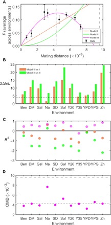
(A) The D-F relationship when F is measured by the average maximum growth rate in 11 environments. The mean and SE of F are shown by black squares and associated error bars, respectively. The fitted D-F curves under different models are shown in different colors. Nucleotide diversity (π) and maximal intraspecific genetic distance observed (D_max) are indicated by vertical dotted and dashed lines, respectively. Statistics of model fitting are provided in Table 1. (B) Twice the difference in ln(likelihood) between model III and model I (orange) or II (green) under each environment. The larger the difference, the fitter model III is relative to the model being compared. The horizontal black dashed line shows statistical significance at the 5% level. The x axis lists environments. (C) Model fitting for the D-F relationship in each of the 11 environments. Color coding is the same as in (A). The higher the R², the fitter the model is to the data. The horizontal black line indicates R² = 0. (D) The estimated OMD in each environment. π and D_max are indicated by horizontal dotted and dashed lines, respectively. Note that the term OMD does not apply in the medium “Ben” (see the main text and fig. S1).

Table 1. Fitting of the three models to the S. cerevisiae data averaged across 11 environments.

Models	R2 (R2WLS)*	2ΔlnL†	P‡	OMD [CI§] (OMDWLS) (×10−3)
I	−0.65 (0.30)	19.2	1.2 × 10−5
II	−2.40 (−0.39)	24.9	6.0 × 10−7
III	0.85 (0.95)			4.5 [4.2–4.9] (4.6)

*The coefficient of determination (R²) becomes negative when the fitted model performs worse than the mean of the variable. R²_WLS is the R² under WLS regression in the weighted space.

†Twice the difference in ln(likelihood) between model III and the model being compared.

‡P values of LRTs are determined using chi-square tests with 1 df.

§95% confidence interval of the OMD.

When the data from different environments were separately analyzed, LRTs showed that model III significantly outperforms the other two models in 10 of the 11 environments (except for the NaCl environment; Fig. 1B). R² of model III is higher than those of the other models in all 11 environments, and R² of model III is positive in 10 of the 11 environments (except for the Y35 medium; Fig. 1C). However, in the benomyl (Ben) medium, the curve under model III is not hump shaped but is U shaped (fig. S1). Ben is a synthetic fungicide that targets microtubules (14). It is possible that Ben penalizes fast-growth strains more than slow-growth strains, resulting in a U-shaped curve. In the 10 environments (except for NaCl) where LRTs find model III significantly fitter than the other two models, OMD is in the range of 3.2 ×10⁻³ to 5.3 × 10⁻³ (Fig. 1D). All of these OMDs are lower than D_max and many are close to π.

To further verify the above results, we analyzed another yeast dataset (17), which included the measures of three growth traits (growth rate, negative lag time, and growth efficiency) in 56 environments from 28 crosses. Because the number of crosses is relatively small, we averaged F from all environments to minimize the estimation error of F. For each of the three traits, model III fits the data significantly better than the other two models (table S2), and the humped curve is apparent under model III (fig. S2). The OMDs for the three traits are 6.3 × 10⁻³, 4.4 × 10⁻³, and 5.4 × 10⁻³, respectively (table S2), between π and D_max.

Recently, Bernardes et al. (18) studied heterosis in Saccharomyces paradoxus, the sister species of S. cerevisiae. Their data included the growth rates of hybrids relative to their two parents for 27 intraspecific crosses. These crosses form three separated groups in terms of mating distances: 0.006 to 0.0021 (13 crosses), 0.0112 to 0.0123 (7 crosses), and 0.0366 to 0.0380 (7 crosses). The group with intermediate mating distances shows the highest mean relative hybrid growth rate, suggesting the existence of an intraspecific OMD in S. paradoxus. However, the data are too sparse to allow reliably estimating OMD.

Model III is favored in Arabidopsis

To examine the generality of the hump-shaped relationship between D and expected F, we analyzed 200 crosses of the model plant Arabidopsis thaliana (13). We again estimated D by the number of SNPs per site in the A. thaliana genome (see Materials and Methods). Four fitness-related traits were measured for all parents and hybrids: shoot fresh weight, rosette diameter, leaf area, and leaf number at 14 days after sowing (13). We binned hybrids using a window size of D = 0.8 × 10⁻³. For each of the four traits, R² is negative for models I and II but positive for model III (Table 2). Using WLS regression also supports model III (Table 2). Furthermore, for each trait, LRTs showed that model III fits the data significantly better than the other two models (Table 2), and the fitted curve under model III is hump shaped (Fig. 2). These results are robust to different window sizes including not binning the data (table S3). The OMDs for the four traits estimated under model III are within a narrow range of 5.2 × 10⁻³ to 6.2 × 10⁻³ (Table 2 and Fig. 2), which are close to A. thaliana’s π (5.4 × 10⁻³) but smaller than its D_max (8.5 × 10⁻³) (see Materials and Methods).

Table 2. Fitting of the three models to the A. thaliana data.

Traits	Models	R2 (R2WLS)*	2ΔlnL†	P‡	OMD [CI§] (OMDWLS) (×10−3)
Shoot weight
	I	−4.15 (0.91)	14.5	1.4 × 10−4
	II	−16.20 (0.69)	21.7	3.1 × 10−6
	III	0.54 (0.99)			5.9 [4.8–9.7] (5.8)
Rosette diameter
	I	−2.32 (0.89)	10.7	1.1 × 10−3
	II	−7.38 (0.67)	16.2	5.6 × 10−5
	III	0.44 (0.98)			5.2 [4.7–7.5] (5.5)
Leaf area
	I	−6.26 (0.88)	17.8	2.4 × 10−5
	II	−19.50 (0.60)	24.1	9.4 × 10−7
	III	0.63 (1.00)			5.3 [4.7–7.1] (5.5)
Leaf number
	I	−1.34 (0.96)	8.1	4.5 × 10−3
	II	−6.50 (0.86)	15.1	1.0 × 10−4
	III	0.39 (0.99)			6.2 [−19.9–44.5] (6.2)

*The coefficient of determination (R²) becomes negative when the fitted model performs worse than the mean of the variable. R²_WLS is the R² under WLS regression in the weighted space.

†Twice the difference in ln(likelihood) between model III and the model being compared.

‡P values of LRTs are determined using chi-square tests with 1 df.

§95% confidence interval of the OMD.

Fig. 2. Hump-shaped relationship between mating distance (D) and hybrid performance (F) measured by (A) shoot fresh weight, (B) rosette diameter, (C) leaf area, and (D) leaf number in the plant A. thaliana at 14 days after sowing.

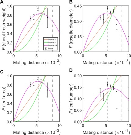
The mean and SE of F are shown by black squares and associated error bars, respectively. The fitted D-F curves under different models are shown in different colors. Statistics of model fitting are provided in Table 2. Nucleotide diversity (π) and maximal intraspecific genetic distance observed (D_max) are indicated by vertical dotted and dashed lines, respectively.

Model III is favored in mouse

We also expanded our analysis to animals by analyzing 28 crosses of the mouse Mus musculus (19). Two fitness-related traits, body weight and reproductive rate, were examined (see Materials and Methods). For each trait, model III fits the data significantly better than the other two models (table S4), and a humped curve is observed under model III (fig. S3). The OMDs for the two traits are 5.1 × 10⁻³ and 6.6 × 10⁻³, respectively (table S4), between π (3.3 × 10⁻³) and D_max (9.3 × 10⁻³) of the species (see Materials and Methods).

Statistical support for model III is robust

In all three species, we found model III to be superior to the other two models by various statistical indices. To further examine whether model III is also an adequate model in explaining the data, we conducted a test of model heteroscedasticity. We focused on yeast and Arabidopsis, because the mouse data are too small to be statistically meaningful in this test. We found that the predicted F ($\widehat{{\mathit{F}}_{\mathit{k}}}$, k refers to the kth data point) from model III is correlated with neither the regression residual ${\mathrm{\varepsilon }}_{\mathit{k}}={\mathit{F}}_{\mathit{k}}-\widehat{{\mathit{F}}_{\mathit{k}}}$ (table S5) nor | ɛ_k| (P > 0.3), indicating that model III describes the relationship between D and F in the entire range of the data equally well and is not missing any trend in the data. By contrast, $\widehat{{\mathit{F}}_{\mathit{k}}}$ predicted from the other two models is almost always significantly negatively correlated with ɛ_k (table S5), suggesting that these two models miss certain trends in the data.

We used fixed-intercept models in our analyses because the biology dictates that F should be 0 when D is 0. Notwithstanding, we found model III to be superior to the other two models in all three species even when the intercept is not fixed and the point of (D = 0, F = 0) is simply treated as a datum in the analysis (table S6). In other words, among the three modified models, F = aD + c (model I), F = bD² + c (model II), and F = aD + bD² + c (model III), model III is still best supported by the data.

We showed that R² is generally much greater for model III than for the other two models. However, because model III has one more parameter than each of the other two models, their R² values are not directly comparable. We therefore calculated R² of F = aD^b (model IV) to allow directly comparing R² between models III and IV. Note that, despite the elevated flexibility over models I and II, model IV still allows only a monotonic relation between D and F. In the yeast dataset (14), model IV has an R² = 0.37, while model III has a much higher R² of 0.85. Similarly, model III has a much higher R² for all four traits (0.54, 0.44, 0.63, and 0.39) than model IV (0.15, 0.00, 0.01, and 0.19) in Arabidopsis. For mice, model III has R² = 0.95 and 0.51 for body weight and reproductive rate, respectively, while model IV has R² = 0.63 and 0.55, respectively. Therefore, except for the mouse reproductive rate, model III shows a much higher R² than model IV. Hence, model III is generally superior to model IV.

DISCUSSION

In summary, we detected the long anticipated hump-shaped relationship between D and F in each of the three model organisms examined, which represent three major eukaryotic lineages. Our finding is also robust to the specific trait, environment, and method of analysis. Our success has a number of contributing factors, the lack of which likely explains why a humped relationship was not previously observed. First, the range of D in the data should encompass the OMD; otherwise, the humped relationship is easily missed. Second, an accurate measure of D, ideally based on genome sequences, is necessary for detecting the hump. Third, the variance of F among crosses at a given D is usually large, requiring the use of many crosses to obtain reliable estimates. Fourth, crossing homozygotes simplifies the expectation and reduces the variance of F. Last but not least, having a mathematical model describing the theoretically expected relationship between D and F helps verify their relation. For instance, without such a model, authors of the original Arabidopsis study incorrectly concluded that F is independent of D on the basis of no significant linear correlation (13).

That model III surpasses the other models in explaining almost all datasets analyzed has several biological implications. First, it is currently unclear whether heterosis is caused by dominance, overdominance, or positive intergenic epistasis (4). While our results do not confirm or refute the roles of overdominance and positive intergenic epistasis, they firmly establish the general contribution of dominance, because a, the coefficient of the linear term in model III, is found to be positive in all three species examined. Second, b, the coefficient of the quadratic term, reflects the sum of the incompatibility effect and the heterotic effect other than dominance. Because b is found to be negative while the heterotic effect is, by definition, nonnegative, the incompatibility effect must be negative. This result, again found in all three species studied, echoes the finding in fruitflies (20) and tomatoes (21) that the number of incompatibilities between two genotypes increases in proportion to D² and further demonstrates that fitness-related phenotypic effects of incompatibility also increase in proportion to D². Third, while the fly and tomato studies used only interspecific crosses (20, 21), our crosses are all intraspecific. Hence, even within species, genetic incompatibility, which could be a result of genetic drift and/or local adaptation, not only exists (22) but also snowballs. Fourth, the net effect of heterosis and incompatibility on hybrid performance rises as D increases from 0 to the OMD, but retreats when D further increases, and is expected to eventually become negative when D exceeds twice the OMD. Because nonrandom mating and population structure is widespread in nature, the accumulation of genetic incompatibility within species could generate a selective pressure against interbreeding between distantly related conspecifics and initiate speciation. The importance of this process in nature may be tested by examining how often the OMD is below D_max, because speciation could not be triggered by intraspecific incompatibilities if OMD > D_max. When OMD < D_max, as found in all three species examined, a low OMD may predict a high rate of speciation, and studying the incompatibilities between distantly related conspecifics may shed light on the genetic basis of incipient speciation. Note that the OMD can be recognized even if it exceeds D_max because relevant studies often include interspecific crosses (12). Note that several earlier studies examined plant optimal geographical distances in artificial outcrossing and found them to be extremely small (5 to 20 m) (23–25). This is probably because the plant performances were measured in local environments rather than in a common garden. Consequently, the performance differences may not be entirely genetic.

Our findings also have implications for animal and plant breeding. To boost the hybrid performance, one should not only take the advantage of heterosis but also minimize the negative impact of incompatibility. Hence, the best mating distance should be close to the estimated OMD rather than to D_max, as one might think without considering the impact of intraspecific genetic incompatibility. Further, because we found that the OMDs of multiple fitness-related traits in a given species tend to be similar, using mating distances close to the OMD will likely optimize a suite of fitness-related traits. One potential reason for the similar OMDs of different traits is mutational pleiotropy (26). To explore this possibility, we correlated trait values among all strains in our data. In yeast, the average Pearson’s r between growth rate in one environment and those in the other 10 environments ranges from 0.04 to 0.53. In Arabidopsis, Pearson’s r between two traits among all strains ranges from 0.05 (insignificant) to 0.85 (significant). The correlation between mouse weight and reproductive rate is high in males (r = 0.81, P = 1.2 × 10⁻¹⁰) but moderate in females (r = 0.32, P = 0.012). Therefore, pleiotropy is probably one of several reasons for similar OMDs among traits.

In conservation biology, it is well appreciated that too small of a D is harmful due to inbreeding depression (27). Because all parents are homozygotes in the crosses analyzed here, both the observation of positive F and that of a rise in F with D when D < OMD demonstrate inbreeding depression. Many studies showed that too large of a D can cause outbreeding depression and is also undesirable (28). Our results suggest that applying the OMD in managing conservation may be most effective. In all three species studied, the OMDs of most traits are similar to or greater than π but smaller than D_max. This pattern, if further confirmed in additional lineages, suggests the general strategy of using mating distances slightly higher than π to minimize both inbreeding and outbreeding depressions when the OMD is unknown.

MATERIALS AND METHODS

Genetic distance and phenotypic data

The S. cerevisiae data were primarily acquired from two sources. Our analysis focused on the data of Plech et al. (14), which contained all 231 pairwise mating from 22 haploid parental strains. The range of genetic distance covered in Plech et al.’s data is larger than that in Zörgö et al.’s yeast data (17). Plech et al.’s data included maximum growth rates for the homozygous diploid parents and hybrids in 11 liquid media. They are YPD (nutrient rich with 2% glucose) at 30°C, Gal (nutrient rich with 2% galactose) at 30°C, YPG (nutrient rich with 3% glycerol) at 30°C, SD (synthetic medium with 2% glucose supplemented with uracil) at 30°C, Y20 (YPD at 20°C), Y35 (YPD at 35°C), and five YPD-based media at 30°C with additional chemicals indicated: Ben [benomyl (40 μg/ml)], DM (6% dimethyl sulfoxide), Na (2% NaCl), Sal (2% salicylate), and Zn [ZnSO₄ (0.5 mg/ml)]. Mating distances were from Liti et al. (29), calculated from 235,127 SNPs. We did not use the distances from a more recent study that sequenced yeast genomes to a higher coverage, due to its underestimation of distances by including gaps and missing data in the genome size (30), but because Liti et al. did not calculate the genome-wide π and included fewer strains than the more recent study (30), we extrapolate π and D_max from the more recent study. Specifically, we regressed the distances between the two studies using all shared strains between them. On the basis of the linear regression (r = 0.99, P = 5.9 × 10⁻²⁰⁰), we converted π and D_max from the more recent study by dividing them by 0.69.

We also analyzed Zörgö et al.’s yeast data, which included 28 pairwise crosses among eight strains and measures of parent and hybrid phenotypes in growth rate, lag time, and yield in 56 environments (17). Note that because a greater lag time indicates a lower fitness, we used negative lag time as a fitness-related trait. We analyzed the mean F from all environments to increase the accuracy of F estimates because of the relatively small number of crosses performed.

We examined Bernardes et al.’s data from 27 crosses of S. paradoxus (18). The genetic distance and competitive fitness data were acquired from their table S1. We converted their logarithm of competitive fitness back to competitive fitness, but this conversion did not alter the result.

We acquired the A. thaliana phenotypic and genetic distance data from Yang et al. (13). There were 200 intraspecific hybrids generated by crossing 200 A. thaliana accessions with one common maternal accession. The hybrids and their parents were measured for four traits at 14 days after sowing: shoot fresh weight, rosette diameter, leaf area, and leaf number. The genomes of 191 parental accessions had been sequenced (13). In the original study (13), the genetic distance between parents was calculated by PLINK based on 722,000 SNPs. A. thaliana has a reference genome of ~116.8 Mb. Using genome sequences, we calculated that the genome-wide per nucleotide distance between Col-0 and the commonly used Ler-1 equals 5.4 × 10⁻³. Using this information allowed us to convert per SNP distance in the original study to per nucleotide distance for all pairs of accessions. We included all 191 hybrids with available per nucleotide genetic distances in our analysis. Genome-wide nucleotide diversity was estimated using the results of Nordborg et al. (31). D_max was calculated from the maximum distance of 10,000 random pairs of strains from the 1135 genome-sequenced strains provided by the 1001 Arabidopsis Genome Project. Sampling 20,000 random pairs of strains did not increase D_max. All Arabidopsis whole-genome variant call format (VCF) files were downloaded from http://1001genomes.org/data-center.html.

The phenotypic data of M. musculus were acquired from Philip et al. (19). We used body weight and reproductive rate (first litter size divided by the time from first mating to first litter) as fitness-related traits (32). Because of the scarcity of data, we did not separate male and female hybrid animals in our analysis. We downloaded the whole-genome SNP data generated by Yalcin et al. (33) for the eight parental strains (ftp://ftp-mouse.sanger.ac.uk/current_snps/strain_specific_vcfs/) and estimated D by the number of SNPs per site between parental genomes. We used a window size of D = 10⁻³ to bin the crosses. Because the D values of the 28 crosses cluster into four small groups, using a smaller window size such as D = 0.5 × 10⁻³ does not give more useful bins. Mouse has a π of 3.3 × 10⁻³ (34), and we estimated that D_max = 9.3 × 10⁻³ using the genome sequences of the two most diverged subspecies of M. musculus, CAST/EiJ and PWK/PhJ (35).

Causes of heterosis and genetic incompatibility

Heterosis in F1 hybrids arises from genetic interactions between the paternal and maternal alleles of the same loci (via dominance and overdominance) and/or different loci (via positive intergenic epistasis) (4). Genetic incompatibility similarly originates from allelic interactions at the same loci (via underdominance) and/or different loci (via negative intergenic epistasis). At any locus, if the paternal and maternal alleles differ, then either both of them are derived from their common ancestral allele at their coalescence or only one of them is derived whereas the other is ancestral.

Because fitter alleles tend to be partially or completely dominant over less fit alleles (36), when homozygous individuals from different populations hybridize, dominance can cause the hybrid to outperform the average of the two parents and result in heterosis. Because the occurrence of heterosis by dominance requires a change from the ancestral state in only one parent, it should rise in proportion to mating distance D. Overdominance, underdominance, positive intergenic epistasis, and negative intergenic epistasis can obviously occur in the hybrid between two derived alleles that are respectively homozygous in the two parents. Should overdominance between an ancestral and a derived allele occur, the derived allele will likely stay in the heterozygous state in one population; hence, heterosis is unlikely to occur upon hybridization. Similarly, should positive intergenic epistasis exist between an ancestral and a derived allele, this positive effect is already seen in one parent and thus is not heterotic. Should underdominance or negative intergenic epistasis occur between an ancestral and a derived allele, the derived allele will likely be selectively removed from the population and therefore is unlikely to contribute to genetic incompatibility between the two parents. Therefore, the effects from overdominance, underdominance, positive intergenic epistasis, and negative intergenic epistasis should most likely increase in proportion to D².

Parameter estimation

All calculations were performed using MATLAB. The coefficient of determination (R²) used here is defined as R² = 1 − $\frac{\sum {({\mathit{y}}_{\mathit{k}}-\widehat{{\mathit{y}}_{\mathit{k}}})}^2}{\sum {({\mathit{y}}_{\mathit{k}}-\overline{\mathit{y}})}^2}$, where y_k is the kth observation of the variable Y, $\widehat{{\mathit{y}}_{\mathit{k}}}$ is the corresponding prediction by a model, and $\overline{\mathit{y}}$ is the overall mean of Y. This definition of R² is the most commonly used, recommended even for non-intercept models (37). It gives the intuitive interpretation across a wide variety of contexts in terms of the proportion of total variation of Y (around its mean $\overline{\mathit{y}}$) that is explained by the fitted model (37). Note that R² becomes negative when the fitted model is worse than the mean of Y in explaining the variation of Y. We used the function “lsqcurvefit” to perform least-squares estimations of model parameters. We then used the estimated parameters to compute R² and conduct LRTs. Twice the difference in ln(likelihood) between model III and model I (or II), or 2ΔlnL, equals Nln(SSE_{I or II}/SSE_III), where N is the number of (binned) data points in the regression and the sum of squared errors of prediction SSE = ${\sum }_{\mathit{k}=1}^{\mathit{N}}{({\mathit{y}}_{\mathit{k}}-\widehat{{\mathit{y}}_{\mathit{k}}})}^2$. The above formula of 2ΔlnL is derived as follows. The likelihood of the linear regression model between the independent variable X and dependent variable Y is L(β, σ², Y, X) = (2πσ²)^−N/2exp[$\frac{-1}{2{\mathrm{\sigma }}^2}{\sum }_{\mathit{k}=1}^{\mathit{N}}{({\mathit{y}}_{\mathit{k}}{-\mathrm{\beta }\mathit{x}}_{\mathit{k}})}^2$], where β is the vector of parameters in the model and errors follow a Gaussian distribution with the mean = 0 and variance = σ². Hence, lnL(β, σ², Y, X) = $-\frac{\mathit{N}}{2}\text{ln}(2\mathrm{\pi })-\frac{\mathit{N}}{2}\text{ln}({\mathrm{\sigma }}^2)-\frac{1}{2{\mathrm{\sigma }}^2}{\sum }_{\mathit{k}=1}^{\mathit{N}}{({\mathit{y}}_{\mathit{k}}{-\mathrm{\beta }\mathit{x}}_{\mathit{k}})}^2$. It can be shown that lnL(β, σ², Y, X) reaches the maximum when σ² = $\widehat{{\mathrm{\sigma }}^2}=\frac{1}{\mathit{N}}{\sum }_{\mathit{k}=1}^{\mathit{N}}{({\mathit{y}}_{\mathit{k}}-\widehat{\mathrm{\beta }}{\mathit{x}}_{\mathit{k}})}^2$, where $\widehat{\mathrm{\beta }}$ is the maximum likelihood estimate of β. The maximized lnL(β, σ², Y, X) equals $-\frac{\mathit{N}}{2}\text{ln}(2\mathrm{\pi })+\frac{\mathit{N}}{2}\text{ln}\mathit{N}-\frac{\mathit{N}}{2}\text{ln}{\sum }_{\mathit{k}=1}^{\mathit{N}}{({\mathit{y}}_{\mathit{k}}-\widehat{\mathrm{\beta }}{\mathit{x}}_{\mathit{k}})}^2-\frac{\mathit{N}}{2}$ = $-\frac{\mathit{N}}{2}\text{ln}(2\mathrm{\pi })+\frac{\mathit{N}}{2}\text{ln}\mathit{N}-\frac{\mathit{N}}{2}-\frac{\mathit{N}}{2}\text{ln}(\text{SSE})$. For a given dataset, the first three terms in the above formula are constant and are cancelled out when two models are compared. Hence, 2ΔlnL between model III and model I (or II) is NlnSSE_{I or II} − NlnSSE_III = Nln(SSE_{I or II}/SSE_III). P values of LRTs are determined by chi-square tests with 1 df using the MATLAB-embedded function “chi2cdf.” We computed the OMD in model III to be −0.5a/b, where a and b are parameters of the model estimated using least-squares regression. The confidence interval of OMD was estimated by a bootstrap method. Specifically, we randomly sampled from all crosses with replacement the same number of crosses as in the original data and then estimated the OMD from the sampled crosses. We repeated this process 1000 times to acquire the 95% confidence interval of the OMD. In our model fitting, mean D of a bin is the independent variable, whereas mean F of a bin is the dependent variable.

We also performed WLS regression using 1/SE² as the weight, where SE is the standard error of the mean F of a bin; that is, bins with larger estimation errors of mean F carry lower weights in model fitting. We computed R² from the WLS regression in the weighted space (R²_WLS) [eq. 4 in Willett and Singer (38)] and the corresponding optimal mating distance (OMD_WLS).

Although better parent heterosis (BPH) (17), which describes the phenotypic difference between the hybrid and the better parent, is also commonly used to study heterosis, there is no clear theoretical relationship between D and BPH. Hence, we focused on F, which is also known as the heterosis coefficient (17). Throughout this study, we examined the impact of the genetic distance between two individuals on the performance of their offspring (i.e., F1) and identified the OMD, because of the availability of F1 phenotypes in large numbers of crosses. In theory, it is also possible to study the impact of the genetic distance between two individuals on the performance of their grandchildren (i.e., F2 generated by random mating among F1 individuals) (15). OMD for F2 is presumably smaller than that for F1, because recessive genetic incompatibilities masked in F1 may be exposed in F2. It will be interesting to test this prediction when F2 phenotypes from large numbers of crosses become available.

SUPPLEMENTARY MATERIALS

Supplementary material for this article is available at http://advances.sciencemag.org/cgi/content/full/4/11/eaau5518/DC1

Fig. S1. Hump-shaped relationship between S. cerevisiae mating distance (D) and hybrid performance (F) measured by maximum growth rate in the Ben medium.

Fig. S2. Hump-shaped relationship between S. cerevisiae mating distance (D) and hybrid performance (F) in (A) maximum growth rate, (B) negative lag time, and (C) proliferative efficiency averaged across 56 environments.

Fig. S3. Hump-shaped relationship between M. musculus mating distance (D) and hybrid performance (F) in (A) body weight and (B) reproductive rate.

Table S1. Fitting of the three models to the S. cerevisiae data (averaged across 11 environments) using alternative window sizes.

Table S2. Fitting of the three models to Zörgö et al.’s yeast data

Table S3. Fitting of the three models to the A. thaliana data using alternative window sizes.

Table S4. Fitting of the three models to the M. musculus data.

Table S5. Test of heteroscedasticity of the three models in S. cerevisiae and A. thaliana.

Table S6. Model fitting without a fixed intercept.

REFERENCES AND NOTES

- 1.C. Darwin, The Effects of Cross- and Self-fertilisation in the Vegetable Kingdom (John Murray, 1876). [Google Scholar]
- 2.Shull G. H., The composition of a field of maize. Am. Breed. Assn. Rep. 4, 296–301 (1908). [Google Scholar]
- 3.E. M. East, Inbreeding in corn, in Reports of the Connecticut Agricultural Experiment Station for Years 1907–1908 (Connecticut Agricultural Experiment Station, 1908), pp. 419–428. [Google Scholar]
- 4.Lippman Z. B., Zamir D., Heterosis: Revisiting the magic. Trends Genet. 23, 60–66 (2007). [DOI] [PubMed] [Google Scholar]
- 5.T. Dobzhansky, Genetics and the Origin of Species (Columbia Univ. Press, 1937). [Google Scholar]
- 6.Muller H. J., Isolating mechanisms, evolution and temperature. Biol. Symp. 6, 71–125 (1942). [Google Scholar]
- 7.J. A. Coyne, H. A. Orr, Speciation (Sinauer Associates, 2004). [Google Scholar]
- 8.Bateson P., Sexual imprinting and optimal outbreeding. Nature 273, 659–660 (1978). [DOI] [PubMed] [Google Scholar]
- 9.Stelkens R. B., Pompini M., Wedekind C., Testing the effects of genetic crossing distance on embryo survival within a metapopulation of brown trout (Salmo trutta). Conserv. Genet. 15, 375–386 (2014). [Google Scholar]
- 10.Robinson S. P., Kennington W. J., Simmons L. W., No evidence for optimal fitness at intermediate levels of inbreeding in Drosophila melanogaster. Biol. J. Linn. Soc. 98, 501–510 (2009). [Google Scholar]
- 11.Moll R. H., Lonnquist J. H., Fortuno J. V., Johnson E. C., The relationship of heterosis and genetic divergence in maize. Genetics 52, 139–144 (1965). [DOI] [PMC free article] [PubMed] [Google Scholar]
- 12.Willi Y., Van Buskirk J., Genomic compatibility occurs over a wide range of parental genetic similarity in an outcrossing plant. Proc. Biol. Sci. 272, 1333–1338 (2005). [DOI] [PMC free article] [PubMed] [Google Scholar]
- 13.Yang M., Wang X., Ren D., Huang H., Xu M., He G., Deng X. W., Genomic architecture of biomass heterosis in Arabidopsis. Proc. Natl. Acad. Sci. U.S.A. 114, 8101–8106 (2017). [DOI] [PMC free article] [PubMed] [Google Scholar]
- 14.Plech M., de Visser J. A. G. M., Korona R., Heterosis is prevalent among domesticated but not wild strains of Saccharomyces cerevisiae. G3 4, 315–323 (2014). [DOI] [PMC free article] [PubMed] [Google Scholar]
- 15.Lynch M., The genetic interpretation of inbreeding depression and outbreeding depression. Evolution 45, 622–629 (1991). [DOI] [PubMed] [Google Scholar]
- 16.Edmands S., Does parental divergence predict reproductive compatibility? Trends Ecol. Evol. 17, 520–527 (2002). [Google Scholar]
- 17.Zörgö E., Gjuvsland A., Cubillos F. A., Louis E. J., Liti G., Blomberg A., Omholt S. W., Warringer J., Life history shapes trait heredity by accumulation of loss-of-function alleles in yeast. Mol. Biol. Evol. 29, 1781–1789 (2012). [DOI] [PubMed] [Google Scholar]
- 18.Bernardes J. P., Stelkens R. B., Greig D., Heterosis in hybrids within and between yeast species. J. Evol. Biol. 30, 538–548 (2017). [DOI] [PubMed] [Google Scholar]
- 19.Philip V. M., Sokoloff G., Ackert-Bicknell C. L., Striz M., Branstetter L., Beckmann M. A., Spence J. S., Jackson B. L., Galloway L. D., Barker P., Wymore A. M., Hunsicker P. R., Durtschi D. C., Shaw G. S., Shinpock S., Manly K. F., Miller D. R., Donohue K. D., Culiat C. T., Churchill G. A., Lariviere W. R., Palmer A. A., O’Hara B. F., Voy B. H., Chesler E. J., Genetic analysis in the Collaborative Cross breeding population. Genome Res. 21, 1223–1238 (2011). [DOI] [PMC free article] [PubMed] [Google Scholar]
- 20.Matute D. R., Butler I. A., Turissini D. A., Coyne J. A., A test of the snowball theory for the rate of evolution of hybrid incompatibilities. Science 329, 1518–1521 (2010). [DOI] [PubMed] [Google Scholar]
- 21.Moyle L. C., Nakazato T., Hybrid incompatibility “snowballs” between Solanum species. Science 329, 1521–1523 (2010). [DOI] [PubMed] [Google Scholar]
- 22.Corbett-Detig R. B., Zhou J., Clark A. G., Hartl D. L., Ayroles J. F., Genetic incompatibilities are widespread within species. Nature 504, 135–137 (2013). [DOI] [PMC free article] [PubMed] [Google Scholar]
- 23.Price M. V., Waser N. M., Pollen dispersal and optimal outcrossing in Delphinium nelsoni. Nature 277, 294–297 (1979). [Google Scholar]
- 24.Campbell D. R., Waser N. M., The evolution of plant mating systems: Multilocus simulations of pollen dispersal. Am. Nat. 129, 593–609 (1987). [Google Scholar]
- 25.Schierup M. H., Christiansen F. B., Inbreeding depression and outbreeding depression in plants. Heredity 77, 461–468 (1996). [Google Scholar]
- 26.Wagner G. P., Zhang J., The pleiotropic structure of the genotype-phenotype map: The evolvability of complex organisms. Nat. Rev. Genet. 12, 204–213 (2011). [DOI] [PubMed] [Google Scholar]
- 27.Hedrick P. W., Kalinowski S. T., Inbreeding depression in conservation biology. Annu. Rev. Ecol. Syst. 31, 139–162 (2000). [Google Scholar]
- 28.Edmands S., Between a rock and a hard place: Evaluating the relative risks of inbreeding and outbreeding for conservation and management. Mol. Ecol. 16, 463–475 (2007). [DOI] [PubMed] [Google Scholar]
- 29.Liti G., Carter D. M., Moses A. M., Warringer J., Parts L., James S. A., Davey R. P., Roberts I. N., Burt A., Koufopanou V., Tsai I. J., Bergman C. M., Bensasson D., O’Kelly M. J. T., van Oudenaarden A., Barton D. B. H., Bailes E., Nguyen A. N., Jones M., Quail M. A., Goodhead I., Sims S., Smith F., Blomberg A., Durbin R., Louis E. J., Population genomics of domestic and wild yeasts. Nature 458, 337–341 (2009). [DOI] [PMC free article] [PubMed] [Google Scholar]
- 30.Maclean C. J., Metzger B. P. H., Yang J. R., Ho W.-C., Moyers B., Zhang J., Deciphering the genic basis of yeast fitness variation by simultaneous forward and reverse genetics. Mol. Biol. Evol. 34, 2486–2502 (2017). [DOI] [PubMed] [Google Scholar]
- 31.Nordborg M., Hu T. T., Ishino Y., Jhaveri J., Toomajian C., Zheng H., Bakker E., Calabrese P., Gladstone J., Goyal R., Jakobsson M., Kim S., Morozov Y., Padhukasahasram B., Plagnol V., Rosenberg N. A., Shah C., Wall J. D., Wang J., Zhao K., Kalbfleisch T., Schulz V., Kreitman M., Bergelson J., The pattern of polymorphism in Arabidopsis thaliana. PLOS Biol. 3, e196 (2005). [DOI] [PMC free article] [PubMed] [Google Scholar]
- 32.K. Flurkey, J. M. Currer, The Jackson Laboratory Handbook on Genetically Standardized Mice (Jackson Laboratory, 2009). [Google Scholar]
- 33.Yalcin B., Wong K., Agam A., Goodson M., Keane T. M., Gan X., Nellåker C., Goodstadt L., Nicod J., Bhomra A., Hernandez-Pliego P., Whitley H., Cleak J., Dutton R., Janowitz D., Mott R., Adams D. J., Flint J., Sequence-based characterization of structural variation in the mouse genome. Nature 477, 326–329 (2011). [DOI] [PMC free article] [PubMed] [Google Scholar]
- 34.Frazer K. A., Eskin E., Kang H. M., Bogue M. A., Hinds D. A., Beilharz E. J., Gupta R. V., Montgomery J., Morenzoni M. M., Nilsen G. B., Pethiyagoda C. L., Stuve L. L., Johnson F. M., Daly M. J., Wade C. M., Cox D. R., A sequence-based variation map of 8.27 million SNPs in inbred mouse strains. Nature 448, 1050–1053 (2007). [DOI] [PubMed] [Google Scholar]
- 35.Goios A., Pereira L., Bogue M., Macaulay V., Amorim A., mtDNA phylogeny and evolution of laboratory mouse strains. Genome Res. 17, 293–298 (2007). [DOI] [PMC free article] [PubMed] [Google Scholar]
- 36.Fisher R. A., The possible modification of the response of the wild type to recurrent mutations. Am. Nat. 62, 115–126 (1928). [Google Scholar]
- 37.Kvålseth T. O., Cautionary note about R2. Am. Stat. 39, 279–285 (1985). [Google Scholar]
- 38.Willett J. B., Singer J. D., Another cautionary note about R2: Its use in weighted least-squares regression-analysis. Am. Stat. 42, 236–238 (1988). [Google Scholar]
Associated Data
This section collects any data citations, data availability statements, or supplementary materials included in this article.