Solving stereo transparency with an extended coarse-to-fine disparity energy model

Abstract

Modeling stereo transparency with physiologically plausible mechanisms is challenging because in such frameworks, large receptive fields mix up overlapping disparities whereas small receptive fields can reliably compute only small disparities. It seems necessary to combine information across scales. A coarse-to-fine disparity energy model, with both position- and phase-shift receptive fields, has already been proposed. However, because each scale decodes only one disparity for each location and uses the decoded disparity to select cells at the next scale, this model cannot represent overlapping surfaces at different depths. We have now extended the model to solve stereo transparency. First, we introduce multiplicative connections from cells at one scale to the next to implement coarse-to-fine computation. The connection is the strongest when the pre-synaptic cell’s preferred disparity matches the post-synaptic cell’s position-shift parameter, encouraging the next scale to encode residual disparities with the more reliable phase-shift mechanism. This modification not only eliminates the artificial decoding and selection steps of the original model but also enables maintenance of complete population responses throughout the coarse-to-fine process. Second, because of the above modification, explicit decoding is no longer necessary but rather is for visualization only. We use a simple threshold criterion to decode multiple disparities from population energy responses, instead of a single disparity in the original model. We demonstrate our model via simulations on a variety of transparent and non-transparent stereograms. The model also reproduces psychophysically observed disparity interactions (averaging, thickening, attraction, and repulsion) as the depth separation between two overlapping planes varies.

1. Introduction

We can see overlapping surfaces at different depths in transparent random-dot stereograms (Julesz, 1971; Prazdny, 1985). Computationally, however, this so-called stereo transparency problem is difficult to solve with physiologically plausible methods such as the disparity energy model (Ohzawa et al., 1990; Qian, 1994, 1997). On one hand, cells with large receptive fields (RFs) cover dots carrying different disparities, mixing them in the cells’ responses. On the other hand, cells with small RFs can reliably compute only small disparities; this is true even for position-shift RFs (Chen and Qian 2004, also see Discussions). Consequently, a model has to use RFs that are much smaller than distances between adjacent dots in a stereogream but much larger than the disparities involved. This requires that the disparities be much smaller than the distances between adjacent dots. The transparent random-dot stereogram in Fig. 1, for example, violates this requirement, yet we can still perceive two transparent surfaces.

Figure 1:

Chen and Qian (2004)’s model applied to a transparent random-dot stereogram with two overlapping planes of 3 and −2 pixels of disparities, respectively. The model can decode only one disparity at each position, resulting in a patch-wise map of the two actual disparities.

Extant models of stereo transparency often include non-biological procedures to get around the above problem. For example, a large class of models follows Marr and Poggio (1976) by starting with a compatibility map that contains all possible matches between features in the two eyes, and then introducing constraints to eliminate false matches (Prazdny, 1985; Pollard et al., 1985; Qian and Sejnowski, 1989; Zhaoping, 2002). Such models are non-physiological because they do not use any reasonable RFs, and each unit of a compatibility map responds to only one potential match (Qian, 1997). If the compatibility map is replaced by disparity energy responses produced by realistic RFs, then the Marr-Poggio style constraints cannot be applied because the energy responses are broadly distributed with multiple peaks (Qian, 1994; Chen and Qian, 2004; Assee and Qian, 2007).

In this study, we solve stereo transparency in the framework of the disparity energy model (Ohzawa et al., 1990; Qian, 1994). Since, as mentioned above, a single RF scale appears to be inadequate, it seems natural to combine information across scales. Intuitively, although a large scale may average overlapping stimulus disparities, the average could still be a good starting point for smaller scales to resolve multiple disparities. Conversely, a small scale alone cannot reliably compute large disparities but can use larger scales’ guidance to offset stimulus disparities with the position-shift component of RFs and compute the residual disparity of each surface with the more reliable phase-shift component (Chen and Qian, 2004). A coarse-to-fine version of the disparity energy model, with both position- and phase-shift RFs, has already been proposed (Chen and Qian, 2004) and successfully applied to non-transparent stereograms. However, each scale of this model decodes only a single disparity for each location and uses the decoded disparity to select cells in the next scale. Consequently, it cannot represent multiple, transparent surfaces at a location. We have now extended this model to solve stereo transparency and at the same time to make it more biologically plausible by eliminating explicit decoding and selection during computation. Preliminary results were presented in abstract form (Li and Qian, 2014).

2. Method

2.1. Coarse-to-fine disparity energy model

We first briefly describe Chen and Qian’s coarse-to-fine disparity energy model and then explain our extensions. The model employs hybrid binocular cells with both position and phase shifts between the two eyes’ RFs (Zhu and Qian, 1996; Ohzawa et al., 1997; Anzai et al., 1997, 1999; Livingstone and Tsao, 1999; Prince et al., 2002). For convenience, we first define Gabor function with orientation θ (measured from horizontal) as:

$$G(x,y;\sigma ,\theta ,\varphi )=\frac{1}{2\pi {\sigma }_{\perp }{\sigma }_{\parallel }}\text{exp}\left(-\frac{{x^{\prime }}^2}{2{\sigma }_{\perp }^2}-\frac{{y^{\prime }}^2}{2{\sigma }_{\parallel }^2}\right)\text{cos}\left(\omega x^{\prime }-\varphi \right)$$ (1)

where (x′, y′) is (x, y) rotated by angle θ, σ_⊥ ≡ σ characterizes the spatial scale, σ_∥ = kσ_⊥ determines RF aspect ratio k (set to 2 in our simulations), and $\omega =\frac{\pi }{\sigma }$ is the preferred spatial frequency. We keep $\frac{{\sigma }_{\parallel }}{{\sigma }_{\perp }}$ and ωσ constant across scales to ensure scale-invariant RF shapes.

The left and right RFs of a simple cell is then given by:

$$F_{\text{L}1}\left(x,y;\sigma ,\theta ,d,\mathrm{\Delta }\varphi \right)=G(x-\frac{d}{2},y;\sigma ,\theta ,\frac{\mathrm{\Delta }\varphi }{2})$$ (2)

$$F_{\text{R}1}\left(x,y;\sigma ,\theta ,d,\mathrm{\Delta }\varphi \right)=G(x+\frac{d}{2},y;\sigma ,\theta ,-\frac{\mathrm{\Delta }\varphi }{2})$$ (3)

where d and Δϕ are the position- and phase-shift parameters, respectively. Another simple cell forming a quadrature pair with this cell has RFs given by:

$$F_{\text{L}2}\left(x,y;\sigma ,\theta ,d,\mathrm{\Delta }\varphi \right)=G(x-\frac{d}{2},y;\sigma ,\theta ,\frac{\mathrm{\Delta }\varphi }{2}-\frac{\pi }{2})$$ (4)

$$F_{\text{R}2}\left(x,y;\sigma ,\theta ,d,\mathrm{\Delta }\varphi \right)=G(x+\frac{d}{2},y;\sigma ,\theta ,-\frac{\mathrm{\Delta }\varphi }{2}-\frac{\pi }{2})$$ (5)

The responses of these simple cells at position (x, y) to the left and right images, I_L (x, y) and I_R (x, y), are:

$$\begin{gathered} r_1(x,y;\sigma ,\theta ,d,\mathrm{\Delta }\varphi )=\int \text{d}{x}^{\prime }\text{d}{y}^{\prime }{I}_{\text{L}}(x+x^{\prime },y+y^{\prime })F_{\text{L}1}(x^{\prime },y^{\prime }) \\ +\int \text{d}{x}^{\prime }\text{d}{y}^{\prime }{I}_{\text{R}}(x+x^{\prime },y+y^{\prime })F_{\text{R}1}(x^{\prime },y^{\prime }) \end{gathered}$$ (6)

$$\begin{gathered} r_2(x,y;\sigma ,\theta ,d,\mathrm{\Delta }\varphi )=\int \text{d}{x}^{\prime }\text{d}{y}^{\prime }{I}_{\text{L}}(x+x^{\prime },y+y^{\prime })F_{\text{L}2}(x^{\prime },y^{\prime }) \\ +\int \text{d}{x}^{\prime }\text{d}{y}^{\prime }{I}_{\text{R}}(x+x^{\prime },y+y^{\prime })F_{\text{R}2}(x^{\prime },y^{\prime }) \end{gathered}$$ (7)

The energy response of the complex cell receiving inputs from this quadrature pair of simple cells is then:

$$r_{\text{c}}(x,y;\sigma ,\theta ,d,\mathrm{\Delta }\varphi )=r_1^2(x,y;\sigma ,\theta ,d,\mathrm{\Delta }\varphi )+r_2^2(x,y;\sigma ,\theta ,d,\mathrm{\Delta }\varphi )$$ (8)

For a stimulus with disparity D evenly divided between the two eyes, the response is approximately (when $\left|D-d\right|\ll \frac{{\sigma }_{\perp }}{\text{sin}\theta }$, see Appendix)

$$r_{\text{c}}\approx 4A^2{\text{cos}}^2\left(\frac{\omega }{2}\left[D-(d+\frac{\mathrm{\Delta }\varphi }{\omega \text{sin}\theta })\right]\right)$$ (9)

where A is the Fourier amplitude of local image patch. Thus, the cell’s preferred disparity is approximately:

$$D^{*}\approx d+\frac{\mathrm{\Delta }\varphi }{\omega \text{sin}\theta }$$ (10)

To improve performance, Chen and Qian pooled energy responses across orientation and space according to:

$$r(d,\mathrm{\Delta }\varphi ;x,y,\sigma )=\sum _{i=1}^5{r}_{\text{c}}(x,y;\sigma ,{\theta }_i,d,\mathrm{\Delta }{\varphi }_i)+F_{\text{sp}}(x,y;\sigma )$$ (11)

where the 5 orientations are:

$${\theta }_i=\frac{i\pi }{6}(i=1,2,\dots ,5),$$ (12)

Δϕ_i = Δϕ sin θ_i ensures that the pooled cells of different orientations have the same preferred disparity, and the spatial pooling kernel for scale σ is

$$F_{\text{sp}}(x,y;\sigma )=\frac{1}{2\pi {\sigma }^2}\text{exp}\left(-\frac{x^2+y^2}{2{\sigma }^2}\right)$$ (13)

At each scale and image location, we will index the pooled responses by d and Δϕ without mentioning Δϕ_i and θ_i of differently oriented cells. Note that the orientation pooling occurs after the disparity energy responses are calculated in each orientation-specific channel. Therefore, the pooling scheme does not violate Mansfield and Parker (1993)’s finding of an orientation-specific component in noise masking of stereo detection. Specifically, when the masking noise and the disparity signal are in the same orientation channel, the noise will greatly reduce the (quadratic) disparity energy responses, and consequently the pooled responses, and impair signal detection. However, when the noise and signal are in different orientation channels, the signal will produce large energy responses in one orientation channel whereas the noise will produce small responses in a different orientation channel. Since the pooling is weighted by the responses, the impact of the noise will be smaller in this case.

Chen and Qian (2004) computed disparity at each location iteratively from large to small RF scales. Each scale selects cells whose position shift d’s are all equal to the disparity estimated in the previous scale, and whose phase shift Δϕ ‘s span the whole range of [−π,π]. Consequently, the position-shift RF component offsets stimulus disparity based on the current estimate, whereas the phase-shift RF component estimates any residual stimulus disparity. Therefore, at the end of the iteration, the most responsive cells have position shifts close to stimulus disparity and phase shifts close to 0. This strategy is adopted because the phase-shift RF component estimates stimulus disparity more reliably than the position-shift component when the disparity is made small by offsetting (Chen and Qian, 2004). Unlike the first coarse-to-fine stereo model of Marr and Poggio (1979) that offsets stimulus disparity globally with vergence, this model offsets stimulus disparity locally with the position-shift component of RFs (see Chen and Qian (2004) for further details). The process is consistent with Menz and Freeman (2003)’s finding that when cells’ RF scales reduce, their preferred disparities do not change. Since the disparity range of the phase-shift component reduces with the scale, the cells must use a position-shift component to offset stimulus disparities and maintain the preferred disparities.

As mentioned above, despite its successful application to various stereograms, Chen and Qian (2004)’s model cannot solve stereo transparency because each scale estimates only a single disparity at each location by finding the response peak of a population of disparity energy units, and uses this disparity to select cells of the next scale. Fig. 1 shows the simulation result of applying this model to a transparent random dot stereogram with two overlapping planes. The model can only recover one of the two disparities at each location, rather than two overlapping planes that we perceive. It is also unclear how the selection procedure in the model could be implemented physiologically.

2.2. Connectivity pattern

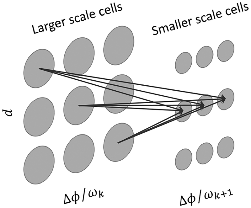
We therefore extended Chen and Qian’s model to resolve the above problems. The first extension is to replace the artificial selection procedure by multiplicative connections from large to small scales. Let the position- and phase-shift parameters of pre- and post-synaptic cells be d_pre, Δϕ_pre, d_post and Δϕ_post respectively. The connection strength is set to:

$$W(d_{\text{post}},d_{\text{pre}},\mathrm{\Delta }{\varphi }_{\text{pre}})=\text{exp}\left(-\frac{{\left[d_{\text{post}}-\left(d_{\text{pre}}+\frac{\mathrm{\Delta }{\varphi }_{\text{pre}}}{{\omega }_{\text{pre}}}\right)\right]}^2}{{\sigma }_d^2}\right)$$ (14)

where ω_pre is the preferred spatial frequency of pre-synaptic cell. Thus, the connection is the strongest when the pre-synaptic cell’s overall preferred disparity (as determined by its both position and phase shifts) equals the post-synaptic cell’s position shift. This is illustrated schematically in Fig. 2. σ_d controls the spread of connections around the strongest connections. We used σ_d = 0.1 pixel in our simulations but other values work well too (see below). Note that the connections are local as Eqn. 14 applies to cells tuned to each location (x, y). For simplicity, the above description uses the pooled responses indexed by d and Δϕ. However, an equivalent description can be made with responses before pooling, which effectively combines the pooling and multiplication steps into one.

Figure 2:

Schematic drawing of the multiplicative connections from cells of a larger scale to cells of the next smaller scale (Eqn. 14). For each scale and image location, the cells are indexed by their position-shift and phase-shift parameters. To avoid clutter, only the strongest connections from three pre-synaptic cells to three post-synaptic cells are shown. The three pre-synaptic cells lie on a negative diagonal line and thus have the same total preferred disparity (Eqn. 10). The three post-synaptic cells have the same position shift equal to the pre-synaptic cells’ total preferred disparity. Each cell’s RFs also receive inputs from stimuli (not shown) to compute energy responses.

The final response of a cell is a multiplication of its energy response to the stimulus and the total gain it receives from the previous scale. Similar to the iteration in Chen and Qian (2004), the response is locally determined. For each position (x, y), denote the energy response after spatial and orientation pooling as r(σ, d, Δϕ; x, y) as in Eqn. 11, and the activity of each cell after the gain multiplication as $\tilde{r}(\sigma ,d,\mathrm{\Delta }\varphi ;x,y)$. $\tilde{r}$, then:

$$\begin{gathered} \tilde{r}(\sigma ,d_{\text{post}},\mathrm{\Delta }{\varphi }_{\text{post}};x,y)\equiv r(\sigma ,d_{\text{post}},\mathrm{\Delta }{\varphi }_{\text{post}};x,y) \\ \cdot \sum _{d_{\text{pre}},\mathrm{\Delta }{\varphi }_{\text{pre}}}W(d_{\text{post}},d_{\text{pre}},\mathrm{\Delta }{\varphi }_{\text{pre}})\tilde{r}(\beta \sigma ,d_{\text{pre}},\mathrm{\Delta }{\varphi }_{\text{pre}};x,y) \end{gathered}$$ (15)

where β is a constant specifying the ratio of two adjacent scales. As in Chen and Qian, we let $\beta =\sqrt{2}$, and used 5 scales with σ equal to 8, 5.7,4, 2.8 and 2 pixels, respectively. For the largest scale $\tilde{r}(\sigma ,d,\mathrm{\Delta }\varphi ;x,y)\equiv r_{\text{c}}(\sigma ,d,\mathrm{\Delta }\varphi ;x,y)$.

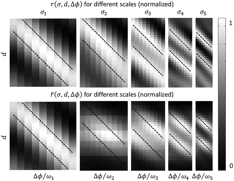
This pattern of connectivity encourages the next scale to use the position-shift RF component to offset the disparities estimated in the previous scale, and to use the phase-shift RF component to estimate residual disparities (i.e., the differences between the actual disparities and their current estimates). It thus provides a physiologically plausible implementation of the coarse-to-fine computation in Chen and Qian (2004). Fig. 3 shows an example of population responses without (top row) and with (bottom row) multiplicative gains for a fixed position in the transparent random-dot stereogram of Fig. 1. The two left-most panels (for the largest scale) are identical. However, at the finest scale, the responses with and without the coarse-to-fine connections are different. Specifically, the connections help reduce false peaks and enhance the correct peaks in the population responses. Moreover, the responses peaks are more focused around Δϕ = 0 as intended in Chen and Qian (2004)’s coarse-to-fine model.

Figure 3:

The energy responses (top row) and the responses multiplied by the coarse-to-fine gains (bottom row) at a fixed position in the transparent random-dot stereogram of Fig. 1. Different columns show results from different scales. In each panel, the horizontal axis represents the cells’ phase-shift parameter Δϕ (divided by ω to covert to disparity), and the vertical axis represents their position-shift parameter d. Dotted lines indicate combinations of phase and position shifts that equal the true disparities of the stimulus.

2.3. Decoding multiple disparities from population responses

Our second extension is to replace the single-disparity decoding in Chen and Qian by multi-disparity decoding. For each scale and location, the decoding finds all reliable peaks in the population responses of cells with various position- and phase-shift parameters. Denote the population response at scale σ and position (x, y) as $\tilde{r}(d,\mathrm{\Delta }\varphi ;\sigma ,x,y)$. Since the coarse-to-fine computation aims to use RF position shifts to offset stimulus disparities computed by the RF phase shifts so that at the end the most responsive cells have Δϕ near 0 Chen and Qian (2004), the decoding method should find all $\widehat{D}\text{s}$ that satisfy:

$${\frac{\partial \tilde{r}(d,\mathrm{\Delta }\varphi ;\sigma ,x,y)}{\partial d}|}_{d=\widehat{D},\mathrm{\Delta }\varphi =0}=0$$ (16)

$${\frac{\partial \tilde{r}(d,\mathrm{\Delta }\varphi ;\sigma ,x,y)}{\partial \mathrm{\Delta }d}|}_{d=\widehat{D},\mathrm{\Delta }\varphi =0}=0$$ (17)

To eliminate noisy small peaks, we require:

$$\tilde{r}(\widehat{D},0)>\alpha \underset{d}{\text{max}}\tilde{r}(d,0)$$ (18)

where 0 < α < 1 is a relative threshold for the peaks as fraction of the highest peak. We let α = 0.3 but its exact value is not important (see below). In our implementation, we used parabolic interpolation to determine $\widehat{D}$. More details are described in Appendix.

We also tried another decoding method by first integrating responses of the cells with the same preferred disparity D* (cf., Eqn. 10):

$${\tilde{r}}_{\text{sum}}(D^{*})={\int }_{-\pi }^{\pi }\text{d}\mathrm{\Delta }\varphi \tilde{r}(D^{*}-\frac{\mathrm{\Delta }\varphi }{\omega },\mathrm{\Delta }\varphi )$$ (19)

and then finding local maxima of ${\tilde{r}}_{\text{sum}}$ as the decoded disparity $\widehat{D}$. We applied 2D interpolation in the d-Δϕ space to perform the integration. A relative threshold α as in Eqn. 18 is also used to remove small noisy peaks.

Although this method integrates responses to reduce noise, it performs slightly worse than the first method. This is likely because the first method takes advantage of the fact that the energy units encode disparity most accurately when the RF position shifts correctly offset the stimulus disparities and thus the phase shifts of the most responsive cell are around Δϕ = 0 (Chen and Qian, 2004).

3. Results

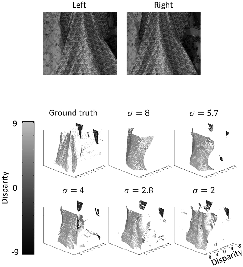
We applied our extended model to a variety of stereograms using exactly the same set of parameters. Since the ground truth of the natural-image stereogram in Fig. 9 represent near and far disparities as positive and negative, respectively, we use the same convention for all stereograms for consistency.

Figure 9:

Model performance on a natural-image stereogram. The top row shows the image pair of “Cloth4” stereogram from Middlebury Stereo Datasets (Hirschmuller and Scharstein, 2007; Scharstein and Pal, 2007). The ground truth and the model performance are shown below. The original image pairs were shifted by 125 pixels and down-sampled by a factor of 10 so that the disparities are within the range covered by the model cells.

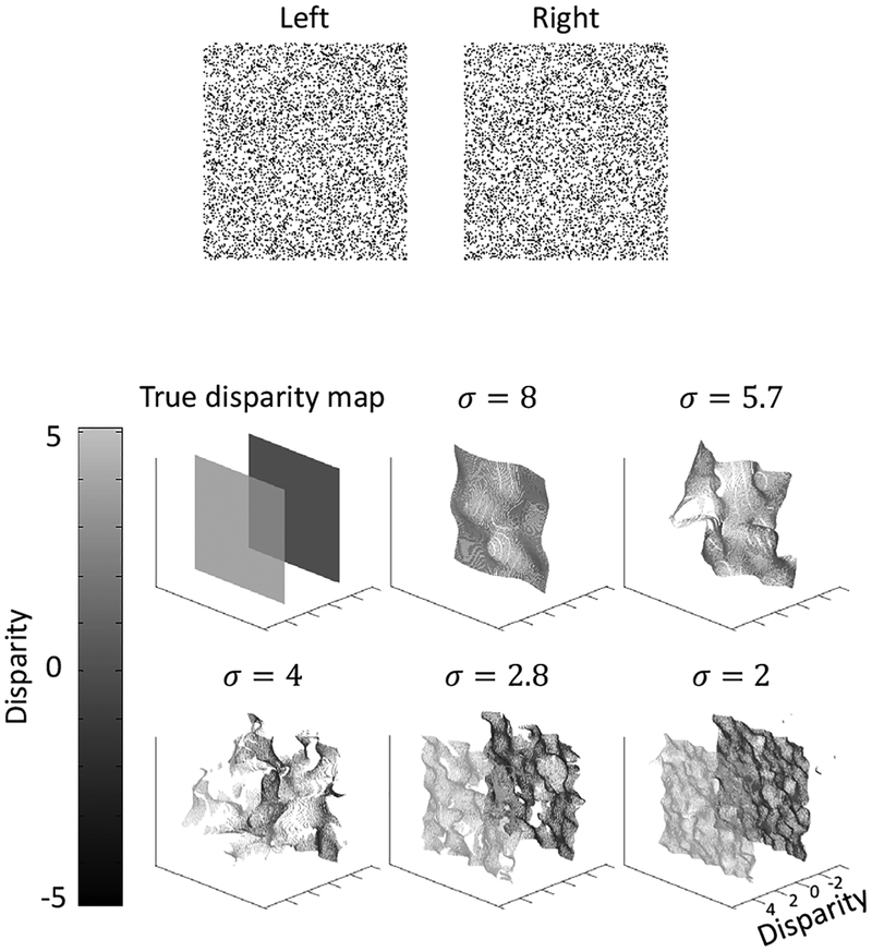
3.1. A transparent stereogram with two overlapping fronto-parallel planes

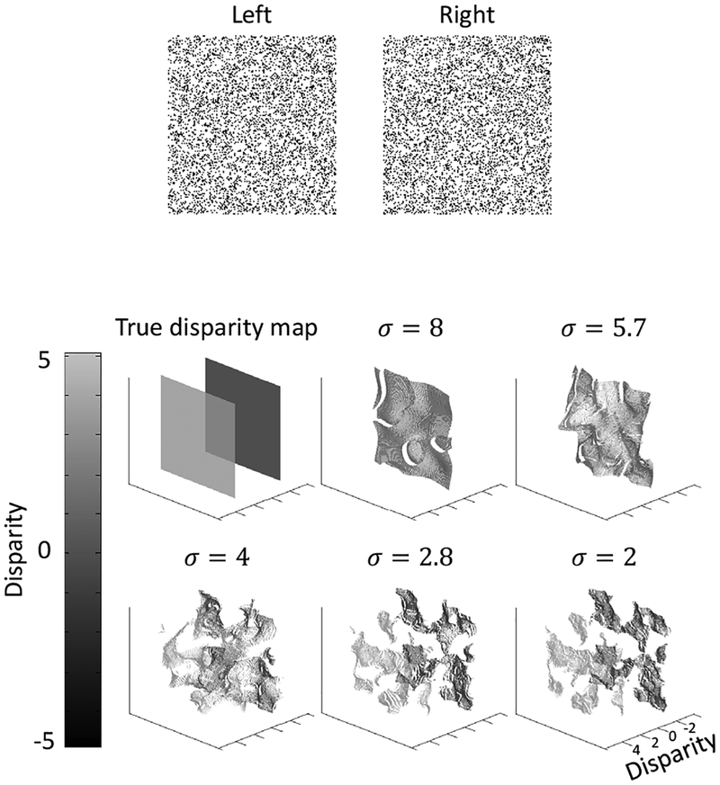
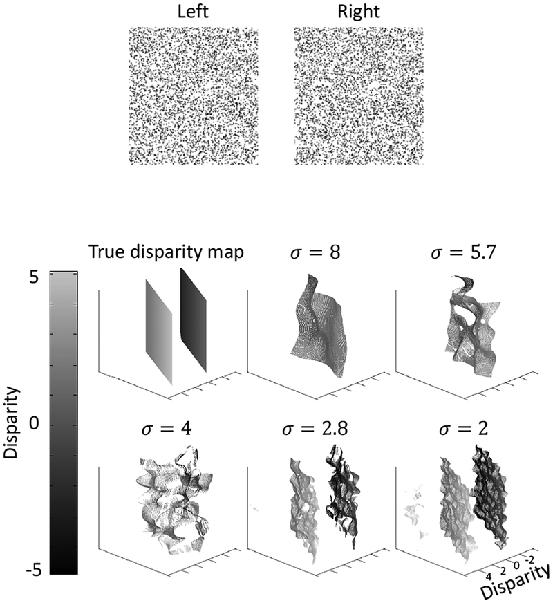
We first applied the model to the same transparent random-dot stereogram as in Fig. 1 (copied to top panel of Fig. 4). The true disparity map and the decoded disparity maps at each scale are shown in the bottom of Fig. 4.

Figure 4:

Model performance on the same transparent random-dot stereogram as in Fig. 1 with two overlapping fronto-parallel planes. The stereogram is shown in the top. The true disparity map and computed maps at the five scales are shown in the bottom.

98.3% of all image positions has two decoded disparities, whereas 1.5% positions has one decoded disparity and 0.2% position has more than two decoded disparities. Thus, the model correctly represented the two transparent planes in most positions. The decoded disparity values are also close to the true values: the root mean square (RMS) error is 0.2 pixel, compared with the 5-pixel separation between the two planes.

The small fluctuations of the decoded disparity values are likely attributable to the fact that our model is completely local, with separate estimation of disparities at each location. Interactions among different positions in higher-level surface representations would likely smooth out the fluctuations.

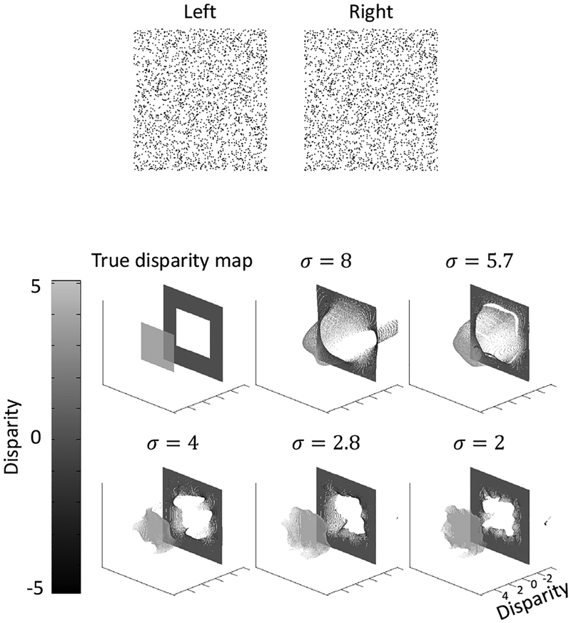
3.2. A non-transparent stereogram with a floating square

To ensure that our model works on non-transparent stereograms, we applied it to a standard random dot stereogram with a floating square. The result is shown in Fig. 5. At the finest scale, our model correctly decoded the floating square.

Figure 5:

Model performance on a standard non-transparent stereogram with a floating square.

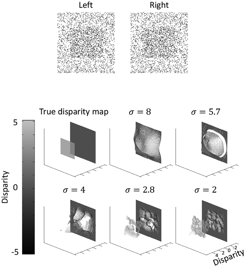
3.3. A transparent stereogram with a floating square

Next, we tested a transparent version of the standard stereogram in the previous example, namely that we added an overlapping background for the central floating square. This is an interesting test because unlike the uniform transparent stereogram in Fig. 4, this stereogram has depth boundaries in addition to transparency. Additionally, the dot density in the central square region is twice as that in the surround region. Nevertheless, the model with the fixed set of parameters work well. The results are shown in Fig. 6.

Figure 6:

Model performance on a transparent stereogram with a floating square.

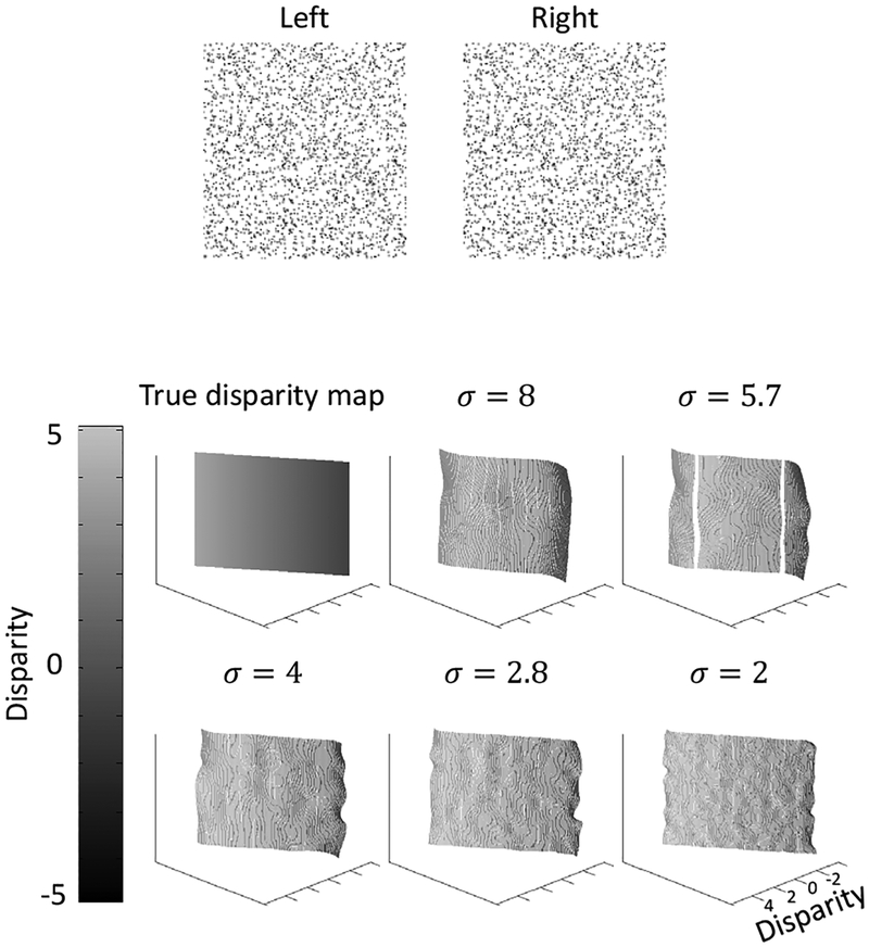
3.4. A non-transparent stereogram with a slanted plane

A problem with Marr and Poggio’s model and related models is that they have difficulty with slanted planes because they consider a small number of fronto-parallel planes and include strong interactions within each plane. In contrast, Chen and Qian (2004)’s coarse-to-fine disparity energy model can compute disparity maps from nontransparent stereograms with slated planes. We therefore also tested our extension on a non-transparent stereogram with a slated plane and the result is shown in Fig. 7.

Figure 7:

Model performance on a non-transparent stereogram with a slanted plane.

3.5. A transparent stereogram with overlapping slanted planes

We then tested a transparent version of the previous stereogram, namely a transparent stereogram with two overlapping slanted planes. The result is shown in Fig. 8.

Figure 8:

Model performance on a transparent stereogram with overlapping slanted planes.

3.6. A natural-image stereogram

Finally, since Chen and Qian (2004)’s model has been applied to natural-image stereograms, we also tested our extension on a natural-image stereogram in which disparity and contrast co-vary, and the result is shown in Fig. 9.

3.7. Disparity attraction and repulsion in transparent stereograms

Disparities of a few isolated features appear to attract or repel each other depending on the features’ lateral separations (Westheimer, 1986; Westheimer and Levi, 1987). Mikaelian and Qian (2000) applied the disparity energy model to explain this observation. A similar phenomenon occurs for transparent stereograms: disparities of two overlapping planes appear to attract or repel each other depending on the depth separation between the planes (Parker and Yang, 1989; Stevenson et al., 1989). Specifically, when the depth separation is small, the two planes appear to merge as a single plane with the average disparity. With increasing separation, the stimulus looks like a thickened slab, a perception termed “pyknostereopsis.” Further depth separation produces two transparent planes with an exaggerated depth separation between them. Finally, at even greater depth separations, the perceived separation between the two planes become veridical.

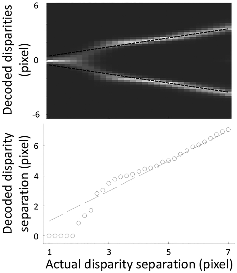
Our model reproduces these observations as shown in Fig. 10. We applied our model to a transparent random-dot stereogram with various disparity separations between two overlapping planes. The disparities of the two planes always have the same magnitude but opposite signs. In the top panel of Fig. 10, each column is a gray-scale histogram (compiled from all positions of the stereogram) of the decoded disparity values for each actual disparity separation between the planes. Brighter colors represent more frequently decoded values. The two actual disparities are indicated by the two dashed black lines. Similar to our perception, the model requires a minimum disparity separation (threshold) between the planes to decode two disparities. This threshold depends on the model’s finest RF scale. Also similar to our perception, the model produces a thickened slab during the transition from decoding one plane to two planes.

Figure 10:

Disparity interactions in stereo transparency. In the top panel, each column shows a decoded-disparity histogram for each actual disparity separation between the two planes in a transparent random-dot stereogram. Brighter colors indicate more frequently decoded values. The two actual disparities are represented by the two black dashed lines. The model explains three observed perceptual regimes with increasing disparity separation, namely depth averaging (one plane), pyknostereopsis (thickening), and transparency (two planes). The bottom panel shows the decoded disparity separation, according to the peaks of the histograms, against the actual disparity separation. The dashed line marks equality between the computed and actual disparity separations. The computed separations show attraction (below the dashed line) and repulsion (above the dashed line) depending on the actual disparity separation.

Averaging two disparities into one may be viewed as an extreme case of attraction between the two disparities. To examine disparity interactions generally, we plot in the bottom panel of Fig. 10 the decoded disparity separation against the actual disparity separation between the two planes (open dots). This was done by searching for the peaks in the histogram of the top panel around the actual disparity values and then subtract the two peak disparities. The dashed line in the bottom panel marks the equality between the computed and estimated disparity separations. The model predicts smaller than actual separations, larger than actual separations, and veridical separations as the actual separation increases, in agreement with the observation of Stevenson et al. (1991).

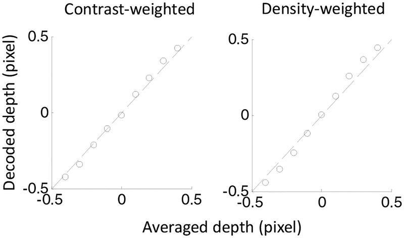
A related observation is that at small disparity separations, the averaged disparity of two overlapping planes is weighted by the contrasts of the dots for the planes Rogers and Anstis (1975). We applied our model to a transparent random-dot stereogram with two planes having ±0.5 pixel of disparities but various contrast ratios between the dots of the two planes. The decoded disparity closely match the average disparity weighted by the contrasts (Fig. 11), in excellent agreement with the observation Rogers and Anstis (1975).

Figure 11:

Disparity averaging weighted by dot contrasts and dot density. We applied our model to a transparent random-dot stereogram with two planes at ±0.5 pixel of disparities, and varied the contrast (left panel) and density (right panel) of the dots of the two planes. Each panel plots the computed disparity against the average disparity weighted by the contrast (left) or density (right).

In addition to contrasts, we also varied the dot density ratio between the two planes. The decoded disparity is very close to the average disparity weighted by the dot densities (Fig. 11, right panel). This is a prediction that could be tested psychophysically.

3.8. Dependence on two key parameters

Our extension introduced two new parameters, and we examined how the model performance depends on them. They are the spread of the connectivity pattern characterized by σ_d in Eqn. 14 and the relative threshold α for eliminating noisy small peaks in decoding in Eqn. 18.

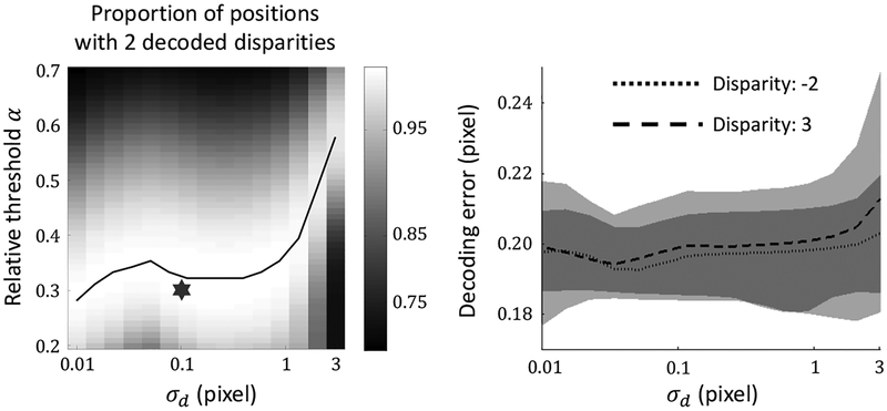
For the transparent stereogram with two fronto-parallel planes in Fig. 4, the right panel of Fig. 12 shows the proportion of positions with two decoded disparities as a function of α and σ_d. The curve in the density plot indicates the optimal combination of the two parameters. When σ_d > 2 pixel, optimal α increases quickly as σ_d increases. This suggests that as the connections for coarse-to-fine computation are more spread out from the intended ones, the ratio of noisy small peaks to real peaks in population responses become larger. For small σ_d, a broad range of α produces similarly good performances. The standard σ_d and α used in our simulations are 0.1 pixel and 0.3 (indicated by a star in the figure.)

Figure 12:

Dependence of the model performance on parameters σ_d and α. We used the same transparent random-dot stereogram as in Fig. 4 with two overlapping planes of disparities −2 and 3 pixels. The left panel shows the proportion of image positions with exactly two decoded disparities as a function of both σ_d and α. Brighter colors indicate higher proportions. The black curve marks the optimal α for each σ_d. The star marks the standard parameters used in all the simulations of this paper. The left panel shows the decoding RMS error as a function of σ_d. α is chosen to be optimal for each σ_d. The two lines are the decoding RMS errors for the two planes. The shaded areas indicate the standard deviations of the errors estimated from 10 different stereograms, and the darker areas indicate overlaps of the shades. The σ_d axis is in log scale for both panels.

The right panel of Fig. 12 shows the decoding RMS error as a function of σ_d (with the optimal α for each σ_d). The model performance does not vary much as long as σ_d is smaller than σ_⊥ of the finest scale (2 pixels in our simulations). These results explain why a single parameter set works well for all stereograms in this paper.

4. Discussion

We extended Chen and Qian’s coarse-to-fine disparity energy model to solve the difficult problem of stereo transparency with biologically plausible mechanisms. In the original model, a given scale decodes a single disparity for each location and uses this disparity to select a set of cells for the next scale. We replaced this artificial selection procedure with multiplicative connections from one scale to the next. The connectivity pattern provides a biologically plausible mechanism to achieve the original model’s goal of using cells’ position-shift RF component to offset stimulus disparities and the more reliable phase-shift RF component to estimate residual disparities. More importantly, whereas each scale of the original model commits to a single decoded disparity at each location, the new model maintains the entire population responses during the coarse-to-fine computation. Consequently, unlike the original model, explicit disparity decoding at each scale is unnecessary for the new model. We can still decode the population responses at each scale for the sole purpose of visualization as we did in this paper. This leads to our second extension: we used a simple threshold criterion capable of decoding multiple disparities, instead of single-disparity decoding in the original model. We demonstrated through computer simulations, with a single parameter set, that these extensions allow our model to solve various transparent and non-transparent stereograms in a biologically plausible way. Finally, our model explains disparity interactions (averaging, thickening, attraction, and repulsion) as the separation between two overlapping planes varies.

Both Chen and Qian (2004)’s model and our current extension use the position-shift RF component to offset estimated stimulus disparities and the phase-shift component to estimate the residual disparities. Consequently, at the end of computation, the most responsive cells have position shifts near stimulus disparities and phase shifts near 0. As we noted above, this strategy is based on the finding that the phase-shift population response is more reliable than the position-shift population response for disparity computation (Chen and Qian, 2004; Tsang and Shi, 2004). The analysis in Appendix shows that this remains true when stimulus disparity is divided evenly between the two eyes. Position shifts are needed to properly place the limited disparity range of phase shifts. Also note that Read and Cumming (2007) follow Chen and Qian (2004) in searching for the cells whose position shift offsets stimulus disparity and whose phase shift is near 0, albeit with a different algorithm.

It is easy to understand why position-shift RFs are generally less reliable than the phase-shift RFs. Consider disparity encoding at a given location by a set of energy units with a range of preferred disparities. If the units have phase-shift RFs, then the RFs of all the units cover the same left and right image patches. Consequently, variations in the units’ responses are attributable to their different tuning properties. In contrast, if the units have position-shift RFs, then different units cover different left and right image patches, which introduce additional variability in the population responses.

We mentioned in Introduction that cells with small RFs can reliably compute only small disparities. This is easy to understand for phase-shift RFs because phase shift is periodic, and disparity representation is unambiguous only for phase shifts within the [−π,π) range (Qian, 1994). One might argue that because position shift is not periodic, position-shift RFs could represent arbitrarily large disparities. However, this is not the case for the reason discussed in the above paragraph. Specifically, by definition, cells with different position shifts are located at different positions. When their RFs are small, they more likely cover completely different image regions. Thus, spatial variations of image properties (contrast, frequency content, local features such as orientation, etc.) may overwhelm the disparity related signals in population responses.

How does our extended coarse-to-fine disparity energy model solve the stereo transparency problem? We define residual disparity as the difference between an actual stimulus disparity and its current estimate. At the largest scale, cells’ RFs cover many dots carrying different disparities and thus the most responsive cells are likely those tuned to the average of the stimulus disparities (see Fig. 3 and 4). Because of the connectivity pattern, these cells will excite the cells in the next scale whose position-shift components are close to the average disparity. With the offsetting of the average disparity by the position shifts, the cells of the next scale with smaller RFs can better represent the residual disparities with their phase shifts. This process is then repeated to gradually offset more of the stimulus disparities and reduce the residual disparities. At the smallest scale, the most active cells are the ones whose position shifts are close to one of the actual stimulus disparities and whose phase-shift components are near 0 (because the residual disparities are close to 0).

Our model makes specific predictions. There are physiological and psychophysical evidence for coarse-to-fine disparity processing in biological vision (Menz and Freeman, 2003; Smallman and MacLeod, 1994; Wilson et al., 1991; Rohaly and Wilson, 1993). Our model suggests a specific implementation of this computation, namely that the connections from cells with larger RFs to those with smaller RFs is the strongest when a pre-synaptic cell’s overall preferred disparity (as determined by its both position and phase shifts) matches the post-synaptic cell’s position shift. A second prediction is that the smallest disparity separation between two transparent surfaces that can be resolved perceptually is determined by the RF sizes of the finest scale in the coarse-to-fine process. This could be tested by examining whether the smallest resolvable disparity separation increases with retinal eccentricity. Our model also predicts that disparity averaging should be weighted by dot densities (Fig. 11).

In conclusion, we have extended Chen and Qian (2004)’s coarse-to-fine disparity energy model to solve the difficult problem of stereo transparency with biologically plausible mechanisms. The model uses both position-shift and phase-shift RF components and works well on a variety of transparent and non-transparent stereograms. Although large-scale cells tend to average stimulus disparities and small-scale cells cannot compute large stimulus disparities, combining information through the coase-to-fine process solves the transparency problem. Our model also makes specific predictions on connectivity between disparity tuned cells of different scales and on our perception of stereo transparency.

Appendix

Quadrature pair responses and preferred disparities

The derivations here are similar to our previous derivations (Chen and Qian, 2004) but with stimulus disparities evenly divided between the two eyes’ oriented RFs with both position and phase shifts.

The RFs of simple cells in a quadrature pair are defined in Eqn. 2, 3, 4, and 5 of the text. For a stimulus I (x, y) with disparity D, the images for the two eyes are

$$I_{\text{L}}(x,y)=I(x-\frac{D}{2},y)$$ (20)

$$I_{\text{R}}(x,y)=I(x+\frac{D}{2},y)$$ (21)

Without loss of generality, for position (0, 0) Eqn. 6 and 7 become

$$\begin{gathered} r_1(0,0)=\int \text{d}x\text{d}yI(x-\frac{D}{2},y)\frac{1}{2\pi {\sigma }_{\perp }{\sigma }_{\parallel }}{e}^{-\frac{x_1^2}{2{\sigma }_{\perp }^2}-\frac{y_1^2}{2{\sigma }_{\parallel }^2}}\text{cos}\left(\omega x_1-\frac{\mathrm{\Delta }\varphi }{2}\right) \\ +\int \text{d}x\text{d}yI(x+\frac{D}{2},y)\frac{1}{2\pi {\sigma }_{\perp }{\sigma }_{\parallel }}{e}^{-\frac{x_2^2}{2{\sigma }_{\perp }^2}-\frac{y_2^2}{2{\sigma }_{\parallel }^2}}\text{cos}\left(\omega x_2+\frac{\mathrm{\Delta }\varphi }{2}\right) \end{gathered}$$ (22)

$$\begin{gathered} r_2(0,0)=\int \text{d}x\text{d}yI(x-\frac{D}{2},y)\frac{1}{2\pi {\sigma }_{\perp }{\sigma }_{\parallel }}{e}^{-\frac{x_1^2}{2{\sigma }_{\perp }^2}-\frac{y_1^2}{2{\sigma }_{\parallel }^2}}\text{sin}\left(\omega x_1-\frac{\mathrm{\Delta }\varphi }{2}\right) \\ +\int \text{d}x\text{d}yI(x+\frac{D}{2},y)\frac{1}{2\pi {\sigma }_{\perp }{\sigma }_{\parallel }}{e}^{-\frac{x_2^2}{2{\sigma }_{\perp }^2}-\frac{y_2^2}{2{\sigma }_{\parallel }^2}}\text{sin}\left(\omega x_2+\frac{\mathrm{\Delta }\varphi }{2}\right) \end{gathered}$$ (23)

in which x₁, y₁, x₂, y₂ are rotated coordinates defined as

$$\left(\begin{array}{c}{x}_1\\ y_1\end{array}\right)=\left(\begin{array}{cc}\text{sin}\theta & \text{cos}\theta \\ -\text{cos}\theta & \text{sin}\theta \end{array}\right)\left(\begin{array}{c}x-\frac{d}{2}\\ y\end{array}\right)$$ (24)

$$\left(\begin{array}{c}{x}_2\\ y_2\end{array}\right)=\left(\begin{array}{cc}\text{sin}\theta & \text{cos}\theta \\ -\text{cos}\theta & \text{sin}\theta \end{array}\right)\left(\begin{array}{c}x+\frac{d}{2}\\ y\end{array}\right)$$ (25)

Therefore, the quadrature-pair response is

$$\begin{gathered} r_{\text{c}}=\frac{1}{2\pi {\sigma }_{\perp }{\sigma }_{\parallel }}|\int \text{d}x\text{d}yI(x-\frac{D}{2},y)e^{-\frac{x_1^2}{2{\sigma }_{\perp }^2}-\frac{y_1^2}{2{\sigma }_{\parallel }^2}}{e}^{i(\omega x_1-\frac{\mathrm{\Delta }\varphi }{2})} \\ +{\int \text{d}x\text{d}yI(x+\frac{D}{2},y)e^{-\frac{x_2^2}{2{\sigma }_{\perp }^2}-\frac{y_2^2}{2{\sigma }_{\parallel }^2}}{e}^{i(\omega x_2+\frac{\mathrm{\Delta }\varphi }{2})}|}^2 \\ =\frac{1}{2\pi {\sigma }_{\perp }{\sigma }_{\parallel }}|e^{i\frac{\omega \text{sin}\theta (D-d)-\mathrm{\Delta }\varphi }{2}}{\int \text{d}x\text{d}yI(x,y)e}^{-\frac{{x^{\prime }}_1^2}{2{\sigma }_{\perp }^2}-\frac{{y^{\prime }}_1^2}{2{\sigma }_{\parallel }^2}}{e}^{i\omega (\text{sin}\theta x+\text{cos}\theta y)} \\ +{e^{i\frac{\omega \text{sin}\theta (-D+d)+\mathrm{\Delta }\varphi }{2}}{\int \text{d}x\text{d}yI(x,y)e}^{-\frac{{x^{\prime }}_2^2}{2{\sigma }_{\perp }^2}-\frac{{y^{\prime }}_2^2}{2{\sigma }_{\parallel }^2}}{e}^{i\omega (\text{sin}\theta x+\text{cos}\theta y)}|}^2 \end{gathered}$$ (26)

with

$$\left(\begin{array}{c}{x^{\prime }}_1\\ {y^{\prime }}_1\end{array}\right)=\left(\begin{array}{cc}\text{sin}\theta & \text{cos}\theta \\ -\text{cos}\theta & \text{sin}\theta \end{array}\right)\left(\begin{array}{c}x-\frac{d-D}{2}\\ y\end{array}\right)$$ (27)

$$\left(\begin{array}{c}{x^{\prime }}_2\\ {y^{\prime }}_2\end{array}\right)=\left(\begin{array}{cc}\text{sin}\theta & \text{cos}\theta \\ -\text{cos}\theta & \text{sin}\theta \end{array}\right)\left(\begin{array}{c}x+\frac{d-D}{2}\\ y\end{array}\right)$$ (28)

The first order approximation of exp $\left[-\frac{{(x+\mathrm{\Delta }x)}^2}{2{\sigma }^2}\right]$ with respect to Δx is

$$\text{exp}\left[-\frac{{\left(x+\mathrm{\Delta }x\right)}^2}{2{\sigma }^2}\right]\approx \text{exp}\left(-\frac{x^2}{2{\sigma }^2}\right)\left(1-\frac{x\mathrm{\Delta }x}{{\sigma }^2}\right)$$ (29)

Define a Gaussian envelope as

$$G_{\text{Gauss}}(x,y)=\frac{1}{2\pi {\sigma }_{\perp }{\sigma }_{\parallel }}\text{exp}\left(-\frac{{(\text{sin}\theta x+\text{cos}\theta y)}^2}{2{\sigma }_{\perp }^2}-\frac{{(-\text{cos}\theta x+\text{sin}\theta y)}^2}{2{\sigma }_{\parallel }^2}\right)$$ (30)

and define the original image filtered by this Gaussian envelope and its scaled first partial derivative with respect to x as

$$I_1(x,y)=G_{\text{Gauss}}(x,y)I(x,y)$$ (31)

$$\begin{gathered} I_2(x,y)={\sigma }_{\perp }\frac{\partial G_{\text{Gauss}}(x,y)}{\partial x}I(x,y) \\ =\left(-\frac{\text{sin}\theta (\text{sin}\theta x+\text{cos}\theta y)}{{\sigma }_{\perp }}-\frac{-\text{cos}\theta (-\text{cos}\theta x+\text{sin}\theta y)}{k^2{\sigma }_{\perp }}\right)I_1(x,y) \end{gathered}$$ (32)

where $k=\frac{{\sigma }_{\parallel }}{{\sigma }_{\perp }}$ is the RF aspect ratio. The Fourier component at frequency (ω sin θ, ω cos θ) of I₁ and I₂ are

$$A=\int \text{d}x\text{d}y{e}^{i(\omega \text{sin}\theta x+\omega \text{cos}\theta y)}{I}_1(x,y)$$ (33)

$$B=\int \text{d}x\text{d}y{e}^{i(\omega \text{sin}\theta x+\omega \text{cos}\theta y)}{I}_2(x,y)$$ (34)

With these notations, along with $\delta =\frac{\omega \text{sin}\theta (D-d)-\mathrm{\Delta }\varphi }{2}$, the complex cell response is

$$\begin{gathered} r_{\text{c}}\approx {\left|e^{\text{i}\delta }\left(A-\frac{d-D}{2{\sigma }_{\perp }}B\right)+e^{-\text{i}\delta }\left(A+\frac{d-D}{2{\sigma }_{\perp }}B\right)\right|}^2 \\ ={\left|2A\text{cos}\delta +i\frac{D-d}{{\sigma }_{\perp }}B\text{sin}\delta \right|}^2 \\ \approx 4{\left|A\right|}^2{\text{cos}}^2\delta +{\left(\frac{D-d}{{\sigma }_{\perp }}\right)}^2{\left|B\right|}^2{\text{sin}}^2\delta \end{gathered}$$ (35)

which is an approximation to the second order of $\frac{D-d}{{\sigma }_{\perp }}$. If the stimulus disparity D is largely offset by cells’ position shift d, then the second term is small, and the cells’ preferred disparity is determined by the first term, resulting in Eqn. 10 in the text.

Eqn. 35 also demonstrates that phase-shift population responses (from cells with a fixed d but a full range of Δϕ) are more reliable than position-shift population responses (from cells with a fixed Δϕ but a range of d) even when disparity is evenly divided between the two eyes. Specifically, the second term of Eqn. 35 can be made small when D is largely offset by a fixed d, and the cells with this d and the full range of Δϕ have a reliable peak determined by the first term. In contrast, the second term cannot always be small for a fixed Δϕ and a range of d, contaminating the first term. Also note that when Δϕ = 0, the position-shift population response is symmetric around d − D (Read and Cumming, 2007). However, this symmetry only holds for the special case of uniform disparity.

Disparity decoding in discrete form

We explain the detailed implementation of disparity decoding. As mentioned in Sec. 2.3, we aim to find $\widehat{D}$ satisfying Eqn. 16, 17 and 18. We can only approximately achieve this goal since the population responses are sampled from cells with a discrete set of parameters d and Δϕ.

For a given scale (σ) and spatial location (x and y), local population responses $\tilde{r}(d_i,\mathrm{\Delta }{\varphi }_j)$ are stored in a 2-D array,

$${\tilde{r}}_{i,j}=\tilde{r}(d_i,\mathrm{\Delta }{\varphi }_j)$$

in which d_i and Δϕ_j indicate the position- and phase-shift parameters of the cells. For convenience, we use j₀ to index the cell whose Δϕ_j0 = 0.

The algorithm first finds all i’s satisfying

$${\tilde{r}}_{i,j_0}>{\tilde{r}}_{i-1,j_0},{\tilde{r}}_{i,j_0}>{\tilde{r}}_{i+1,j_0}\text{and}{\tilde{r}}_{i,j_0}>\alpha \underset{i}{\text{max}}{\tilde{r}}_{i,j_0}$$

Then, for each d_i so determined, it is reasonable to assume that $\widehat{D}$ falls within [d_{i− 1}, d_i+1]. Define Δd ≡ d_i − d_i−1 = d_i+1 − d_i. We search for j over $\frac{\mathrm{\Delta }{\varphi }_j}{\omega }\in [-\mathrm{\Delta }d,\mathrm{\Delta }d]$ according to ${\tilde{r}}_{i,j}>{\tilde{r}}_{i,j-1}$ and ${\tilde{r}}_{i,j}>{\tilde{r}}_{i,j+1}$. Apply parabolic interpolation on ${\tilde{r}}_{i,j-1}$, ${\tilde{r}}_{i,j}$ and ${\tilde{r}}_{i,j+1}$, we find the peak position of Δϕ*, and let:

$$\widehat{D}=d_i+\frac{\mathrm{\Delta }{\varphi }^{*}}{\omega }$$

References

- Anzai A, Ohzawa I, and Freeman RD (1997). Neural mechanisms underlying binocular fusion and stereopsis: Position vs.phase. Proceedings of the National Academy of Sciences, 94(10):5438–5443. [DOI] [PMC free article] [PubMed] [Google Scholar]
- Anzai A, Ohzawa I, and Freeman RD (1999). Neural mechanisms for processing binocular information i. simple cells. Journal of Neurophysiology, 82(2):891–908. [DOI] [PubMed] [Google Scholar]
- Assee A and Qian N (2007). Solving da vinci stereopsis with depth-edge-selective v2 cells. Vision Research, 47(20):2585–2602. [DOI] [PMC free article] [PubMed] [Google Scholar]
- Chen Y and Qian N (2004). A coarse-to-fine disparity energy model with both phase-shift and position-shift receptive field mechanisms. Neural Computation, 16(8):1545–1577. [DOI] [PubMed] [Google Scholar]
- Hirschmuller H and Scharstein D (2007). Evaluation of cost functions for stereo matching. In Computer Vision and Pattern Recognition, 2007. CVPR ‘07. IEEE Conference on, pages 1–8. [Google Scholar]
- Julesz B (1971). Foundations of cyclopean perception, volume 4 University of Chicago Press. [Google Scholar]
- Li Z and Qian N (2014). Solving stereo transparency with an extended coarse-to-fine disparity energy model. VSS2014 Talk. [DOI] [PMC free article] [PubMed] [Google Scholar]
- Livingstone MS and Tsao DY (1999). Receptive fields of disparity-selective neurons in macaque striate cortex. Nat Neurosci, 2(9):825–832. 10.1038/12199. [DOI] [PubMed] [Google Scholar]
- Mansfield JS and Parker AJ (1993). An orientation-tuned component in the contrast masking of stereopsis. Vision Research, 33(11):1535–1544. [DOI] [PubMed] [Google Scholar]
- Marr D and Poggio T (1976). Cooperative computation of stereo disparity. Science, 194(4262):283–287. [DOI] [PubMed] [Google Scholar]
- Marr D and Poggio T (1979). A computational theory of human stereo vision. Proceedings of the Royal Society of London. Series B. Biological Sciences, 204(1156):301–328. [DOI] [PubMed] [Google Scholar]
- Menz MD and Freeman RD (2003). Stereoscopic depth processing in the visual cortex: a coarse-to-fine mechanism. Nat Neurosci, 6(1):59–65. 10.1038/nn986. [DOI] [PubMed] [Google Scholar]
- Mikaelian S and Qian N (2000). A physiologically-based explanation of disparity attraction and repulsion. Vision Research, 40(21):2999–3016. [DOI] [PubMed] [Google Scholar]
- Ohzawa I, DeAngelis GC, and Freeman RD (1990). Stereoscopic depth discrimination in the visual cortex: neurons ideally suited as disparity detectors. Science, 249(4972):1037–1041. [DOI] [PubMed] [Google Scholar]
- Ohzawa I, DeAngelis GC, and Freeman RD (1997). Encoding of binocular disparity by complex cells in the cat’s visual cortex. Journal of Neurophysiology, 77(6):2879–2909. [DOI] [PubMed] [Google Scholar]
- Parker AJ and Yang Y (1989). Spatial properties of disparity pooling in human stereo vision. Vision Research, 29(11):1525–1538. [DOI] [PubMed] [Google Scholar]
- Pollard SB, Mayhew JEW, and Frisby JP (1985). Pmf: A stereo correspondence algorithm using a disparity gradient limit. Perception, 14(4):449–470. [DOI] [PubMed] [Google Scholar]
- Prazdny K (1985). Detection of binocular disparities. Biological Cybernetics, 52(2):93–99. [DOI] [PubMed] [Google Scholar]
- Prince S, Cumming BG, and Parker AJ (2002). Range and mechanism of encoding of horizontal disparity in macaque v1. Journal of Neurophysiology, 87(1):209–221. [DOI] [PubMed] [Google Scholar]
- Qian N (1994). Computing stereo disparity and motion with known binocular cell properties. Neural Computation, 6(3):390–404. [Google Scholar]
- Qian N (1997). Binocular disparity and the perception of depth. Neuron, 18(3):359368. [DOI] [PubMed] [Google Scholar]
- Qian N and Sejnowski TJ (1989). Learning to solve random-dot stereograms of dense and transparent surfaces with recurrent backpropagation In Proceedings of the 1988 Connectionist models summer school, pages 435–443. Morgan Kaufmann. [Google Scholar]
- Read JCA and Cumming BG (2007). Sensors for impossible stimuli may solve the stereo correspondence problem. Nat Neurosci, 10(10):1322–1328. 10.1038/nn1951. [DOI] [PMC free article] [PubMed] [Google Scholar]
- Rogers BJ and Anstis SM (1975). Reversed depth from positive and negative stereograms. Perception, 4(2):193–201. [Google Scholar]
- Rohaly AM and Wilson HR (1993). Nature of coarse-to-fine constraints on binocular fusion. Journal of the Optical Society of America A, 10(12):2433–2441. [DOI] [PubMed] [Google Scholar]
- Scharstein D and Pal C (2007). Learning conditional random fields for stereo. In Computer Vision and Pattern Recognition, 2007. CVPR ‘07. IEEE Conference on, pages 1–8. [Google Scholar]
- Schor CM and Wood I (1983). Disparity range for local stereopsis as a function of luminance spatial frequency. Vision Research, 23(12):1649–1654. [DOI] [PubMed] [Google Scholar]
- Smallman HS and MacLeod DIA (1994). Size-disparity correlation in stereopsis at contrast threshold. Journal of the Optical Society of America A, 11(8):2169–2183. [DOI] [PubMed] [Google Scholar]
- Stevenson SB, Cormack LK, and Schor CM (1989). Hyperacuity, superresolution and gap resolution in human stereopsis. Vision Research, 29(11):1597–1605. [DOI] [PubMed] [Google Scholar]
- Stevenson SB, Cormack LK, and Schor CM (1991). Depth attraction and repulsion in random dot stereograms. Vision Research, 31(5):805–813. [DOI] [PubMed] [Google Scholar]
- Tsang EKC and Shi BE (2004). A preference for phase-based disparity in a neuromorphic implementation of the binocular energy model. Neural Computation, 16(8):1579–1600. [DOI] [PubMed] [Google Scholar]
- Westheimer G (1986). Spatial interaction in the domain of disparity signals in human stereoscopic vision. The Journal of Physiology, 370(1):619–629. [DOI] [PMC free article] [PubMed] [Google Scholar]
- Westheimer G and Levi DM (1987). Depth attraction and repulsion of disparate foveal stimuli. Vision Research, 27(8):1361–1368. [DOI] [PubMed] [Google Scholar]
- Wilson HR, Blake R, and Halpern DL (1991). Coarse spatial scales constrain the range of binocular fusion on fine scales. Journal of the Optical Society of America A, 8(1):229–236. [DOI] [PubMed] [Google Scholar]
- Zhaoping L (2002). Preattentive segmentation and correspondence in stereo. Philosophical Transactions of the Royal Society of London. Series B: Biological Sciences, 357(1428):1877–1883. [DOI] [PMC free article] [PubMed] [Google Scholar]
- Zhu Y-D and Qian N (1996). Binocular receptive field models, disparity tuning, and characteristic disparity. Neural Computation, 8(8):1611–1641. [DOI] [PubMed] [Google Scholar]