Controlling an organic synthesis robot with machine learning to search for new reactivity

Abstract

The discovery of chemical reactions is an inherently unpredictable and time-consuming process¹. An attractive alternative is to predict reactivity, although relevant approaches, such as computer-aided reaction design, are still in their infancy. Reaction prediction based on high-level quantum chemical methods is complex, even for simple molecules. Although machine learning is powerful for data analysis, its applications in chemistry are still being developed⁶. Inspired by strategies based on chemists’ intuition, we propose that a reaction system controlled by a machine learning algorithm may be able to explore the space of chemical reactions quickly, especially if trained by an expert. Here we present an organic synthesis robot that can perform chemical reactions and analysis faster than they can be performed manually, as well as predict the reactivity of possible reagent combinations after conducting a small number of experiments, thus effectively navigating chemical reaction space. By using machine learning for decision making, enabled by binary encoding of the chemical inputs, the reactions can be assessed in real time using nuclear magnetic resonance and infrared spectroscopy. The machine learning system was able to predict the reactivity of about 1,000 reaction combinations with accuracy greater than 80 per cent after considering the outcomes of slightly over 10 per cent of the dataset. This approach was also used to calculate the reactivity of published datasets. Further, by using real-time data from our robot, these predictions were followed up manually by a chemist, leading to the discovery of four reactions.

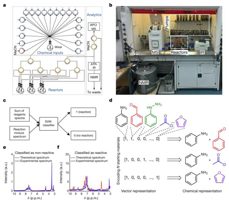
Recent progress in automated chemistry, online analytics and real-time optimization suggests that it is possible to construct a robot that can autonomously explore chemical reactivity. With this in mind, we have designed, built and programmed a bespoke chemical-handling robot comprising in-line spectroscopy, real-time data analysis and feedback mechanisms (Fig. 1a, b). The robot is configured to execute six experiments in parallel, allowing up to 36 experiments to be performed per day. To evaluate the outcome of a reaction, the robot is equipped with real-time sensors—a flow benchtop nuclear magnetic resonance (NMR) system, a mass spectrometer and an attenuated total-reflection infrared spectroscopy system—to record the spectra of the reaction mixtures. Then, it uses an algorithm to automatically classify the reaction mixtures as reactive or non-reactive, which is reported in binary form as zero or one, using a supported vector machine (SVM) with a linear kernel (Fig. 1c) model. This algorithm compares the spectrum of the starting materials with that recorded by the robotic platform using NMR and infrared spectroscopy, registering differences as reactivity hits (see Fig. 1e for an example of a non-reactive mixture and Fig. 1f for a reactive mixture). By training the model on 72 reactive and non-reactive mixtures manually classified by an expert chemist, the model could classify the reactivity of reaction mixtures with an accuracy of 86%, as determined by leave-one-out cross-validation. The machine learning algorithm used to explore the chemical space needs an automatically generated representation of the reactions. Because the representation of the data is crucial for machine learning, we created a reaction descriptor with a width corresponding to the number of starting materials in the pool of reagents and with bits representing reagents that were present in a given reaction mixture to one, similarly to one-hot encoding. Figure 1d shows example vector representations for the model substrate pool consisting aniline, benzaldehyde, acetyl chloride, phenylhydrazine and furan.

Fig. 1. Automatic reaction detection with machine learning.

a, Schematic of the chemical robot. The circles are pumps and the coloured dots are the positions of the valves. APCI, atmospheric pressure chemical ionization; MS, mass spectrometer; ATR-IR, attenuated total reflectance infrared spectrometer. b, Photograph of the chemical robot, showing the pumps, reactors and real-time analytics, including the NMR, MS and infrared (IR) spectroscopy systems. c, SVM workflow for reaction detection using infrared and NMR spectroscopy, utilizing changes in the spectra. d, Reaction space representation using vectors. e, Example of a ¹H NMR (43 MHz, MeCN) spectrum for a non-reactive reaction mixture. a.u., arbitrary units. f, Example of a reaction mixture ¹H NMR (43 MHz, MeCN) spectrum for which a chemical reaction has been detected.

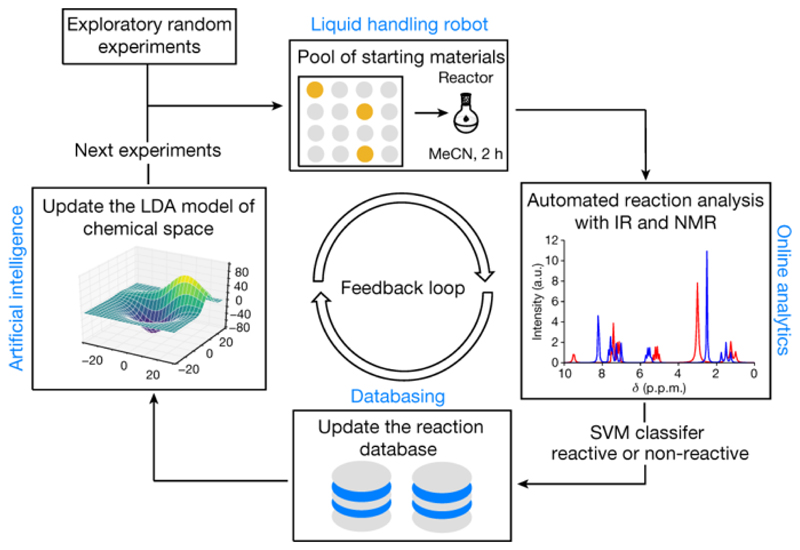
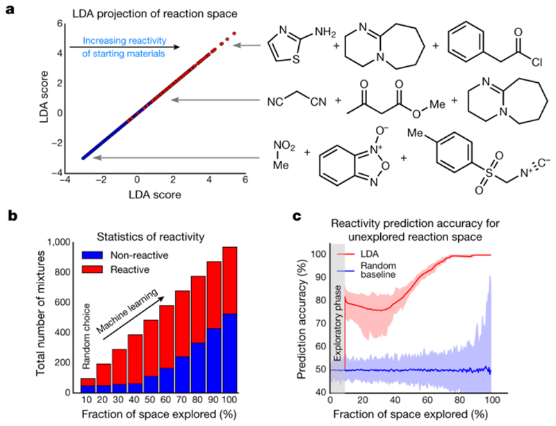
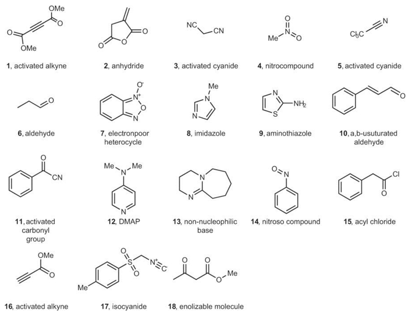
This approach to representing chemical space renders it structure-independent and allows the robotic platform to operate without prior knowledge about reactivity and chemical structure (Fig. 2). Initially, the chemical space was sampled by performing reactions with random combinations of starting materials, evaluating their reactivity as reactive or non-reactive using the SVM model (to determine expected values of reactivity, Y) and encoding them in vector form (to obtain a training set, X). The process of random selection is important because the system avoids making prior assumptions about the possible reactivity of the reagents, ensuring that the initial run results are unknown. Even if the reaction mixture decomposes or is non-reactive, this information is still useful for the navigation of the chemical space, allowing real-time assessment of the reactivity of the starting materials. After the reaction database has been built, a linear discriminant analysis (LDA) model is trained on the data obtained to construct a model of the chemical space. The remaining reactions are then rated by predicting the probability of reactivity using the LDA model. This allows for autonomous decision making, and the reaction with the highest score is performed and analysed by the robotic system, thus avoiding many non-reactive combinations and speeding up the search. The loop is closed by updating the reaction database with the result of the last experiment from the platform and then by retraining the LDA model of the chemical space. The cycle is repeated until the required number of reactions is performed or until the whole space—defined by a pool of 18 reactive, structurally diverse molecules containing functional groups 1–18 (Extended Data Fig. 1)—is spanned. The chemical space constituted of two- and three-component reactions formed from the pool of starting materials, giving 969 possible experiments. When LDA was performed, the algorithm was able to clearly differentiate between reactive and non-reactive combinations of the starting materials (Fig. 3a). This means that the LDA can be useful for predicting new reactivity. By taking this approach, we showed that the robot can learn how reactive the starting materials are and efficiently navigate chemical space. For example, the reaction mixture composed from 2-aminothiazole (9), phenylacetyl chloride (15) and DBU (13) would be classified as highly reactive, a mixture of malononitrile (3), methylacetoacetate (18) and DBU (13) as moderately reactive and a mixture of nitromethane (4), benzofuroxan (7) and toluenesulfonylmethyl isocyanide (17) as non-reactive. These assignments agree with basic chemical intuition, demonstrating the predictive power of the model (see Supplementary Information for the reactivity of all reactions according to the LDA projection).

Fig. 2. Overview of the artificial intelligence algorithm used for the exploration of chemical space with the liquid-handling robot.

The liquid-handling robot performs reactions by choosing reactants from the pool of starting materials. Online analytics is used for real-time interpretation of reaction outcomes as reactive or non-reactive, and the reaction database stores reaction outcomes. Machine learning is used to build a model of the chemical space, recommend the next experiments and control the robot.

Fig. 3. Simulations exploring the chemical space and predictive power of the model.

a, Left, LDA projection of all the reactions performed, demonstrating the predictive power of LDA in classifying the reactivity. Red symbols, reactive combinations; blue symbols, non-reactive combinations. Right, examples of reactions in different regions of chemical space projected by LDA on the basis of collective chemical knowledge acquired by the robot. Top, very reactive; middle, moderately reactive; bottom, non-reactive. b, Simulation showing the number of reactive and non-reactive mixtures chosen by the algorithm during the exploration of chemical space. c, Aggregated results from 100 simulations showing the average accuracy of the LDA in predicting the reactivity versus the fraction of chemical space explored; the confidence intervals are defined by the maximum and minium values.

To further test the learning ability of our robotic system, we performed simulations to calculate the number of reactive versus non-reactive combinations of the starting materials chosen by the algorithm during the exploration of the chemical space (Fig. 3b). In the initial stage, the space was randomly sampled, resulting in an equal number of reactive and non-reactive combinations being chosen by the algorithm. After reaching the desired number of reactions, decisions were made using LDA, leading to a rapid increase in the number of reactive combinations being chosen by the algorithm. In the end, the algorithm identified the empty part of chemical space; that is, the last experiments that were chosen were non-reactive (Fig. 3b). The accuracy of predicting the reactivity is shown in Fig. 3c, which shows that as chemical space is progressively searched, the accuracy of the prediction of the reactivity increases along with the confidence intervals. This demonstrates that the robot can ‘self-learn’ using artificial intelligence by exploiting this reactivity-first approach. Additionally, the accuracy of the LDA classifier in predicting the reactivity of the reaction mixtures was determined as 86% ± 3% using five-fold cross-validation.

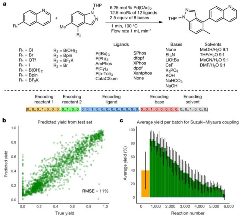
To further explore the predictive power of our approach, we also investigated the Suzuki–Miyaura reaction space (see Fig. 4a) described recently by searching for reactions with the highest yield with our machine learning approach. To achieve this, we built a neural network (for details and implementation, see Supplementary Information) and used one-hot encoding to encode literature data for machine learning. We then used the neural network to explore the hypothesis that machine learning can be used for the prediction of yields. The dataset was partitioned into a training set (3,456 reactions), a validation set (576 reactions) and a test set (1,728 reactions) to train and validate the neural network. When the neural network was tested, it performed well, giving yields with a root-mean-square error of 11% for 1,728 reactions (see Fig. 4b for the correlation between real and predicted yield). Having established that our approach can predict the yields of Suzuki–Miyaura reactions, we performed a simulation to explore this chemical space, as described above for our robot. Initially, the algorithm randomly chose 10% of the reaction space (576 reactions) and then the neural network was trained on these data. The unexplored parts of the reaction space were then rated by the machine learning model, the next batch of candidates with the best scores was selected, and the true yield was evaluated. The initial random guess had a mean yield of 39% and standard deviation (s.d.) of 27%, shown as a yellow bar in Fig. 4c. The green bars show subsequent batches of 100 reactions chosen by the machine learning algorithm. For example, the first batch of 100 reactions had a mean yield of 85% and s.d. of 14%. The subsequent batches contained progressively fewer reactive starting materials, ultimately reaching non-reactive parts of the reaction space. This approach is valuable because it shows that by realizing only 10% of the total number of reactions, we can predict the outcomes of the remaining 90% without needing to carry out the experiments. Recently, the application of machine learning to yield prediction and the navigation of reaction space has been demonstrated for a Buchwald–Hartwig amination²⁰ and deoxyfluorination with sulfonyl fluorides²¹, leading to similar conclusions.

Fig. 4. Exploring the Suzuki–Miyaura reaction using machine learning.

a, The reaction space of the Suzuki–Miyaura reaction. Shown are the identity of reactants, ligand, base and solvent, and the vector representation of the reaction for machine learning. b, Validation of the predictive power of the model for a test set of 30% of the reactions (1,728 reactions). RMSE, root-mean-square error. c, Simulation of the machine-learning-controlled exploration of this reaction space. The yellow bar shows the initial random choice of 10% of reaction space (576 reactions). The green bars show the next batches of 100 reactions chosen by the machine learning algorithm. The error bars represent the standard deviation within individual batches for Suzuki–Miyaura coupling.

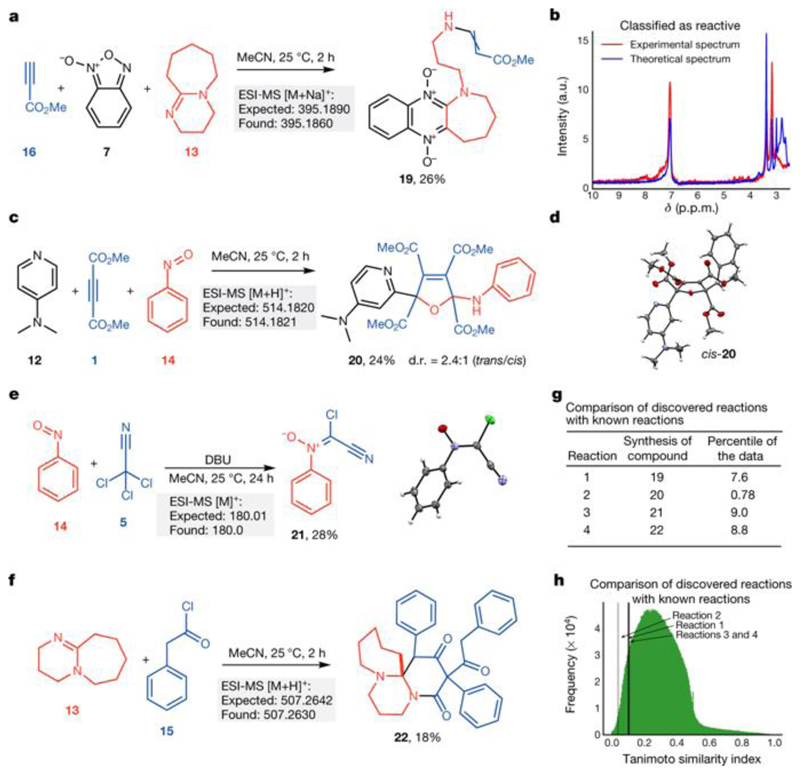
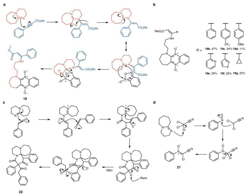
We used the reactive combinations discovered by the system to manually carry out reactions. For example, by analysing the spectra recorded by the robot, we identified several transformations (Fig. 5). For instance, analysis of the 1H NMR spectrum for the reaction of methyl propiolate (16) with benzofuroxan (7) and DBU (13) suggests an interesting transformation with new peaks visible in the chemical shift range δ = 4.0–5.0 p.p.m. and 7.9–8.5 p.p.m. (Fig. 5b). Isolation and NMR analysis of the reaction product showed that it contained protons originating from all starting materials suggesting that the compound resulted from a multicomponent reaction. Analysis of the 1H–13C heteronuclear single-quantum and multiple-bond correlation spectra determined the structure of product 19 (see Extended Data Fig. 2a for a proposed mechanism).

Fig. 5. Reactivity discovered with the machine-learning-driven robot.

a, Multicomponent reactions between methyl propiolate (16), benzofuroxan (7) and DBU (13); the yield obtained is given in per cent. Light-grey boxes show calculated and measured (by electrospray ionization mass spectroscopy, ESI-MS) molecular ion masses. b, ¹H NMR spectrum recorded in the platform for the reaction shown in a. c, Multicomponent reaction of DMAP (12), DMAD (1) and nitrobenzene (14), leading to the derivative 2,5-dihydrofuran (20). d.r., diastereometric ratio. d, Solid-state structure of compound cis-20 (50% probability level). e, Synthesis of chlorocyanonitrone (21) from nitrosobenzene (14) and trichloroacetonitrile (5) in the presence of DBU (13). f, Newly discovered reaction of phenylketene with DBU. g, Tanimoto similarity between discovered reactions and 3.5 million known reactions. h, Histogram showing the Tanimoto similarity index between the discovered reactions and 3.5 million known reactions.

We explored the utility of this reaction by synthesizing a small library of related molecules. By using substituted alkynes, we were able to prepare six structurally diverse compounds in one step (Extended Data Fig. 2b). Reaction of DMAD (1), nitrosobenzene (14) and DMAP (12) led to a multicomponent reaction with formation of 2,5-dihydrofurane derivative 20 at a diastereometric ratio of 2.4:1 (trans:cis) (Fig. 5c, d). Figure 5e shows the formation of chlorocyanonitrone 21—an unreported class of nitrones—which was isolated as the product of the reaction between trichloroacetonitrile (5) and nitrosobenzene (14) in the presence of DBU (13) (structure of 21 confirmed by X-ray analysis). Finally, we also found reactivity between ketenes and DBU (Fig. 5f), indicated by the peaks at high molecular weight recorded by the platform for this reaction (mass-to-charge ratio, m/z = 506.9 and m/z = 657); see Fig. 5f. Under basic conditions, phenylacetyl chloride (15) is deprotonated by DBU, giving phenyl ketene, which reacts with DBU to give the polycyclic azepine derivative 22 (Fig. 5f). The suggested mechanisms for these transformations are presented in Extended Data Fig. 2c, d.

To assess how unique these reactions are, we employed the Tanimoto similarity index, which compares starting materials and products. We considered over 40 million reactions, filtered by first excluding non-organic reactions, then requiring the same number of reagents and products as our discoveries, and finally by requiring that the reactions have all the necessary structural information. This filtering left more than about 3.5 million reactions to compare. For each reaction, we calculated the similarity between each reagent and the product and calculated the mean from the obtained values. For reactions in which the reagents undergo a slight modification to reach the product, this reaction similarity index would be close to 1. Conversely, if the reagents change substantially so that the product is very different, then the result would be close to 0. All four of the reactions discovered here (see Supplementary Information) have a lower similarity index than the mean. In fact, all are in the top 10 percentile, with reaction 2 (which gives product 20) in the top 0.8 percentile (Fig. 5g), and they are considerably more distinct from the reactions chosen at random. The histogram in Fig. 5h shows that there is only one peak in the distribution and that the mean value of the Tanimoto similarity index is 0.29.

This study represents an important step towards developing intelligent automated approaches to chemical discovery using artificial-intelligence-driven chemical robots trained by human experts from the bottom up, in contrast to top-down fragment-based approaches²³.

Methods

General experimental remarks

Reagents were from Sigma Aldrich and were used as received. Acetonitrile employed as a solvent in the platform was HPLC grade (VWR International). Mass spectra were recorded on a time-of-flight mass spectrometer (MicroTOF-Q MS) equipped with an electrospray source supplied by Bruker Daltonics Ltd. All data were collected in positive ion mode. The spectrometer was calibrated with a standard tune mix to give a precision of about 1.5 p.p.m. in the region m/z = 100–3,000. NMR data were recorded using a Bruker Avance III 600 MHz or a Bruker Avance 400 MHz NMR system. The spectra were recorded at 298 K using residual-solvent proton peaks for scale reference (for example, 1H: δ (CDCl3) = 7.26; 13C: δ (CDCl3) = 77.16). The chemical shifts are reported in p.p.m. using the δ scale and all coupling constants (J) are given in Hz. The following abbreviations are used to characterize spin multiplicities: s, singlet; d, doublet; t, triplet; q, quadruplet; m, multiplet; dd, double doublet; dt, double triplet; dq, double quadruplet; and ddt, double doublets of triplets. Spectra obtained using distortionless enhancement by polarization transfer, correlation spectroscopy, heteronuclear single-quantum and multiple-bond correlation spectroscopy and rotating frame Overhauser-effect spectroscopy were used for structure determination and structural assignments. New reaction candidates were analysed using thin-layer chromatography (TLC) and visualized using TLC plates with a fluorescent indicator.

Syringe pumps and tubing

Control over the fluids was achieved using 27 pumps (model C3000, Tricontinent) equipped with 5 ml syringes (TriContinent) and a four-way solenoid valve according to the requirements of the experiments. The pumps were connected using a RS232 port and a daisy chain, allowing the connection of up to 16 pumps on a single RS232 bus. Commands to the pumps were sent using the pumps’ proprietary control language, implemented in a Python module, allowing control over the pumps and error-reporting functionality (for example, pumps malfunctioning). PTFE plastic tubing with an outer diameter of 1/8 inch (3.175 mm) was cut to the specified length and connected using standard HPLC low-pressure PTFE connectors and PEEK manifolds (supplied by Kinesis).

Online attenuated total-reflectance infrared spectroscopy

All spectra were recorded using a Thermo ScientificNicoletiS5 Fourier transform infrared spectroscopy system equipped with a ZnSe Golden Gate attenuated total reflectance infrared flow cell. The resolution was set at 4 cm⁻¹ and each sample’s spectrum was recorded using 36 scans. The spectrometer was controlled by OMNIC software using Python and the ActiveX software framework. Before measurement of the spectra, the solvent (MeCN) was recorded as background.

Online NMR spectroscopy

The NMR spectra were recorded using a Spinsolve benchtop NMR system from Magritek with a compact permanent magnet (43 MHz) based on the Hallbach design, working on a lock-free basis (not requiring deuterated solvents). Shimming was performed using a D2O/H2O mixture (9:1 v:v) to minimize the half-width of the solvent peak. To measure reaction mixtures, the spectrometer was equipped with a home-built flow cell with a standard 5 mm width to maximize sensitivity. The spectra were measured in a stopped flow by pumping reaction mixtures into the flow cell. The spectrometer was controlled by Spinsolve software by sending XML messages over a network connection.

Benchtop mass spectroscopy

The spectra were recorded with an Advion Expression mass spectrometer using the atmospheric pressure chemical ionization technique. The detailed acquisition parameters can be found in Supplementary Information. The mass spectrometer was controlled using Python wrapper software and Advion API, allowing complete control over the instrument and acquisition parameters. Dilution of the reaction mixtures, which was necessary for recording their spectra, was realized using two syringe pumps by diluting reaction mixtures 3,125 times using solvent (MeCN) before the measurements.

Flow setup implementation

The platform was assembled as in Fig. 1a, using the 27 syringe pumps, the benchtop infrared spectroscopy system, the NMR and the mass spectrometer. Round bottom flasks (25 ml) were employed as the mixer and reactors. 18 pumps were responsible for dispensing the chemicals to the mixer, six pumps were used to transfer the reaction mixture from the mixer to the proper reactor, one pump was employed to pump the solvent (MeCN), and two pumps were used to realize the dilution step that was necessary to measure mass spectra. The starting materials were prepared as 1.0 M solutions. Automatic data collection and processing and platform control were achieved using the Python programming language. Before the execution of the reaction, the robot was cleaned three times by flushing the mixer, reactor flasks and analytics. The reaction was performed by adding proper reagents to the mixer (total volume 5.0 ml) in a 1:1 ratio, transferring the reaction mixture to the reactor and saving the reaction parameters (the identity and volumes of the starting materials). After two hours, the reaction mixture was transferred to the measurement loop, where the NMR and infrared spectra were recorded. The mass spectrum was recorded after dilution of the reaction mixture. After the reaction mixture has been measured, the mixer, reactor and analytics were cleaned by flushing with solvent twice. Parallel execution of six reactions was implemented by shifting the execution of each reaction in time so that each experiment had access to the liquid-handling robot and analytics without colliding with the other experiments. Spectra (NMR and infrared) were also recorded for each chemical in the pool of starting materials (Extended Data Fig. 1) that was used for the calculation of the theoretical spectrum of the reaction mixture.

Autonomous navigation of chemical space by the robot

The algorithm for the exploration of chemical space starts by measuring 90 random experiments in the platform, and then each experiment in this set is processed to assess its reactivity and generate its vector representation. The 1H NMR spectrum of the reaction mixture is automatically processed using fast Fourier transform, phasing and referencing of the solvent peak. The intensity of the solvent peak is normalized to 1.0 (the solvent peak is used as an internal standard, allowing easy addition of the spectra). The infrared spectra are used without any preprocessing. Next, the theoretical spectra of the reaction mixture (the sum of the starting materials) are constructed for NMR and infrared spectroscopy. The spectra are normalized by removing the mean and scaled to unit variance. The reactivity of the reaction mixture is assessed by feeding the NMR reaction mixture and NMR theoretical spectrum to the SVM classifier (trained previously; see Supplementary Information). The outcome of the classifier is Y = 0 (non-reactive) or Y = 1 (reactive). Similarly, the reactivity is assessed by the SVM classifier using the infrared spectra. An experiment is classified as reactive if any of the above classifiers categorizes it as reactive. The vector representation is generated using the identity of the starting materials. The vector representation (X) and reactivity (Y) are added to the reaction database.

The machine learning algorithms are realized using the sci-kit learn package in Python. After the initial database of the reactions is built, the LDA classifier is trained on the vector representation of the reactions (X) and their reactivity (Y). All the possible unperformed reactions are then rated by assigning them the probability of being reactive, as calculated from the LDA model. After the reactions with the highest score are realized by the liquid-handling robot, they are processed as described above, updating the reaction database. Then, the LDA model is retrained on the updated database and the robot iteratively explores the chemical space until the desired number of experiments is performed. Simulations of the exploration of the chemical space with this algorithm were performed using the data collected by the robot.

Syntheses of molecules discovered by the platform

The solutions of the starting materials (1.0 M solutions in MeCN) were added to the round bottom flask (25 ml) in a 1:1 ratio (total volume 5.0 ml) and stirred in room temperature for 2 h. Subsequently, silica gel (4.0 g) was added and the solvent was evaporated. The products of the reaction were isolated using column chromatography. The syntheses of all compounds were adjusted according to the need for each reaction. For the detailed procedure followed for each compound and characterization, see Supplementary Information.

Extended Data

Extended Data Fig. 1. Reaction space explored.

The chemical inputs (1–18) used in the platform to search for new transformations and to evaluate the performance of the algorithm.

Extended Data Fig. 2. Suggested mechanisms for observed transformations and small library of compounds synthesized.

a, Suggested mechanism for the synthesis of compound 19. b, Small library of compounds synthesized. c, Suggested mechanism for the synthesis of compound 22. d, Suggested mechanism for the synthesis of compound 21.

References

- 1.Collins KD, Gensch T, Glorius F. Contemporary screening approaches to reaction discovery and development. Nat Chem. 2014;6:859–871. doi: 10.1038/nchem.2062. [DOI] [PubMed] [Google Scholar]
- 2.Warr WA. A short review of chemical reaction database systems, computer-aided synthesis design, reaction prediction and synthetic feasibility. Mol Inform. 2014;33:469–476. doi: 10.1002/minf.201400052. [DOI] [PubMed] [Google Scholar]
- 3.Plata RE, Singleton DA. A case study of the mechanism of alcohol-mediated Morita Baylis-Hillman reactions. The importance of experimental observations. J Am Chem Soc. 2015;137:3811–3826. doi: 10.1021/ja5111392. [DOI] [PMC free article] [PubMed] [Google Scholar]
- 4.LeCun Y, Bengio Y, Hinton G. Deep learning. Nature. 2015;521:436–444. doi: 10.1038/nature14539. [DOI] [PubMed] [Google Scholar]
- 5.Jordan MI, Mitchell TM. Machine learning: trends, perspectives, and prospects. Science. 2015;349:255–260. doi: 10.1126/science.aaa8415. [DOI] [PubMed] [Google Scholar]
- 6.Raccuglia P, et al. Machine-learning-assisted materials discovery using failed experiments. Nature. 2016;533:73–76. doi: 10.1038/nature17439. [DOI] [PubMed] [Google Scholar]
- 7.Graulich N, Hopf H, Schreiner PR. Heuristic thinking makes a chemist smart. Chem Soc Rev. 2010;39:1503–1512. doi: 10.1039/b911536f. [DOI] [PubMed] [Google Scholar]
- 8.Gil Y, Greaves M, Hendler J, Hirsh H. Amplify scientific discovery with artificial intelligence. Science. 2014;346:171–172. doi: 10.1126/science.1259439. [DOI] [PubMed] [Google Scholar]
- 9.Trobe M, Burke MD. The molecular industrial revolution: automated synthesis of small molecules. Angew Chem Int Ed. 2018;57:4192–4214. doi: 10.1002/anie.201710482. [DOI] [PMC free article] [PubMed] [Google Scholar]
- 10.Ley SV, Fitzpatrick DE, Ingham RJ, Myers RM. Organic synthesis: march of the machines. Angew Chem Int Ed. 2015;54:3449–3464. doi: 10.1002/anie.201410744. [DOI] [PubMed] [Google Scholar]
- 11.Sans V, Cronin L. Towards dial-a-molecule by integrating continuous flow, analytics and self-optimisation. Chem Soc Rev. 2016;45:2032–2043. doi: 10.1039/c5cs00793c. [DOI] [PMC free article] [PubMed] [Google Scholar]
- 12.Houben C, Lapkin AA. Automatic discovery and optimization of chemical processes. Curr Opin Chem Eng. 2015;9:1–7. [Google Scholar]
- 13.Sans V, Porwol L, Dragone V, Cronin L. A self optimizing synthetic organic reactor system using real-time in-line NMR spectroscopy. Chem Sci. 2015;6:1258–1264. doi: 10.1039/c4sc03075c. [DOI] [PMC free article] [PubMed] [Google Scholar]
- 14.Dragone V, Sans V, Henson AB, Granda JM, Cronin L. An autonomous organic reaction search engine for chemical reactivity. Nat Commun. 2017;8 doi: 10.1038/ncomms15733. 15733. [DOI] [PMC free article] [PubMed] [Google Scholar]
- 15.Cortes C, Vapnik V. Support vector networks. Mach Learn. 1995;20:273–297. [Google Scholar]
- 16.Gómez-Bombarelli R, et al. Automatic chemical design using a data-driven continuous representation of molecules. ACS Cent Sci. 2018;4:268–276. doi: 10.1021/acscentsci.7b00572. [DOI] [PMC free article] [PubMed] [Google Scholar]
- 17.Bengio Y, Courville A, Vincent P. Representation learning: a review and new perspectives. IEEE Trans Pattern Anal. 2013;35:1798–1828. doi: 10.1109/TPAMI.2013.50. [DOI] [PubMed] [Google Scholar]
- 18.Coomans D, Jonckheer M, Massart DL, Broeckaert I, Blockx P. Application of linear discriminant analysis in the diagnosis of thyroid diseases. Anal Chim Acta. 1978;103:409–415. [Google Scholar]
- 19.Perera D, et al. A platform for automated nanomole-scale reaction screening and micromole-scale synthesis in flow. Science. 2018;359:429–434. doi: 10.1126/science.aap9112. [DOI] [PubMed] [Google Scholar]
- 20.Ahneman DT, Estrada JG, Lin S, Dreher SD, Doyle AG. Predicting reaction performance in C-N cross-coupling using machine learning. Science. 2018;360:186–190. doi: 10.1126/science.aar5169. [DOI] [PubMed] [Google Scholar]
- 21.Nielsen MK, Ahneman DT, Riera O, Doyle AG. Deoxyfluorination with sulfonyl fluorides: navigating reaction space with machine learning. J Am Chem Soc. 2018;140:5004–5008. doi: 10.1021/jacs.8b01523. [DOI] [PubMed] [Google Scholar]
- 22.Bajusz D, Racz A, Heberger K. Why is Tanimoto index an appropriate choice for fingerprint-based similarity calculations? J Cheminform. 2015;7:20. doi: 10.1186/s13321-015-0069-3. [DOI] [PMC free article] [PubMed] [Google Scholar]
- 23.Palazzolo AME, Simons CLW, Burke MD. The natural productome. Proc Natl Acad Sci. 2017;114:5564–5566. doi: 10.1073/pnas.1706266114. [DOI] [PMC free article] [PubMed] [Google Scholar]
- 24.Pedregosa F, et al. Scikit-learn: machine learning in Python. J Mach Learn Res. 2011;12:2825–2830. [Google Scholar]
Associated Data
This section collects any data citations, data availability statements, or supplementary materials included in this article.