A dual modeling approach to automatic segmentation of cerebral T2 hyperintensities and T1 black holes in multiple sclerosis

Abstract

Background and purpose

Magnetic resonance imaging (MRI) is crucial for in vivo detection and characterization of white matter lesions (WML) in multiple sclerosis (MS). The most widely established MRI outcome measure is the volume of hyperintense lesions on T2-weighted images (T2L). Unfortunately, T2L are non-specific for the level of tissue destruction and show a weak relationship to clinical status. Interest in lesions that appear hypointense on T1-weighted images (T1L) (“black holes”) has grown because T1L provide more specificity for axonal loss and a closer link to neurologic disability. The technical difficulty of T1L segmentation has led investigators to rely on time-consuming manual assessments prone to inter- and intra-rater variability. This study aims to develop an automatic T1L segmentation approach, adapted from a T2L segmentation algorithm.

Materials and methods

T1, T2, and fluid-attenuated inversion recovery (FLAIR) sequences were acquired from 40 MS subjects at 3 Tesla (3 T). T2L and T1L were manually segmented. A Method for Inter-Modal Segmentation Analysis (MIMoSA) was then employed.

Results

Using cross-validation, MIMoSA proved to be robust for segmenting both T2L and T1L. For T2L, a Sørensen-Dice coefficient (DSC) of 0.66 and partial AUC (pAUC) up to 1% false positive rate of 0.70 were achieved. For T1L, 0.53 DSC and 0.64 pAUC were achieved. Manual and MIMoSA segmented volumes were correlated and resulted in 0.88 for T1L and 0.95 for T2L. The correlation between Expanded Disability Status Scale (EDSS) scores and manual versus automatic volumes were similar for T1L (0.32 manual vs. 0.34 MIMoSA), T2L (0.33 vs. 0.32), and the T1L/T2L ratio (0.33 vs 0.33).

Conclusions

Though originally designed to segment T2L, MIMoSA performs well for segmenting T1 black holes in patients with MS.

Highlights

• •MIMoSA is an automatic T2 hyperintense lesion segmentation algorithm that can be applied to segment T1 hypointense lesions.
• •MIMoSA is the first cross validated approach for automatically segmenting T1 hypointense lesions accurately.
• •Correlations between clinical variables and MIMoSA volumes are as good or better than correlations using manual volumes.

1. Introduction

Multiple sclerosis (MS) is an inflammatory and demyelinating autoimmune disease of the central nervous system which typically leads to neurodegeneration (Ahlgren et al., 2011; Compston and Coles, 2002; Harbo et al., 2013). The inflammatory and demyelinating process causes multifocal lesions and widespread atrophy in white and gray matter, often leading to physical disability, cognitive dysfunction, and unemployment (Rovira and León, 2008; Tauhid et al., 2015). Structural magnetic resonance imaging (MRI) is a commonly used tool for the diagnosis, longitudinal management, and scientific investigation of MS (Lublin et al., 2014) because it allows for the detection of white matter lesions (WML). Common MRI metrics used to assess disease activity and severity in patient management and clinical trials include WML count and volume, the latter of which particularly relies on accurate segmentation.

Several complementary characterizations of WML are commonly delineated. Gadolinium-enhancing lesions (EL) are closely linked to acute perivascular inflammatory activity due to focal break-down of the blood-brain barrier and typically fade over 2–6 weeks (Zivadinov and Bakshi, 2004). T2 hyperintense lesions (T2L), which typically start as EL but later remain as non-enhancing lesions, are nonspecific for the severity of underlying pathology (Zivadinov and Bakshi, 2004). That is, T2 sequences are nonspecific for the type and degree of tissue injury such as demyelination, inflammation, edema or axonal loss. This nonspecificity is one factor that contributes to modest associations between T2L metrics and clinical status (Molyneux et al., 2000). Approximately 50% of T2L also appear as persistent T1 hypointensities (T1L), commonly referred to as black holes, which are likely to be the most destructive regions with severe demyelination and axonal loss (Katdare and Ursekar, 2015; Andermatt et al., 2017). Furthermore, the T1L/T2L ratio, an index of the destructive potential of lesions, has been shown to be particularly sensitive in tracking MS therapeutic response (Kim et al., 2016). T1L metrics provide high clinical significance but are usually assessed manually in both clinical and trial settings because they are difficult to segment (Bakshi et al., 2005).

Manual segmentation is the gold standard approach for WML quantification and requires an expert to analyze scans visually. Unfortunately, this process is costly, time-consuming, and prone to intra- and inter-rater variability (Lladó et al., 2012; Sweeney et al., 2014; García-Lorenzo et al., 2013). Difficulties associated with manual lesion segmentation have led to the development of various segmentation methods with different levels of accuracy and complexity (Sweeney et al., 2014). While many methods are available, no single approach has been shown to perform optimally across multiple lesion assessments and scanning platforms. This is largely due to the challenges associated with heterogeneous lesion characteristics within and across subjects and variability introduced by scanning hardware and acquisition protocols.

The majority of automatic lesion segmentation methods delineate T2L (García-Lorenzo et al., 2013; Valcarcel et al., 2018; Sweeney et al., 2013; Meier et al., 2017; Shiee et al., 2010; Dadar et al., 2017). In contrast, few studies have investigated a fully automatic segmentation approach for T1L. The sparsity of prior research is in part due to a technical challenge: since T1L and their boundaries appear similar to gray matter (Ceccarelli et al., 2012) and are subtler than the boundaries of T2L, they are much more difficult to segment by manual and automatic methods. Related to the segmentation of T1L, Khayati et al. proposed a method to segment different stages of lesions, including chronic lesions which include T1L as well as other lesional phenotypes (Khayati et al., 2008). The simplest method to segment T1L was proposed by Filippi et al. using an expert-driven semi-automated thresholding approach to estimate lesion volumes (Filippi et al., 1996). Molyneux et al. similarly proposed a semi-automated technique to delineate T1L in a multi-center study where they showed that T1L volume is a consistent and reproducible metric that can be applied to MRI data from various scanners (Molyneux et al., 2000). Following these results, Datta et al. recently developed fully automated methods using fuzzy connectivity modeling (Datta et al., 2006). Wu et al. proposed an algorithm to detect EL, T1L, and T2L using intensity-based statistical k-nearest neighbor classification combined with template-driven segmentation and partial volume artifact correction (Wu et al., 2006). To automatically segment T1L, Spies et al. proposed an approach that used a standard classification algorithm to partition T1-weighted images into gray matter, white matter, and cerebrospinal fluid and then found T1L in the white matter using voxel-wise testing with healthy controls as a reference (Spies et al., 2013). Harmouche et al. proposed a method to segment T1L and T2L jointly by modeling the posterior probability density function (Harmouche et al., 2015).

Unfortunately, none of these approaches provide publicly available software, and the studies were based on relatively small MRI datasets with uniform patient demographics and lesion load (Molyneux et al., 2000; Filippi et al., 1996; Datta et al., 2006; Wu et al., 2006; Spies et al., 2013). Additionally, studies to date have only used a single rater for manual segmentations. Likely due to these limitations, adoption of these previously published methods has been slow, and studies have continued to obtain T1L segmentations manually. A comprehensive, automated technique with readily available software that integrates aspects of WML burden of multiple lesion characterizations in a diverse patient population would thus address an important, unmet need in the radiological assessment of MS lesions.

In our previous work, a Method for Inter-Modal Segmentation Analysis (MIMoSA) was developed and validated as an automatic T2L segmentation method in people with MS. (Valcarcel et al., 2018) MIMoSA has readily available software for implementation in R as a package on Neuroconductor (https://neuroconductor.org/package/details/mimosa) with documentation and a vignette available on GitHub (https://github.com/avalcarcel9/mimosa/blob/master/vignettes/mimosa_git.md) (Valcarcel, 2018; Muschelli et al., 2018). In the present study, we applied the MIMoSA method to automatically segment T1L. Since no publicly available software for automatic detection of T1L exists, we automatically segmented T2L using MIMoSA and used these measures as a reference for T1L performance. This was motivated by our findings that MIMoSA is a competitive T2L segmentation approach (Valcarcel et al., 2018), and all T1L are also seen as T2L (but not vice-versa). Moreover, since the data in this study were acquired under a different protocol than data in the original development of MIMoSA, application of MIMoSA to segment T2L enabled us to validate and assess the robustness of MIMoSA's accuracy across different scanner platforms and protocols. For further comparison, OASIS, another validated T2L lesion segmentation algorithm (Sweeney et al., 2013), was used to automatically segment T1L. Finally, we examined correlations between lesion volume and clinical status measurements in order to determine if automatic lesion segmentation reduced noise and revealed stronger associations with disability.

Here we propose an automatic approach to segmenting T1L with software that is publicly available for implementation. The ability to segment T1L automatically and quickly has the potential to facilitate tracking of disease activity and lesional damage over time. Additionally, using the same automatic approach to determine T2L and T1L reduces variability in segmentation metrics by eliminating multiple data processing pipelines.

2. Materials and methods

2.1. Patients and study design

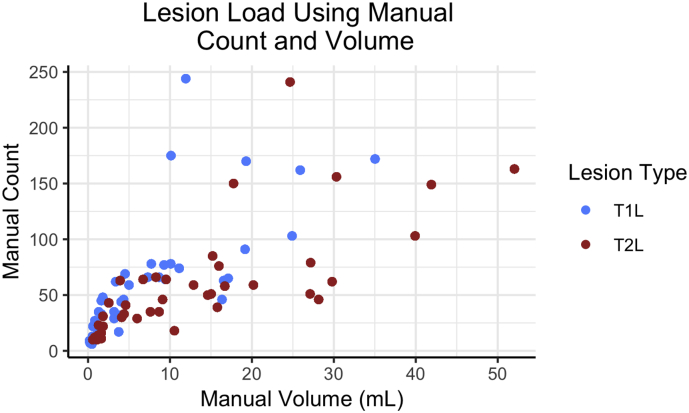
Data were collected at the Brigham and Women's Hospital in Boston, Massachusetts. The Institutional Review Board approved the study and transfer of data to the University of Pennsylvania. Forty patients, all with a clinical diagnosis of MS, were consecutively obtained from MRI scans at the center. Subjects had an examination by an MS specialist neurologist to assess the type of MS, the level of physical disability on the Expanded Disability Status Scale (EDSS), and ambulatory function on the timed 25-ft walk (T25FW). Patient demographics are provided in Table 1. Additionally, a scatterplot of lesion count against volume is displayed in Fig. 1, which shows a wide range of lesion counts and volumes across subjects.

Table 1.

Demographic information for subjects in this study are provided. Included were 40 subjects diagnosed with multiple sclerosis (MS) and scanned between 2015 and 2016 at the Brigham and Women's Hospital.

a	Mean	Std. Dev.	Min, Max
Age (years)	50.4	9.9	30.4, 69.9
Disease duration (years)	14.5	4.6	3.8, 21.3
Expanded Disability Status Scale score	2.3	1.6	0, 7
Timed 25-ft walk (seconds)	5.1	2.6	3.0, 18.4
T1L manual volume	7.70	8.33	0.18, 35.03
T2L manual volume	13.57	12.78	0.58, 52.04

b	%
Male	30
Female	70
Relapsing-Remitting MS	80
Secondary Progressive MS	20

Fig. 1.

Lesion volume (mL) and count for each subject are presented using manual segmentation masks. The lesion number and volume across subjects are both diverse for T1 lesions (T1L) and T2 lesions (T2L).

2.2. Image acquisition and preprocessing

High-resolution 3D T1-weighted (T1WI), T2-weighted (T2WI), and fluid-attenuated inversion recovery (FLAIR) volumes of the brain were collected on a Siemens 3 Tesla (3 T) Skyra instrument using a consistent scan protocol for all subjects. Acquisition details are provided in Table 2 and have also been detailed previously (Meier et al., 2017).

Table 2.

Image acquisition protocol using a 3 Tesla (3 T) Siemens Skyra scanner at the Brigham and Women's Hospital.

3 T Brain MRI Acquisition Protocol
Scanner Hardware	Siemens Skyra
Scanner Software	Syngo MR D13
Coil	20 channel
MR Acquisition Type	3D
Orientation	Sagittal
Number of signal averages	1
Sequence type	FLAIR	T2WI	T1WI
Number of slices	176	192	176
Voxel size (mm)	1.0 × 1.0 × 1.0	0.98 × 0.98 × 1.0	1.0 × 1.0 × 1.0
TR (ms)	5000	2500	2300
TE (ms)	389	300	2.96
TI (ms)	1800	N/A	900
Flip angle (degrees)	120	120	9
Parallel acceleration	2	4	2
Scan time (minutes)	6:00	3:18	5:09

All images were preprocessed prior to implementing the MIMoSA model using the R (version 3.1.0, R Foundation for Statistical Computing, Vienna, Austria) packages extrantsr (Muschelli, 2017) and WhiteStripe (Shinohara and Muschelli, 2017), as well as Multi-Atlas Skull-Stripping (MASS) (Doshi et al., 2013; NITRC, n.d.). After N4 inhomogeneity correction (Tustison et al., 2010), volumes were co-registered across sequences for each subject using a rigid-body transformation with a Lanczos windowed sinc interpolator. To remove extracerebral voxels, MASS was implemented (Doshi et al., 2013; NITRC, n.d.). Manually delineated T2L masks were obtained in the FLAIR space, and manual T1L masks were obtained in the T1WI space. To avoid interpolation errors in these masks, analyses of T1L and T2L were conducted in their respective native spaces and no transformations of the segmentation masks nor the primary imaging sequences were applied. First, T1WI and T2WI images were registered to the FLAIR for all T2L modeling; then, separately, T2WI and FLAIR images were registered to the T1WI space for all T1L modeling. As conventional MRI volumes are acquired in arbitrary units, statistical intensity normalization using WhiteStripe (Shinohara and Muschelli, 2017) was applied in order to facilitate modeling of intensities across subjects.

2.3. Image analysis

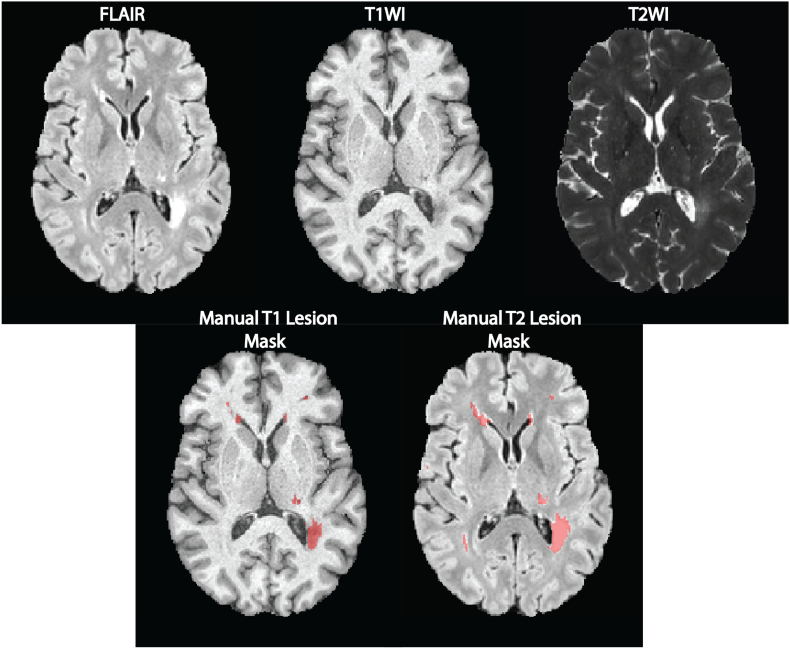
T1L and T2L were manually segmented by a reading panel of two trained observers under the supervision of an experienced observer at the Brigham and Women's Hospital. Each trained observer independently determined the presence or absence of T1L and T2L and then reviewed these results together to form a consensus. In the event of a disagreement, a senior experienced observer was consulted. A WML was categorized as a T2L if it appeared as hyperintense on the FLAIR. T1L, or black holes, were defined as appearing hypointense on T1WI and at least partially hyperintense on the FLAIR volumes. After a consensus of lesions was determined, one observer segmented all T1L and T2L using an edge-finding tool in Jim (v. 7.0) (Internet Analysis Tools Registry, n.d.). This process resulted in manually segmented gold standard masks for T1L and T2L for each subject in the study. Fig. 2 shows examples of preprocessed images and manual T1L and T2L segmentations. All gadolinium-enhancing lesions were excluded from T1L manual segmentations.

Fig. 2.

Axial slices from an inhomogeneity corrected, registered, and intensity normalized MRI of a single subject are displayed in the top row. In the bottom row, manual lesion segmentation masks are overlaid on T1WI and FLAIR volumes.

2.4. Automatic segmentation of T1L and T2L using MIMoSA

2.4.1. Overview

To automatically segment both T1L and T2L, MIMoSA (Valcarcel et al., 2018) was applied using the mimosa (Valcarcel, 2018) package in R, which is available on Neuroconductor (Muschelli et al., 2018). MIMoSA was originally developed to automatically segment T2L. We attempted to modify the MIMoSA paradigm to better tailor it to the T1L segmentation task by introducing: 1) a two-stage model that first segments T2L and then segments T1L, and 2) a modification of the candidate mask procedure. However, these changes did not improve the results over the original MIMoSA method proposed for T2L segmentation. Therefore, the original method was applied with no changes. In this section, we broadly summarize the steps of the approach and elaborate on each step in the sections that follow.

MIMoSA relies on a brain tissue mask that excludes cerebrospinal fluid and extracerebral tissue. Given this mask, MIMoSA first identifies candidate lesion voxels by thresholding hyperintensities on the FLAIR. This step reduces computation time and minimizes false positive detection. Since feature extraction is known to be pivotal for a segmentation algorithm's accuracy and generalizability (Sweeney et al., 2014), MIMoSA relies on features that capture the mean structure of each imaging volume as well as the covariance across volumes. The procedure proceeds by creating these features, which are later used as predictors in a multivariable regression model. Once all relevant features have been calculated, MIMoSA fits a local logistic regression using training data with gold standard manual segmentations of either T1L or T2L. Coefficients from the model fit are then used to produce maps that contain the probability that each voxel location contains lesional tissue. Thresholding can be applied to the probability maps to obtain binary lesion segmentation maps for each patient. MIMoSA also includes a thresholding algorithm that optimizes the similarity of predicted segmentation masks in the training set with manual segmentations based on the Sørensen-Dice coefficient (DSC). The MIMoSA model can then be applied to subjects who were not included in the training set in order to automatically segment lesions.

In this study, MIMoSA was applied to automatically segment T1L and T2L by fitting separate models for each lesion type. One model was fit to segment T2L using preprocessed images registered to the FLAIR space, and a separate model was fit to segment T1L using preprocessed images registered to the T1WI space. This separate fitting procedure is necessary because, while all T1L are seen as T2L, not all T2L are seen as T1L (Sweeney et al., 2014). Specific steps of the MIMoSA method are described in more detail in the following sections and illustrated in Fig. 3.

Fig. 3.

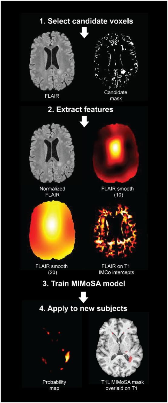
The MIMoSA procedure is demonstrated and visualized in an example axial slice. 1. MIMoSA first selected candidate voxels defined as being the 85th quantile or above in intensity on the FLAIR images. 2. Features inside the candidate mask were then extracted (full brain features derived from FLAIR volumes are only shown for simplicity). 3. To obtain T1 lesion (T1L) masks and T2 lesion (T2L) masks, separate models were fit. 4. Training the MIMoSA models on a subset of subjects with manual segmentations yielded segmentation models which were then applied to test subjects not included in the training set.

2.4.2. Candidate voxel selection

The first step in the MIMoSA procedure is to select candidate voxels for lesion presence for a candidate mask. Since WML appear as hyperintensities on the FLAIR volume, the method excludes voxels whose FLAIR intensities are likely not consistent with lesional tissue. Candidate voxels are defined as the 85th percentile and above on the FLAIR volume. This step reduces computation time and restricts the modeling space, which empirically has been found to reduce false positives and leads to an increase in performance measures (Valcarcel et al., 2018; Sweeney et al., 2013).

2.4.3. Feature extraction

The next step in the algorithm is to obtain features from the candidate voxels that will be used in the model. MIMoSA utilizes three distinct feature types: (1) normalized images, (2) smoothed images, and (3) inter-modal coupling (IMCo) intercept and slope images (Vandekar et al., 2016). MIMoSA allows for T1WI, T2WI, FLAIR, and Proton Density (PD) MRI modalities as inputs, but it has been shown that only T1WI and FLAIR sequences are required to achieve statistically equivalent performance to the model with all four sequences (Valcarcel et al., 2018). In this study, PD images were not collected; therefore, only T1WI, T2WI, and FLAIR are used as inputs and subsequently included in the model as features. Since sequences are generally acquired in arbitrary units, MIMoSA utilizes intensity-normalized images to facilitate across-subject modeling of intensities (Valcarcel et al., 2018; Sweeney et al., 2013). To account for average signal intensities around each voxel, Gaussian smoothers with varying kernel sizes are applied to the intensity-normalized images and also included in the model. The smoothed-image features have been noted to mitigate segmentation artifacts that are due to residual image inhomogeneity after N4 correction (Shinohara et al., 2011) and to incorporate local spatial context. The model incorporates images smoothed with parameters σ=10 mm and σ=20 mm. To further help distinguish the lesional tissue from normal appearing white matter, the MIMoSA model includes features extracted from IMCo regressions, which quantify the local covariance between two image modalities throughout the brain at the subject level. For a given center voxel, the IMCo features are extracted from a weighted linear regression of one modality on the other in a local neighborhood around the center voxel. The weights are derived from a Gaussian kernel with fixed full width half maximum (FWHM) parameter (3 mm). Thus, voxels in the neighborhood are weighted by their distance to the center voxel. MIMoSA estimates the intercept and slope from a weighted linear regression at all voxels in the candidate mask for each pair of imaging modalities. That is, MIMoSA exhausts all possible pairs of the scanning contrasts available for feature extraction. For each pair, IMCo regression is performed twice so that both image types in the pair are used, once as the outcome and once as the predictor. For example, for T1WI and FLAIR images, MIMoSA performs IMCo regression using T1WI intensities as the predictor with FLAIR intensities as the outcome and then repeats the IMCo regression with T1WI as the outcome and FLAIR as the predictor. With our three contrasts, six unique IMCo regressions were performed.

2.4.4. Fit the MIMoSA model

After features are calculated, a logistic regression is fit to model the probability that a voxel contains lesional tissue (Walter, 2005). Logistic regression is straightforward to interpret and implement and is commonly used in the segmentation literature (Sweeney et al., 2014; Dadar et al., 2017).

The MIMoSA model is a voxel-level logistic regression that is fit using the candidate voxels. Let L_i(v) be a random variable denoting voxel-level lesion presence at voxel v; if voxel v contains lesional tissue for subject i, then L_i(v) = 1, otherwise L_i(v) = 0. We model the probability that a voxel v contains lesion P{L_i(v) = 1} with the following logistic regression model:

$$\text{logit}\left[\mathrm{P}\left\{{\mathrm{L}}_{\mathrm{i}}\left(\mathrm{v}\right)=1\right\}\right]={\mathrm{\beta }}_0+{\mathrm{X}}_{\mathrm{i}}^{\mathrm{T}}\left(\mathrm{v}\right)\mathrm{\beta }+\mathfrak{G}{\mathrm{X}}_{\mathrm{i}}^{\mathrm{T}}\left(\mathrm{v},10\right)\left\{{\mathrm{\beta }}_{10}+{\mathrm{X}}_{\mathrm{i}}\left(\mathrm{v}\right)⨂{\mathrm{\beta }}_{10}^{\ast }\right\}\mathfrak{+}\mathfrak{G}{\mathrm{X}}_{\mathrm{i}}^{\mathrm{T}}\left(\mathrm{v},20\right)\left\{{\mathrm{\beta }}_{20}+{\mathrm{X}}_{\mathrm{i}}\left(\mathrm{v}\right)⨂{\mathrm{\beta }}_{20}^{\ast }\right\}+\mathcal{C}{\mathrm{X}}_{\mathrm{i},\mathrm{I}}^{\mathrm{T}}\left(\mathrm{v}\right){\mathrm{\beta }}_{\mathrm{I}}+\mathcal{C}{\mathrm{X}}_{\mathrm{i},\mathrm{S}}^{\mathrm{T}}\left(\mathrm{v}\right){\mathrm{\beta }}_{\mathrm{S}},$$

where we denote the normalized images by X_i(v) = [T_{1, i}(v), FLAIR_i(v), T_{2, i}(v)]^T and express the smoothed images in vector form by $\mathfrak{G}{\mathrm{X}}_{\mathrm{i}}\left(\mathrm{v},\mathrm{\delta }\right)={\left[\mathfrak{G}\left({\mathrm{T}}_{1,\mathrm{i}}\left(\mathrm{v}\right);\mathrm{N}\left(\mathrm{v},\mathrm{\delta }\right)\right),\dots \mathfrak{.},\mathfrak{G}\left({\mathrm{T}}_{2,\mathrm{i}}\left(\mathrm{v}\right);\mathrm{N}\left(\mathrm{v},\mathrm{\delta }\right)\right)\right]}^{\mathrm{T}},$ where $\mathfrak{G}$ denotes the image smoothing operator with parameter δ ∈ {10 mm, 20 mm}. We further denote all combinations of intercept and slope IMCo parameters respectively by $\mathcal{C}{\mathrm{X}}_{\mathrm{i},\mathrm{I}}^{\mathrm{T}}\left(\mathrm{v}\right)$ and$\mathcal{C}{\mathrm{X}}_{\mathrm{i},\mathrm{S}}^{\mathrm{T}}\left(\mathrm{v}\right)$. We use ⨂ to represent the Hadamard product. The interaction terms between the normalized volumes and the smoothed volumes, denoted by β_j0^∗, contribute to the model by capturing differences between voxel intensities and their local mean intensities. These aid in mitigating artifacts due to residual field inhomogeneity and have generally been shown to improve lesion detection performance (Sweeney et al., 2014; Sweeney et al., 2013).

The normalized and smoothed volumes allow the MIMoSA model to capture mean structure within modalities and the IMCo features help to capture inter-modal patterns that contain information about lesion presence. The combination of modeling mean structure within an image type and the covariance across image types allows for sensitive and specific delineation of WML. The model is trained using manually segmented gold standard lesion masks. Two separate models are fit for automatically segmenting T1L and T2L using their respective gold standard masks. More specifically, the only difference between the models is whether L_i(v) denotes T1L or T2L. Each model output is a set of coefficients that can be used to obtain lesion probability maps on subjects not included in the training of the model.

2.4.5. Apply the MIMoSA model

To determine where lesions are present, a probability map is obtained using the estimated regression coefficients for each voxel in the candidate mask. To create a binary segmentation, a population-level threshold on the probability map is applied. Any lesion smaller than 8 cubic millimeters is removed (Shinohara et al., 2011). Fig. 3 shows an example of a probability map and binary segmentation for a subject not included during training of the model.

2.4.6. Optimal thresholding algorithm

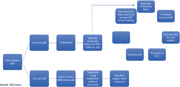
To make the method fully automated, an optimization strategy for the thresholding is employed to yield binary lesion segmentations. After the model is fit on the training data, probability maps for the subjects in the training set are generated. A threshold is then applied to the probability maps for each subject based on a user-defined grid of possible threshold values to create a set of binary segmentation masks; in this study, the grid selected was 0% to 100% by 1% increments. Using the set of predicted lesion masks for each threshold, DSC is calculated at the subject level. After DSC is calculated for each subject in the training set, the average across subjects for each threshold is collected. The threshold with the highest average DSC score is applied to probability maps estimated for subjects in the test set.

2.5. Statistical analyses

Training and testing of the MIMoSA method was conducted using cross-validation. In addition to implementing MIMoSA, a competitive T2L segmentation algorithm, OASIS was also applied (Valcarcel et al., 2018). OASIS was specifically chosen for the present study because it can be easily trained using publicly available software and there are no publicly available data for benchmarking T1L automatic lesion segmentation. To fit the models and measure performance, 100 iterations of the following procedure were performed. First, 20 subjects were randomly allocated to the training set and the remaining 20 subjects constituted the test set. Thus, every subject was represented in each iteration. MIMoSA and OASIS were then trained to detect T1L and T2L separately using subjects in the training set. After fitting the models, the estimated coefficients were applied to the test set to generate probability maps. To generate lesion masks, the threshold obtained from the optimal thresholding algorithm described above was applied.

In each of the 100 iterations, subject-level DSC, partial AUC (pAUC, up to 1% false positive rate), root mean square error (Root MSE), detection error (DE) (Wack et al., 2012), and outline error (OE) (Wack et al., 2012) were recorded (Sing et al., 2005). pAUC was estimated instead of traditional AUC because it only considers regions of the ROC space that correspond to clinically relevant values of specificity (Walter, 2005). All performance measures were calculated at the subject level and then averaged across subjects and cross-validation folds. Fig. 4 shows the full cross-validation pipeline. In addition to these summary measures, MIMoSA performance was assessed by estimating the Pearson correlation ($\widehat{\rho }$) between manually segmented and MIMoSA-predicted volumes.

Fig. 4.

Cross-validation scheme used to assess MIMoSA performance on T1 lesions (T1L) and T2 lesions (T2L) is pictured. Subjects were randomized to either the training set or the testing set. The MIMoSA model was fit using subjects in the training set. To identify the optimal threshold, probability maps were generated for subjects. These maps were thresholded along a grid selected from 0% to 100% by 1% and then the Sørensen-Dice coefficient (DSC) was calculated. The threshold that resulted in the maximum DSC across subjects in the training set was applied as the threshold in the test set. This procedure was iterated 100 times. Summary statistics are based only on the test set data. The same analysis was repeated using OASIS as the segmentation approach.

To adjudicate MIMoSA's performance, Pearson correlation coefficients were calculated to assess the relationship between image-derived features (T1L volume, T2L volume, and the T1L/T2L ratio (Kim et al., 2016)) and clinical variables, including clinical status, disease duration (time from first symptoms in years), EDSS score, and T25FW. Manual segmentation-based measures of T1L, T2L, and the T1L/T2L ratio were also computed, and associations with clinical variables were estimated for comparison. To avoid overfitting, correlations were estimated in each cross-validation fold using only subjects in the test set and then averaged across folds. We denote MIMoSA measures by $\widehat{\rho }\left(\mathit{MIMoSA}\right)$, whereas manual evaluations are represented by $\widehat{\rho }\left(\mathit{Manual}\right)$. For each measure, p-values were similarly calculated in each fold and averaged across folds. We additionally calculated each measure adjusted for sex and age.

In order to assess the accuracy and variability of the optimal threshold for each subject in the testing set we applied thresholds from 0% to 100% by 1% increments to obtain lesion masks. DSC was then calculated comparing the MIMoSA mask at each threshold with the manual segmentation.

3. Results

3.1. Segmentation Accuracy

Results are provided in Table 3, including average DSC, partial AUC with up to 1% false positive rate, and the correlation coefficient for MIMoSA and OASIS volumes with manual volumes ($\widehat{\rho }$). Results in Table 3 indicate competitive lesion segmentation performance of both T1L and T2L. DSC and pAUC for T2L lesion segmentation were competitive compared to state-of-the-art automatic methods. DSC and pAUC for T1L were modest compared to those measures for T2L but high compared with previous automated approaches in T1L studies. The MIMoSA performance measures were all greater than the OASIS performance measures, indicating superior automatic segmentation. Specifically, for T1L the 95% confidence interval for DSC was 0.02 to 0.16 and pAUC was 0.03 to 0.13. Since 0 is not contained in these intervals, we can conclude that MIMoSA statistically significantly segmented T1L more accurately than OASIS.

Table 3.

Results from the cross-validation are presented. Sørensen-Dice coefficient (DSC), partial AUC (pAUC) with up to 1% false positive rate, root mean square error (Root MSE), detection error (DE), and outline error (OE) were averaged within each testing set and then across folds. Standard deviation (SD) was calculated within cross-validation folds and then averaged across 100 iterations. DE and OE are presented in mL. The correlation coefficient relating MIMoSA volumes to manual volumes ($\widehat{\mathit{\rho }}$) was recorded in each fold and then averaged across folds.

Results
	DSC (SD)	pAUC (SD)	Root MSE (SD)	DE (SD)	OE (SD)	$\widehat{\mathrm{\rho }}$
MIMoSA T1L	0.53 (0.14)	0.64 (0.12)	0.06 (0.03)	1.02 (0.96)	9.22 (9.63)	0.88
OASIS T1L	0.43 (0.14)	0.55 (0.13)	0.08 (0.04)	1.76 (1.49)	9.85 (1.49)	0.85
MIMoSA T2L	0.66 (0.13)	0.70 (0.10)	0.07 (0.03)	1.41 (1.12)	14.9 (13.8)	0.95
OASIS T2L	0.55 (0.13)	0.62 (0.11)	0.09 (0.04)	2.55 (2.17)	15.6 (15.1)	0.88

Similarly, the DE, OE, and Root MSE were all lower for MIMoSA segmentations than OASIS, indicating that MIMoSA has less error. The DE for both methods was very small, indicating that the automatic methods detected most of the lesions that were found manually. OE was much higher than DE, indicating that the automatic methods tended to disagree at the boundary of lesions. Root MSE, though very small for both MIMoSA and OASIS, favored MIMoSA and suggested that MIMoSA had smaller average error.

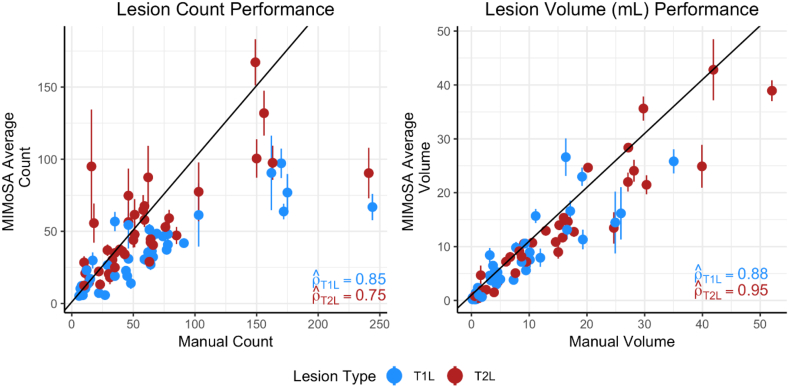
Change in lesion volume and counts are both important outcomes commonly used in MS clinical trials (Bakshi et al., 2005). The correlation between manual segmentation volume and MIMoSA volume was high for both T1L and T2L. In Fig. 5, plots of MIMoSA predicted volume are displayed against manual segmentation volume. The trend for both T1L volume and T2L volume were markedly linear and close to the identity line. Subjects with low total lesion volume tended to have accurate MIMoSA volume estimation with small variance. As total lesion volume increases, the standard deviations around the MIMoSA volume estimates increase. Fig. 5 also provides plots of MIMoSA predicted count versus manual segmentation count. The count estimated by MIMoSA for subjects with smaller lesion volumes (i.e. less than 25 mL) was similar to the manual segmentation count. For larger lesion loads, MIMoSA underestimated the count. With a few exceptions, subjects with low lesion counts tended to have small variance around the MIMoSA estimate, but variability of the estimates can be seen to increase along with increasing lesion counts. Although MIMoSA underestimated lesion count for subjects with large manual lesion counts, the MIMoSA volume estimate remained accurate. In follow-up investigations, we found that the joint underestimation of lesion count and accurate estimation of volume by MIMoSA was attributable to generous segmentation of spatially neighboring lesions that resulted in more confluent lesions.

Fig. 5.

Lesion volume and count are presented to compare manual segmentation with MIMoSA segmentation metrics. MIMoSA values were obtained by averaging volume or count for each test subject across cross-validation folds (100). The solid line depicts the y = x line. Vertical lines traversing the points are computed at the subject-level and indicate one standard deviation above and below the mean.

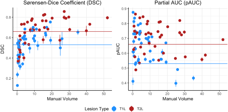
Subject-level DSC and pAUC are presented in Fig. 6. While DSC tended to be larger for patients with larger manual lesion volume, pAUC tended to be higher for patients with small to moderate manual lesion volume.

Fig. 6.

To further demonstrate model accuracy, Sørensen-Dice coefficient (DSC) and partial AUC (pAUC) with up to 1% false positive rate were calculated. Results for each subject were averaged across folds and are presented. Horizontal lines are the respective overall averages presented in Table 2. Vertical lines traversing the points are computed at the subject-level and indicate one standard deviation above and below the mean.

3.2. Correlations with clinical status

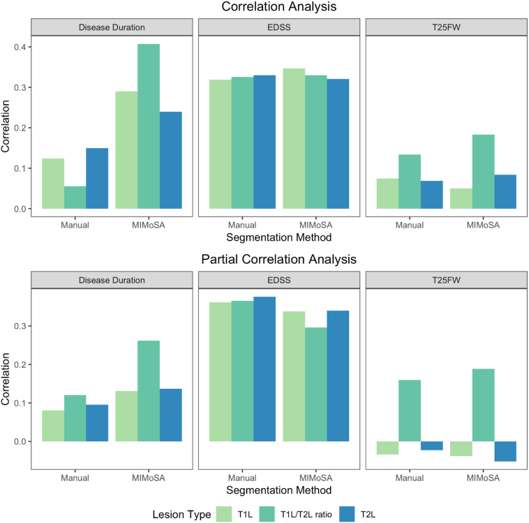
In practice, lesion segmentation metrics are commonly used to predict clinical status and evaluate therapeutic efficacy (Zivadinov and Bakshi, 2004; Bakshi et al., 2005). In Table 4, clinical measures are related to both manual and MIMoSA lesion segmentation metrics. EDSS score and T25FW were correlated with T1L and T2L volume, as well as the T1L/T2L ratio. The correlations displayed in this table show that $\widehat{\rho }\left(\mathit{MIMoSA}\right)$ tended to be equal to or larger than $\widehat{\rho }\left(\mathit{Manual}\right)$. The associated p-values in Table 4 indicate that MIMoSA and the manual segmentations performed similarly. Age and sex-adjusted results were similar to unadjusted results, with the exception of EDSS. Results are visualized in Fig. 7. The correlations, whether calculated with the manual or MIMoSA volumes, were modest but consistent with the established literature.

Table 4.

Clinical-MRI relationships with manual lesion volume, denoted as $\widehat{\rho }\left(\mathit{Manual}\right)$, or MIMoSA lesion volume, denoted as $\widehat{\rho }\left(\mathit{MIMoSA}\right)$, was averaged across cross-validation folds. T1 lesion (T1L) volume, T2 lesion (T2L) volume, and the T1L/T2L ratio were correlated separately with Expanded Disability Status Scale (EDSS) score, timed 25-ft walk (T25FW), and disease duration. For each assessment, p-values were calculated and are presented in parentheses beside each measure. The first table presents unadjusted correlations; the second table presents correlations adjusted for sex and age (in years).

Clinical Associations
		EDSS	T25FW	Disease duration
T1L	$\widehat{\rho }\left(\mathit{Manual}\right)$, (p-value)	0.32, (0.26)	−0.07, (0.56)	0.12, (0.54)
	$\widehat{\rho }\left(\mathit{MIMoSA}\right)$, (p-value)	0.34, (0.21)	−0.05, (0.58)	0.29, (0.30)
T2L	$\widehat{\rho }\left(\mathit{Manual}\right)$, (p-value)	0.33, (0.24)	−0.07, (0.55)	0.15, (0.52)
	$\widehat{\rho }\left(\mathit{MIMoSA}\right)$, (p-value)	0.32, (0.23)	−0.08, (0.56)	0.23, (0.37)
T1L/T2L ratio	$\widehat{\rho }\left(\mathit{Manual}\right)$, (p-value)	0.33, (0.22)	0.13, (0.56)	0.06, (0.54)
	$\widehat{\rho }\left(\mathit{MIMoSA}\right)$, (p-value)	0.33, (0.22)	0.18, (0.45)	0.40, (0.12)

Adjusted Clinical Associations
		EDSS	T25FW	Disease duration
T1L	$\widehat{\rho }\left(\mathit{Manual}\right)$, (p-value)	0.36, (0.23)	−0.03, (0.56)	0.08, (0.59)
	$\widehat{\rho }\left(\mathit{MIMoSA}\right)$, (p-value)	0.34, (0.25)	0.04, (0.58)	0.13, (0.53)
T2L	$\widehat{\rho }\left(\mathit{Manual}\right)$, (p-value)	0.38, (0.21)	−0.02, (0.55)	0.10, (0.57)
	$\widehat{\rho }\left(\mathit{MIMoSA}\right)$, (p-value)	0.34, (0.23)	−0.05, (0.58)	0.14, (0.50)
T1L/T2L ratio	$\widehat{\rho }\left(\mathit{Manual}\right)$, (p-value)	0.36, (0.20)	0.16, (0.53)	0.12, (0.51)
	$\widehat{\rho }\left(\mathit{MIMoSA}\right)$, (p-value)	0.30, (0.31)	0.18, (0.46)	0.26, (0.30)

Fig. 7.

Visualization of clinical-MRI relationships. Both manual and MIMoSA segmentations provided T1 lesion (T1L) volume, T2 lesion (T2L) volume, and the T1L/T2L ratio. The value of the vertical axis for disease duration, Expanded Disability Status Scale (EDSS) score, and timed 25-ft walk (T25FW) represents the Pearson correlations between each measure and the MIMoSA or manual segmentation volume. The first row presents unadjusted correlations and the second row presents correlations adjusted for sex and age (in years).

Fig. 7 also facilitates the comparison of correlations across the T1L and T2L metrics, both marginally and adjusted for age and sex. T1L and T2L tended to have similar correlations with clinical variables. However, the T1L/T2L ratio has similar or higher correlations with clinical measures. Notably, the partial correlations of T1L and T2L with T25FW are small in magnitude, whereas the T1L/T2L ratio is more strongly associated with T25FW.

3.3. Optimal threshold

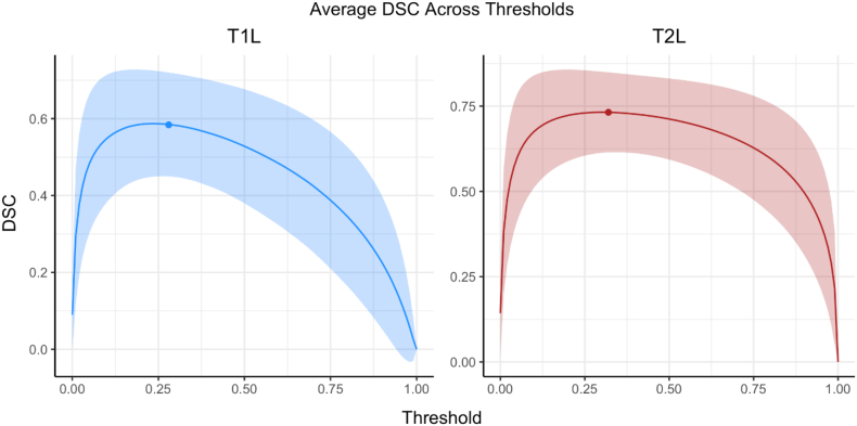
To assess the accuracy and variability of the optimal thresholding algorithm, Table 5 presents summary measures across the cross-validation iterations. The mean values were slightly larger for T2L compared to T1L, while the standard deviations and range were similar. Fig. 8 shows average DSC across thresholds applied to subjects in the testing set. For both T1L and T2L, the average optimal threshold that was applied, denoted by the colored point, lay close to the peak of each curve, which indicates that the optimal threshold algorithm indeed chose appropriate thresholds to apply to test subjects. Additionally, we note that the relatively flat areas of the curves surrounding the maximum DSC value suggest that slight differences in thresholds did not have a major impact on segmentation accuracy.

Table 5.

Summary measures for the optimal threshold obtained across iterations in the cross-validation are shown for T1 lesions (T1L) and T2 lesions (T2L).

Lesion Type	Mean	Std. Dev.	Min, Max
T1L	0.28	0.05	0.2, 0.36
T2L	0.32	0.04	0.25, 0.39

Fig. 8.

To assess the accuracy and variability of the optimal threshold, the average Sørensen-Dice coefficients (DSC) across subjects and iterations are shown across thresholds. Results for T1 lesions (T1L) and T2 lesions (T2L) are presented separately. The solid line represents the average while the filled-in area corresponds to one standard deviation from the mean. The round points on each figure are the average optimal threshold selected.

3.4. Qualitative performance

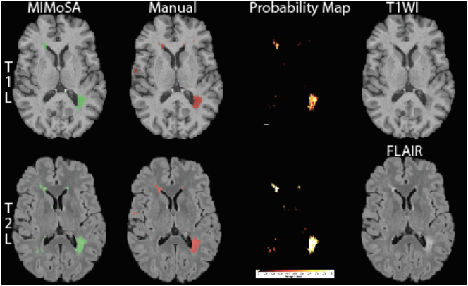
An example of MIMoSA's qualitative performance is provided in Fig. 9, where an axial slice from a subject chosen at random is provided. MIMoSA masks are overlaid on T1WI and FLAIR volumes respectively for T1L and T2L, and the probability maps used to generate MIMoSA segmentations are shown. Qualitative results were consistent with quantitative performance.

Fig. 9.

Segmented T1 lesions (T1L) and T2 lesions (T2L) in a randomly selected subject and axial slice are pictured. The first row shows T1L segmentations for both MIMoSA and manual assessment, the MIMoSA probability map, and the T1WI volume. In the second row, T2L segmentations for both MIMoSA and manual assessment, the MIMoSA probability map, and the FLAIR volume are displayed. The Sørensen-Dice coefficients (DSC) between the MIMoSA and manual segmentation for T1L and T2L were 0.54 and 0.69, respectively. To elucidate the differences between the T1L and T2L tissue type segmentations for both the MIMoSA and manual segmentations, we provide DSC between the lesion types. The DSC between MIMoSA T1L and T2L was 0.64 and the DSC between the manually segmented T1L and T2L was 0.52.

4. Discussion

MIMoSA is a fully automated segmentation method that leverages changes in inter-modal covariance structure that occurs in white matter pathology. It can be used to delineate T1L and T2L accurately, reliably, and efficiently in people with MS. Improvements in accuracy seem to be driven by the inclusion of IMCo regression features, which are features that are not included in OASIS. These measures seem especially useful for detecting T1L, a challenging task since T1L lesions often appear similar to gray matter. MIMoSA does not require human input, which promises to promote stability across a range of lesion delineation tasks. By using the same procedure to automatically segment T1L and T2L, MIMoSA also offers a consistent framework to obtain both metrics. Furthermore, the optimal thresholding algorithm fully automates the MIMoSA segmentation method by using the training subjects and their manual segmentations to provide a threshold that empirically works well in the test set. Results from our cross-validation experiments demonstrate its accuracy and support its use in practice. The MIMoSA model can easily be adapted and trained for cases with different sets of imaging sequences (Valcarcel et al., 2018; Sweeney et al., 2013). The full modeling procedure is fast and can be easily implemented using software and documentation provided on Neuroconductor (Valcarcel, 2018; Home/Neuroconductor, n.d.).

MIMoSA provides accurate and reliable automatic segmentations of both T1L and T2L. Though T2L DSC and pAUC measures were slightly larger, indicating greater similarity with our manual segmentations, T1L performance was competitive. Simultaneous delineation of T1L and T2L may lead to a better understanding of overall patient status. MIMoSA total lesion volumes were well-correlated with the manual total lesion volumes, suggesting that MIMoSA may provide a promising alternative to manual segmentation in the assessment of new therapies in clinical trials (Valcarcel et al., 2018). This may be especially useful for multi-center studies with a large number of patients or longitudinal studies with sequences collected over time.

The MIMoSA method was previously implemented on data acquired at a different site using a different scanner and acquisition protocol than data collected in this study (Sweeney et al., 2013; Valcarcel, 2018). The results here indicate that the method performed well using images acquired across scanner manufacturers and protocols when the model was appropriately trained. Previously published experiments indicate that 20 subjects is sufficient for model training (Valcarcel et al., 2018). Pre-trained models are available for immediate application of the method, but for the best results training on data acquired under the protocol of interest is encouraged (Valcarcel, 2018; Home/Neuroconductor, n.d.). The MIMoSA method should be implemented after appropriate image preprocessing. MIMoSA users should be aware that processing failures in registration, skull-stripping, and normalization may lead to segmentation failures. Quality control should be implemented after each step of preprocessing before applying MIMoSA.

Often lesion volumes are correlated with clinical covariates and disease status in patient management and clinical trials that evaluate therapy effectiveness. Therefore, automatic segmentation approaches should be as sensitive as manual measures. Correlations were provided to compare manual and MIMoSA segmentations with clinically relevant variables. Our results indicate that the relationship between MIMoSA volumetric assessments showed as close or better correlations compared to correlations with manual segmentations. This was likely due to the stability and consistency introduced by an automatic method that requires no operator input. Segmentation of T1L can be challenging since the intensity profile is often indistinguishable from gray matter (Bakshi et al., 2005), especially with respect to delineating boundaries; thus, reliability in these areas may be driving stronger correlation with covariates. For T2L evaluation, correlations seemed to be approximately equal between MIMoSA and manual segmentations. In general, the measurements, whether obtained from manual segmentation or MIMoSA, were similar, advocating for the use of the automated method to reduce cost and time.

In this study, T1L and T2L (Barkhof, 1999) were correlated approximately equally with clinical metrics. While the sample size and cross-validation in this study were powerful enough to evaluate the accuracy of MIMoSA, it did not likely provide sufficient power to show improvement in clinical associations. With a larger clinical cohort, it should be possible to see the increased clinical value of T1L compared to T2L. Additionally, the images were acquired using a gradient echo acquisition which has been shown in the literature to identify T1L more commonly than a spin echo acquisition but with weaker associations to clinical status (Dupuy et al., 2015). The T1L/T2L ratio demonstrated equal or stronger associations with clinical covariates compared to T1L or T2L volumes alone, motivating the advantage of segmenting both T1L and T2L.

In this dataset, two subjects presented with gadolinium enhancing lesions. Unfortunately, without a post-contrast T1 included in the MIMoSA model, we tend to segment these as T1L. In the future, we propose to include post-contrast T1 imaging in the MIMoSA model to assess the capability of MIMoSA to distinguish black holes from contrast-enhancing lesions. We will also evaluate whether MIMoSA improves longitudinal assessment of dynamic lesion evolution and therapeutic response over currently available methods, in particular, when a number of sequences are collected at each visit. Finally, we demonstrated MIMoSA's robustness to multiple scanners and protocols when assessing T2L volume. Thus, MIMoSA may be useful for large, multi-center clinical trials that employ a number of different scanners. In all future work, comparison of MIMoSA T1L and T2L volumes to benchmark manual assessment is warranted.

References

- Ahlgren C., Odén A., Lycke J. High nationwide prevalence of multiple sclerosis in Sweden. Mult. Scler. J. 2011;17(8):901–908. doi: 10.1177/1352458511403794. [DOI] [PubMed] [Google Scholar]
- Andermatt S., Papadopoulou A., Radue E.-W., Sprenger T., Cattin P. Tracking the evolution of cerebral gadolinium-enhancing lesions to persistent T1 black holes in multiple sclerosis: validation of a semiautomated pipeline. J. Neuroimaging. 2017;27(5):469–475. doi: 10.1111/jon.12439. [DOI] [PubMed] [Google Scholar]
- Bakshi R., Minagar A., Jaisani Z., Wolinsky J.S. Imaging of multiple sclerosis: role in neurotherapeutics. NeuroRx. 2005;2(2):277–303. doi: 10.1602/neurorx.2.2.277. [DOI] [PMC free article] [PubMed] [Google Scholar]
- Barkhof F. MRI in multiple sclerosis: correlation with expanded disability status scale (EDSS) Mult. Scler. J. 1999;5(4):283–286. doi: 10.1177/135245859900500415. [DOI] [PubMed] [Google Scholar]
- Ceccarelli A., Jackson J.S., Tauhid S. The impact of lesion in-painting and registration methods on voxel-based morphometry in detecting regional cerebral gray matter atrophy in multiple sclerosis. Am. J. Neuroradiol. 2012;33(8):1579–1585. doi: 10.3174/ajnr.A3083. (September) [DOI] [PMC free article] [PubMed] [Google Scholar]
- Compston A., Coles A. Multiple sclerosis. Lancet Lond. Engl. 2002;359(9313):1221–1231. doi: 10.1016/S0140-6736(02)08220-X. [DOI] [PubMed] [Google Scholar]
- Dadar M., Maranzano J., Misquitta K. Performance comparison of 10 different classification techniques in segmenting white matter hyperintensities in aging. NeuroImage. 2017;157:233–249. doi: 10.1016/j.neuroimage.2017.06.009. [DOI] [PMC free article] [PubMed] [Google Scholar]
- Datta S., Sajja B.R., He R., Wolinsky J.S., Gupta R.K., Narayana P.A. Segmentation and quantification of black holes in multiple sclerosis. NeuroImage. 2006;29(2):467–474. doi: 10.1016/j.neuroimage.2005.07.042. [DOI] [PMC free article] [PubMed] [Google Scholar]
- Doshi J., Erus G., Ou Y., Gaonkar B., Davatzikos C. Multi-Atlas Skull-Stripping. Acad. Radiol. 2013;20(12) doi: 10.1016/j.acra.2013.09.010. [DOI] [PMC free article] [PubMed] [Google Scholar]
- Dupuy Sheena L., Tauhid Shahamat, Kim Gloria. MRI detection of hypointense brain lesions in patients with multiple sclerosis: T1 spin-echo vs. gradient-echo. Eur. J. Radiol. 2015;84(8) doi: 10.1016/j.ejrad.2015.05.004. [DOI] [PubMed] [Google Scholar]
- Filippi M., Rovaris M., Campi A., Pereira C., Comi G. Semi-automated thresholding technique for measuring lesion volumes in multiple sclerosis: effects of the change of the threshold on the computed lesion loads. Acta Neurol. Scand. 1996;93(1):30–34. doi: 10.1111/j.1600-0404.1996.tb00166.x. [DOI] [PubMed] [Google Scholar]
- García-Lorenzo D., Francis S., Narayanan S., Arnold D.L., Collins D.L. Review of automatic segmentation methods of multiple sclerosis white matter lesions on conventional magnetic resonance imaging. Med. Image Anal. 2013;17(1):1–18. doi: 10.1016/j.media.2012.09.004. [DOI] [PubMed] [Google Scholar]
- Harbo H.F., Gold R., Tintoré M. Sex and gender issues in multiple sclerosis. Ther. Adv. Neurol. Disord. 2013;6(4):237–248. doi: 10.1177/1756285613488434. [DOI] [PMC free article] [PubMed] [Google Scholar]
- Harmouche R., Subbanna N.K., Collins D.L., Arnold D.L., Arbel T. Probabilistic multiple sclerosis lesion classification based on modeling regional intensity variability and local neighborhood information. IEEE Trans. Biomed. Eng. 2015;62(5):1281–1292. doi: 10.1109/TBME.2014.2385635. [DOI] [PubMed] [Google Scholar]
- Home/Neuroconductor https://neuroconductor.org/ Accessed October 12, 2017.
- Internet Analysis Tools Registry: Search results. http://iatr.virtualbrain.org/display.php?spec=id&ids=445. Accessed November 30, 2017.
- Katdare A., Ursekar M. Systematic imaging review: multiple Sclerosis. Ann. Indian Acad. Neurol. 2015;18(Suppl. 1):S24–S29. doi: 10.4103/0972-2327.164821. [DOI] [PMC free article] [PubMed] [Google Scholar]
- Khayati R., Vafadust M., Towhidkhah F., Nabavi S.M. A novel method for automatic determination of different stages of multiple sclerosis lesions in brain MR FLAIR images. Comput. Med. Imaging Graph. 2008;32(2):124–133. doi: 10.1016/j.compmedimag.2007.10.003. [DOI] [PubMed] [Google Scholar]
- Kim G., Tauhid S., Dupuy S.L. An MRI-defined measure of cerebral lesion severity to assess therapeutic effects in multiple sclerosis. J. Neurol. 2016;263(3):531–538. doi: 10.1007/s00415-015-8009-8. [DOI] [PMC free article] [PubMed] [Google Scholar]
- Lladó X., Oliver A., Cabezas M. Segmentation of multiple sclerosis lesions in brain MRI: a review of automated approaches. Inf. Sci. 2012;186(1):164–185. [Google Scholar]
- Lublin F.D., Reingold S.C., Cohen J.A. Defining the clinical course of multiple sclerosis the 2013 revisions. Neurology. 2014;83(3):278–286. doi: 10.1212/WNL.0000000000000560. [DOI] [PMC free article] [PubMed] [Google Scholar]
- Meier D.S., Guttmann C.R.G., Tummala S. Dual-sensitivity multiple sclerosis lesion and CSF segmentation for multichannel 3T brain MRI. J. Neuroimaging. December 2017 doi: 10.1111/jon.12491. [DOI] [PMC free article] [PubMed] [Google Scholar]
- Molyneux P.D., Brex P.A., Fogg C. The precision of T1 hypointense lesion volume quantification in multiple sclerosis treatment trials: a multicenter study. Mult. Scler. J. 2000;6(4):237–240. doi: 10.1177/135245850000600405. [DOI] [PubMed] [Google Scholar]
- Muschelli John. 2017. extrantsr: Extra Functions to Build on the 'ANTsR' Package. R package version 3.9.1.9000. [Google Scholar]
- Muschelli John, Gherman Adrian, Fortin Jean-Philippe, Avants Brian, Whitcher Brandon, Clayden Jonathan D., Caffo Brian S., Crainiceanu Ciprian M. Neuroconductor: an R platform for medical imaging analysis. Biostatistics. 2018 doi: 10.1093/biostatistics/kxx068. (kxx068) [DOI] [PMC free article] [PubMed] [Google Scholar]
- NITRC: CBICA: Multi Atlas Skull Stripping (MASS): Tool/Resource Info. https://www.nitrc.org/projects/cbica_mass/. Accessed October 11, 2017.
- Rovira À., León A. MR in the diagnosis and monitoring of multiple sclerosis: an overview. Eur. J. Radiol. 2008;67(3):409–414. doi: 10.1016/j.ejrad.2008.02.044. [DOI] [PubMed] [Google Scholar]
- Shiee N., Bazin P.-L., Ozturk A., Reich D.S., Calabresi P.A., Pham D.L. A topology-preserving approach to the segmentation of brain images with multiple sclerosis lesions. NeuroImage. 2010;49(2):1524–1535. doi: 10.1016/j.neuroimage.2009.09.005. [DOI] [PMC free article] [PubMed] [Google Scholar]
- Shinohara R.T., Crainiceanu C.M., Caffo B.S., Gaitán M.I., Reich D.S. Population-wide principal component-based quantification of blood–brain-barrier dynamics in multiple sclerosis. NeuroImage. 2011;57(4):1430–1446. doi: 10.1016/j.neuroimage.2011.05.038. [DOI] [PMC free article] [PubMed] [Google Scholar]
- Shinohara Russell T., Muschelli John. 2017. WhiteStripe: White matter normalization for magnetic resonance images. R package version 2.3.1. [Google Scholar]
- Sing T., Sander O., Beerenwinkel N., Lengauer T. ROCR: visualizing classifier performance in R. Bioinformatics. 2005;21(20):3940–3941. doi: 10.1093/bioinformatics/bti623. [DOI] [PubMed] [Google Scholar]
- Spies L., Tewes A., Suppa P. Fully automatic detection of deep white matter T1 hypointense lesions in multiple sclerosis. Phys. Med. Biol. 2013;58(23):8323–8337. doi: 10.1088/0031-9155/58/23/8323. [DOI] [PubMed] [Google Scholar]
- Sweeney E.M., Shinohara R.T., Shiee N. OASIS is automated statistical inference for segmentation, with applications to multiple sclerosis lesion segmentation in MRI. NeuroImage Clin. 2013;2:402–413. doi: 10.1016/j.nicl.2013.03.002. [DOI] [PMC free article] [PubMed] [Google Scholar]
- Sweeney E.M., Vogelstein J.T., Cuzzocreo J.L. A comparison of supervised machine learning algorithms and feature vectors for MS lesion segmentation using multimodal structural MRI. PLoS One. 2014;9(4) doi: 10.1371/journal.pone.0095753. [DOI] [PMC free article] [PubMed] [Google Scholar]
- Tauhid S., Chu R., Sasane R. Brain MRI lesions and atrophy are associated with employment status in patients with multiple sclerosis. J. Neurol. 2015;262(11):2425–2432. doi: 10.1007/s00415-015-7853-x. [DOI] [PMC free article] [PubMed] [Google Scholar]
- Tustison N.J., Avants B.B., Cook P.A. N4ITK: improved N3 bias correction. IEEE Trans. Med. Imaging. 2010;29(6):1310–1320. doi: 10.1109/TMI.2010.2046908. [DOI] [PMC free article] [PubMed] [Google Scholar]
- Valcarcel Alessandra. 2018. MIMoSA: method for inter-modal segmentation analysis. R package version 0.5.6. [Google Scholar]
- Valcarcel A.M., Linn K.A., Vandekar S.N. MIMoSA: an automated method for intermodal segmentation analysis of multiple sclerosis brain lesions. J. Neuroimaging. 2018;(0):0. doi: 10.1111/jon.12506. [DOI] [PMC free article] [PubMed] [Google Scholar]
- Vandekar S.N., Shinohara R.T., Raznahan A. Subject-level measurement of local cortical coupling. NeuroImage. 2016;133:88–97. doi: 10.1016/j.neuroimage.2016.03.002. [DOI] [PMC free article] [PubMed] [Google Scholar]
- Wack D.S., Dwyer M.G., Bergsland N. Improved assessment of multiple sclerosis lesion segmentation agreement via detection and outline error estimates. BMC Med. Imaging. 2012;12(1):17. doi: 10.1186/1471-2342-12-17. [DOI] [PMC free article] [PubMed] [Google Scholar]
- Walter S.D. The partial area under the summary ROC curve. Stat. Med. 2005;24(13):2025–2040. doi: 10.1002/sim.2103. [DOI] [PubMed] [Google Scholar]
- Wu Y., Warfield S.K., Tan I.L. Automated segmentation of multiple sclerosis lesion subtypes with multichannel MRI. NeuroImage. 2006;32(3):1205–1215. doi: 10.1016/j.neuroimage.2006.04.211. [DOI] [PubMed] [Google Scholar]
- Zivadinov R., Bakshi R. Role of MRI in multiple sclerosis I: inflammation and lesions. Front. Biosci. J. Virtual Libr. 2004;9:665–683. doi: 10.2741/1251. [DOI] [PubMed] [Google Scholar]