

Abstract
In the past decade, live-cell single molecule imaging studies have provided unique insights on how DNA-binding molecules such as transcription factors explore the nuclear environment to search for and bind to their targets. However, due to technological limitations, single molecule experiments in living specimens have largely been limited to monolayer cell cultures. Lattice light-sheet microscopy overcomes these limitations and has now enabled single molecule imaging within thicker specimens such as embryos. Here we describe a general procedure to perform single molecule imaging in living Drosophila melanogaster embryos using lattice light-sheet microscopy. This protocol allows direct observation of both transcription factor diffusion and binding dynamics. Finally, we illustrate how this Drosophila protocol can be extended to other thick samples using single molecule imaging in live mouse embryos as an example.
Keywords: Single molecule imaging, Single molecule kinetics, Lattice light-sheet microscopy, Drosophila melanogaster, Live embryo imaging, Single molecule fluorescence, Transcription factor dynamics, Single particle tracking, Selective plane illumination microscopy
1. Introduction
Single molecule measurements of protein dynamics in living cells have provided key insights into how proteins explore their environment [1], how they interact with DNA [2–5], and have revealed novel regulatory mechanisms of spatiotemporal organization of proteins [6,7]. However, due to technological limitations, such studies have been limited to monolayer cell cultures.
The critical barrier to overcome to achieve single molecule sensitivity in imaging is the signal-to-noise ratio. Improved signal comes from the ability to collect as many photons as possible from a fluorophore, while the noise contribution is mainly from out of focus fluorophores and sensor noise. In conventional wide-field microscopes, the same objective lens is used for excitation and detection, and as a result the noise increases when moving deeper into a sample. For these reasons primarily, single molecule imaging studies have been restricted to regions of the sample within just a few microns of the coverslip. Lattice light-sheet microscopy (LLSM) [8] addresses this technological limitation and enables single molecule imaging in thicker specimens such as living embryos [9].
In short, LLSM works by creating a nearly diffraction-limited light sheet which only excites the slice of the sample from which useful, in-focus signal can be gathered. The emitted light is collected by a separate detection objective oriented orthogonally to the excitation objective. The thin excitation sheet and separate detection objective results in signal-to-noise ratios (SNRs) comparable to those achieved in monolayer cultures while minimizing photo-bleaching and phototoxicity.
We have recently demonstrated the first application of LLSM to perform single molecule imaging in embryos by tracking single molecules of the transcription factor Bicoid in early Drosophila melanogaster embryos [9]. The ability to quantify single molecule kinetics during development in terms of off-rates of DNA binding, fraction of molecules in a bound or mobile state, diffusion coefficients, and spatial distributions has a huge discovery potential as highlighted by our findings on Bicoid [9] . We expect that extending these live-embryo single molecule imaging approaches to other factors including proteins [5], RNA [10], and DNA [11] will contribute greatly to our understanding of Drosophila development. Accordingly, we expect that interest in performing such experiments will grow as LLSM and other complementary technologies mature and become widely available.
The procedures described here are thus meant to serve as a starting point for those who have access to a LLSM setup and require single molecule dynamics data in live Drosophila or other embryos suitable for imaging to answer their research question. Access to a functional LLSM and general proficiency in aligning and optimizing the microscope is assumed. Furthermore, the exact data analysis and microscope acquisition parameters are highly dependent on the particular factor you are studying, the fluorescent label that it is tagged with, and the specific questions you would like to answer. As such, this chapter emphasizes the lessons we have learned along the way in terms of sample preparation and optimizing acquisition parameters and only provides general guidelines for data analyses. We hope that these descriptions will serve as guiding principles to those performing single molecule measurements in embryos for the first time and thus minimize the amount of troubleshooting necessary to optimize their particular experimental conditions. Furthermore, to emphasize the point that the guidelines detailed here can serve as starting point to acquire single molecule data in any living embryo suitable for imaging, we also close this chapter by providing an example of single molecule imaging in mouse embryos, but as this is a proof-of-principle, we do not provide details of sample preparation and acquisition for this case as these have not yet been fully optimized.
2. Materials
2.1. Fly Husbandry in Preparation for Embryo Collection
Fly cages and appropriate agar lids: can be homemade or bought. For example, plastic Drosophila stock bottle, flystuff.com, or embryo collection cages. Petri dishes of an appropriate size can be used as food-containing lids. For example, see Fig. 1a.
Food preparation for cage lid: 2.4% g/w Bacto agar, 25% apple juice, 75% distilled water, and 0.001% of mold inhibitor from solution of 0.1 g/mL (Carolina 87–6165 or your favorite food mixture (e.g., grape agar plates)), smear prepared lids with yeast paste in the center (mix 1 g of dry yeast in 1 mL of water to make yeast paste).
Fly strain with protein of interest tagged with a suitable fluorescent label and a histone (e.g., H2B) labeled in another color for precise focusing and staging. In addition, a line with histones labeled using the same fluorescent label as is used for single molecule imaging of the protein of interest is essential to perform the necessary controls for quantitative analysis of residence times. For fast kinetics, a line containing your fluorescent label fused to a nuclear localization signal (NLS) should be used as a control.
Fig. 1.

Summary of embryo collection and mounting protocol. The flowchart shows the sequence of the key steps. (a) Empty fly cage and lid containing agar food mixture. (b) Double-sided scotch tape in heptane to make adhesive solution. (c) Lid with embryos ready for collection. (d) Washing embryos from lid into a strainer basket using a squirt bottle filled with water. (e) De-chorionation in strainer basket. (f) Washing bleach off after de-chorionation. (g) Coverslip with embryos mounted in a grid pattern. (h) Sample holder with wire used to hold up clip ready for loading. (i) Illustration showing how the coverslip should be oriented in the sample holder
2.2. Lattice Light-Sheet Microscopy
Lattice light-sheet microscope equipped with appropriate excitation laser and emission filters.
Phosphate-buffered saline (PBS).
Squirt bottle containing deionized water (from Milli-Q or equivalent system).
Squirt bottle containing 10% ethanol in deionized water.
Dye alignment solution: Phosphate-buffered saline, dye corresponding to fluorophore (e.g., Alexa Fluor 488 for GFP). Multiple dyes can be combined if using multiple laser lines for an experiment. The dye concentration should be kept at the minimum required for the alignment on your system.
Bead alignment slide: TetraSpeck Microspheres, 0.1 μm (Thermo Fisher T-7279), poly-d-lysine (1 mg/mL), glass coverslip 5 mm diameter (Warner Instruments). Dilute beads to 1:200 in deionized water, and sonicate for 5 min prior to use to break up any aggregates (see Note 1). Add 10 μL poly-d-lysine to a clean coverslip for 10 min, rinse with water, and then add 10 μL of the microsphere solution, and allow to dry. Rinse again with water to wash off any beads that have not adhered.
Fine non-marring tweezers.
2.3. Embryo Collection and Mounting
Adhesive solution: Double-sided scotch tape, heptane. Prepare glue by dissolving adhesive from ~1/4 of a roll of double-sided scotch tape in heptane overnight (see Note 2 and Fig. 1b). Scotch tape can be removed from vial after dissolving the adhesive.
Glass coverslip 5 mm diameter (Warner Instruments).
Kimwipes.
Squirt bottle containing isopropyl alcohol, 99%.
Squirt bottle containing deionized water (from Milli-Q or equivalent system).
Cell strainer 40 μm nylon (Falcon).
De-chorionation solution: 50% household bleach in water. Prepared fresh daily.
Phosphate-buffered saline 1× (PBS).
Dissection microscope (e.g., flystuff.com).
Fine haired paintbrush.
60 mm petri dishes (e.g., Fisher).
Fine non-marring tweezers.
2.4. Lattice Light-Sheet Microscopy and Analysis
Computer with MATLAB® (MathWorks) and ImageJ installed.
3. Methods
Please note that preparation of the adhesive solution and bead alignment slide should be performed the day before the actual imaging experiment. The description of the LLSM alignment assumes understanding, experience, and competency in operating the system and associated control software. It is also assumed that the LLSM you are using is built to the specifications as described in the original report [8] and that you are familiar with methods common to Drosophila research such as preparing fly cages for embryo collection. All procedures should be performed at room temperature.
3.1. Fly Husbandry in Preparation for Embryo Collection
Prepare a fly cage by combining males and females of the desired strain. Approximately 100–400 flies for a 6 ounce collection bottle.
Cap cage with lid containing preferred food mixture and smear of yeast paste.
Leave cage at room temperature for at least 3 days prior to imaging, exchanging the lid for a fresh one containing the agar food mixture and yeast paste once a day (see Note 3).
Prior to proceeding to step 5 (flip the lid on the fly cage for embryo collection), make sure that the microscope is aligned and configured correctly as described in Subheading 3.2.
Exchange the lid on the fly cage 90 min prior to collection (after completing the dye alignment steps in Subheading 3.2); do not disturb the cage during this laying period (see Note 4).
3.2. Lattice Light-Sheet Microscope Alignment
Turn on all hardware components of the LLSM setup (see Note 5), the desired laser lines (see Note 6), and boot up the control software. Confirm proper communication with all components before proceeding (see Note 7).
Fill the microscope sample chamber with the dye solution which should match the fluorophore you will be using for imaging, for example, Alexa Fluor 488 for GFP.
Configure the spatial light modulator (SLM) to display a single Bessel beam for your primary imaging wavelength with the minimum and maximum numerical aperture set to the same values you will be using for the lattice patterning (see Note 8). Follow the routine alignment procedures for your system with the end goal to ensure that the galvo-scanning planes are flat with your detection plane and that the focal planes for the excitation and detection objectives are the same.
Once the initial dye alignment is complete, switch to the lattice pattern you will be using for imaging, and ensure uniform illumination over your desired field of view. Make adjustments to the laser collimation optics as necessary (see Note 9), and return to step 3 above if necessary.
At the end of the dye alignment, ensure that you have at least 10 mW of available power at the back entrance aperture of the excitation objective for the excitation laser you will be using. For photo-switchable or photo-convertible fluorophores, ensure that at least 50 μW of power is available for your switching wavelength (typically 405 nm) at the back aperture of the excitation objective (see Note 9). These power values are the maximum you should have available; the actual values to use during the experiment should be determined as explained in Subheading 3.4.
Remove the dye alignment solution from the chamber, and save for future use. Continuously rinse the sample chamber with deionized water for 30 s with the main drain of the chamber connected to a vacuum trap (see Note 10).
Fill the chamber with deionized water, lower the objectives, and let soak for 5 min. Drain, rinse with water, and repeat the soak step with the 10% ethanol solution. Drain, and wash again continuously for 30 s with deionized water to remove all residual dye.
Fill the chamber with 1× PBS solution or your desired imaging media (see Note 11).
Load the bead alignment slide into a sample holder, and mount it on the microscope (see Note 12).
Reduce the exposure time, EM Gain (if applicable), and laser powers to the minimum required for visualizing the beads. Find a single isolated bead, and bring it into focus in the center of the field of view.
Set the camera ROI to a 64 × 64 pixel window centered in the field of view. Using a single bead in the field of view, acquire a 10 micron z-stack with 100 nm slice spacing to ensure the system and detection point spread functions are as expected. Make adjustments to the correction collar on the detection objective to reduce any spherical aberrations if necessary.
Run the autofocus bead alignment routine and note the new offset. Run the autofocus bead routine at least every 15 min until the offset does not change by more than 50 nm between runs. For our system this stabilization typically takes around 90 min from the wash steps after dye alignment.
You may flip the lid for embryo collection as soon as you run the autofocus routine for the first time.
3.3. Embryo Collection and Mounting
As described in Subheading 3.2, exchange the lid on the fly cage 90 min prior to collection, and do not disturb the cage during the laying period.
After 90 min exchange the lid again for a fresh one, and keep the freshly removed one for embryo collection (Fig. 1c).
Rinse a clean (see Note 13) 5 mm coverslip with water, and wick dry using a Kimwipe (see Note 14).
Place a small drop of the glue (~20 μL) in the center of the clean coverslip, and leave it to dry in air until ready to use (see Note 15).
Using the squirt bottle containing water, carefully wash the embryos off the lid into the cell strainer cup over a sink or waste beaker (Fig. 1d). Be sure to also wash off the yeast paste as many embryos could be laid into the paste. Keep squirting water over the cup to break up and wash out any yeast clumps leaving behind only water and embryos (see Note 16).
Once clean, wick off excess water from around the embryos by patting the bottom of the basket with a Kimwipes.
De-chorionate embryos by placing the strainer cup in the bottom of a 60 mm petri dish and filling with the 50% bleach solution (prepared fresh daily) while gently shaking the agitating the dish for 2 min (see Note 17 and Fig. 1e).
After 2 min remove the strainer cup from the petri dish containing bleach, and rinse with copious amounts of water (~50 mL) until no bleach smell can be detected from the strainer cup (Fig. 1f). Place the cup in a clean 60 mm petri dish, and fill with enough water so that embryos float to the top.
Using the dissection microscope, collect embryos that are floating at the top (see Note 18) using a paintbrush one at a time, gently touch the embryo to a Kimwipes to wick off water, and then gently place the embryo down in the desired position on the coverslip with glue. Repeat to make an array of embryos (Fig. 1g); it is useful to have as many embryos as possible on a coverslip prior to loading it onto the microscope (see Note 19). Once all embryos are mounted, put a drop of PBS on top of the slide to prevent desiccation.
Load the coverslip with embryos into the LLSM sample holder by first lifting up the clip using a thin wire inserted at the base of holder (Fig. 1h), placing a drop of PBS in the empty holder, and then using non-marring tweezers to place the coverslip in the holder, gently rotate the coverslip so the embryos are oriented correctly (Fig. 1i) prior to removing the thin wire from under the sample holder clip to secure the coverslip.
3.4. Lattice Light-Sheet Microscopy
Once the sample slide is ready and the microscope is stable as determined by the autofocus bead routine offset correct described in Subheading 3.2, load the sample holder containing the embryos onto the microscope.
Set the x-y stage scan speed to 100 μm/s and the z speed to 20 μm/s to quickly navigate across the slide.
Using the camera corresponding to the epi-objective (on the bottom port of the LLSM) along with transillumination provided by a lamp (see Note 5) or using a dedicated transillumination LED (see Note 20), locate and record the x, y coordinates of all embryos on the slide (see Note 21).
Change the x-y and z scan speeds to 10 μm/s for more precise positioning.
Once all embryo locations are marked, turn off the transillumination and switch to the continuous scan mode with lattice light-sheet illumination.
Use the full camera field of view, and set acquisition parameters to minimize the laser powers necessary to visualize nuclei in your histone marker channel (see Note 22) while setting the exposure time to 50 ms.
Go through as many embryos as necessary to find one at the developmental stage you want as determined by the histone channel images. Correctly being able to identify the age of the embryo simply comes with practice at gauging the stage from the size and number of nuclei in your field of view.
Using the histone channel image, position the embryo so you are imaging as close to the surface as possible. This is to ensure that the excitation light and emission light is travelling through as little of the actual embryo as possible (Fig. 2a, b). Once the appropriate focal plane is found, and if the embryo is oriented as shown in Fig. 1i, you may navigate using the x-stage along the length of the embryo with only minimal corrections to focus required (Fig. 2b).
Once you find a region, you would like to perform single molecule imaging on, return to the continuous scan mode settings, and switch the laser line to the one to be used for single molecule imaging.
Set the exposure time according to the temporal resolution you require. For example, 100 ms or longer, where freely diffusing molecules largely “motion blur” into the background, but bound molecules are readily detected, for residence/binding time [2, 5, 9] measurements. For capturing the dynamics of both the diffusing and bound molecules, typically an exposure time of 10 ms or shorter is appropriate (see Note 23).
If using an EMCCD camera, set the EM Gain to 300, and reduce the number of vertical pixels in the camera ROI such that the frame transfer time is not limiting your frame rate.
If this is the first time you are performing single molecule imaging with this particular fluorophore-protein combination, determine the minimum laser power you need to achieve a SNR at least 4 (see Note 24) at the exposure time you determined previously. To do this acquire ~1000 frames (or the minimum necessary to have sufficient detections) in the z-scan mode with the number of z-slices set to 0 at a given laser power (see Note 25). Load the time series acquisition into ImageJ or your favorite analysis software, and draw a line profile through a few suspected single molecule detections to get the intensity profiles and draw boxes in the background region to calculate the standard deviation of the background. You can then estimate the SNR as MaxI/σbg, where the MaxI is the maximum intensity of a single molecule detection, and σbg is the standard deviation of the background pixels (Fig. 3a). Determine the minimum laser power necessary to achieve your required SNR at your desired frame rate and exposure time.
Once you have estimated your acquisition parameters, navigate to a different area in the embryo or to a new embryo, and acquire data (see Fig. 2c for a summary of key steps). For a given set of exposure times and fluorescent labels, once you have optimized your parameters you should keep them constant for all data acquisition.
Keep track of the nuclear divisions, spatial positions, and other relevant parameters for your experiment. Time the nuclear division cycles to ensure they are proceeding as is normal for your fly line when not doing single molecule imaging to assess if you are causing any photodamage. It is good practice to observe an embryo until it gastrulates to ensure that the data you acquired was on a healthy specimen. For each experimental condition, if performing residence time measurements, also acquire data on a sample with histones tagged with the same fluorescent protein so that you can determine the accessible dynamic range for your acquisition settings; for fast tracking utilize the labeled-NLS control (see Note 26).
Fig. 2.

Coordinate system of the sample navigation stages with respect to the detection and excitation objectives. (a) Picture of the lattice light-sheet microscope with inset showing a zoomed in image of the sample chamber and excitation and detection objectives. The coordinate system illustrates the motion of the stages with respect to the objectives. (b) Illustration of how to position the embryo within the excitation sheet. The hollow cylinder represents the embryo, the solid plane the excitation illumination, and the patterned plane shows the corresponding image plan in view of the detection objective. The first panel shows incorrect positioning where part of the image is deep inside the embryo and the second panel a better position where the excitation and detection planes skip the surface of the embryo. The coordinate system corresponds to the stage motion. Note that moving in y and z both result in a change in the axial position of the image whereas motions in x will provide a translation at a fixed depth. This configuration is important since both the excitation and detection objectives are on top of the sample. (c) Summary of workflow for LLSM alignment and data acquisition
Fig. 3.

Examples of verification of ability to detect single molecules on data acquired at 100 ms exposure times on Bicoid-GFP. (a) Examples of single molecule detections and corresponding SNR, dashed lines indicate the lines used to plot the profiles shown in (d). (b) Line profiles corresponding to the example detections shown in (a). (c) x–t slice of a single molecule detections exhibiting single step loss of signal. The first panel shows a short interaction, while the second shows a detection with some lateral motion. (d) Surface plot of an image with several single molecule detections with some examples indicated by the solid arrows; dashed arrows are likely signal from slightly out-of-focus or rapidly moving molecules (that is faster than the exposure time)
3.5. Data Analysis
The initial step involves verifying that the detections you observe are indeed single molecules. First, the single molecule detections should exhibit single step disappearance (Fig. 3c), either through photo-bleaching or unbinding. This can be performed by re-slicing your time series to give an x–t view of the data. Second, the intensity distribution of detections of single molecules should exhibit a consistent peak height (Fig. 3d).
A number of tools [12] exist to analyze single molecule data (see Note 27), and we list a few options in Fig. 4. The general workflow is to first perform frame-by-frame localization of single molecule detections and then connect the detections into trajectories.
For any tracking software, ensure the following parameters are used: for longest “gap” frames (the number of frames during which a particle is not visible and still included in a trajectory), it should be set less than 2 and set the maximum displacements allowed (or the maximum diffusion coefficient) according to your frame rate and particle density (these parameters should be determined empirically for each set of experiments).
Check your dataset statistics to make sure that your trajectories are suitable for analysis. The main parameters to check are that you have sufficient number of trajectories (histograms should not be noisy), they are of sufficient lengths (median trajectory length should be greater than 3), number of particles per frame (median number should be low that is ~1 to avoid errors), and for fast tracking the mean translocation or jump length (should be significantly bigger than the localization error) (see Note 28).
Once you have trajectory data, there are also a number of options to extract information about binding dynamics, subpopulations, etc. as shown in Fig. 4. For example, for faster acquisition rates, you may use a model-based fitting to the distributions of displacements to estimate the fraction of the population that is bound and mobile and the diffusion coefficient of these populations. Recently our group has set up a web-based tool called spot-on where you can upload trajectory data to perform such analysis [13]. For residence time analysis on longer exposure time data, you may calculate the distribution of trajectory lengths of binding events, known as the survival probability distribution. This distribution may then be fit to a two-population model to determine the average lifetime of the short- and long-lived binding events. These are simply examples of the type of analyses you may perform; the data can be treated in a variety of ways, for example, calculating a distribution of angles within trajectories [1] or using hidden-Markov model-based classification [14].
For any particular protein-fluorophore and acquisition parameter combination you acquire data with, you should also perform appropriate controls. For example, for residence time analysis, determine the photo-bleaching rates and whether your detections are limited by drift of the specimen or the sample by calculating the survival probability distribution of your single molecule histone line; the off-rate for your factor should then be corrected by subtracting the photo-bleaching rate constant. For displacement distributions, you can perform measuring using a fluorescent label-NLS line to determine what the distribution for a completely non-specific factor is.
Fig. 4.
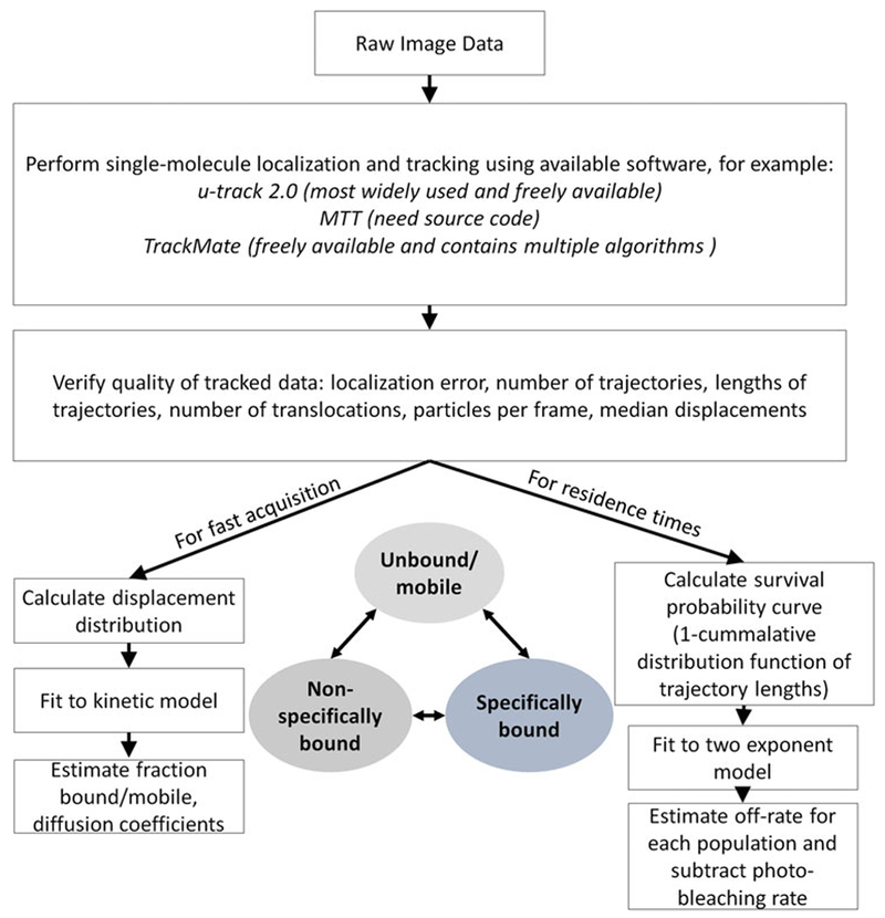
Summary of key steps for data analysis. Inset shows an example of a three-state model; the population in each state and the transition rates between states can be estimated from a combination of the fast and slow acquisition and data analysis
3.6. Single Molecule Imaging in Mice Embryos
The general guidelines for imaging in Drosophila embryos can also be used for imaging in blastocyst stage mice embryos (Fig. 5).
Mice embryos from a line with either a fluorescent protein or a HaloTag on the protein of interest should be collected. If using Halo-tagged protein, label the embryo with your organic dye of choice, and perform washing steps before mounting the sample on the LLSM.
Embryos can be mounted on a coverslip and immobilized using matrigel at high concentration.
Imaging condition optimization and data analysis should be performed as described above. See Fig. 5 for an example of single molecule imaging of JF549-labeled Halo-CTCF in an E4.5 late blastocyst mouse embryo.
Fig. 5.

Single molecule imaging in a mouse embryo. From left to right: (1) Bright-field image of an E4.5 late blastocyst mouse embryo chimera of wild type and JM8.N4 mES cells expressing endogenously tagged Halo-CTCF labeled with JF549. (2) Lattice light-sheet 3D image of the same embryo; red line indicates the lattice slice used for time lapse imaging of a single nucleus. (3) Single molecules of CTCF visible in a z-stack of a single nucleus in the same embryo. (4) Frame from 10 ms time series acquisition shown a single CTCF-binding event and corresponding PSF
Acknowledgments
The authors thank the Betzig lab at HHMI Janelia Research Campus for designs and advice on setting up the LLSM. We thank all members of the Darzacq, Tjian, Garcia, and Eisen labs for reagents, suggestions, and useful discussions. This work was supported by the California Institute of Regenerative Medicine (CIRM) LA1–08013 and the National Institutes of Health (NIH) UO1-EB021236 & U54-DK107980 to X.D., by the Burroughs Wellcome Fund Career Award at the Scientific Interface, the Sloan Research Foundation, the Human Frontiers Science Program, the Searle Scholars Program, and the Shurl and Kay Curci Foundation to H.G., a Howard Hughes Medical Institute investigator award to M.E., NSF Graduate Research Fellowships A.R. D.H. is a Pew-Stewart Scholar for Cancer Research supported by the Pew Charitable Trusts, the Alexander and Margaret Stewart Trust, the Siebel Stem Cell Institute, and NIH R01-CA196884.
4 Notes
The density of beads on the slide should be such that an isolated bead can be found for alignment easily.
The strength of the adhesive can be varied to your preference by increasing or decreasing the amount of scotch tape used.
If working with a fly line that is not laying well, the lids can be exchanged several times a day along with careful observation to determine the best time of the day for embryo collection.
If this is the first exchange after an overnight lay, it is good practice to perform a 90 min “clearing” lay before exchanging the lid again for your experiment. This helps reduce the occurrence of older than expected embryos in your experimental collection.
It is not necessary to have the objective water-heater blocks mounted for Drosophila experiments since they can be conducted at room temperature. Removing the blocks allows for using an appropriately positioned small LED lamp (e.g., Ikea Jansjo desk lamp) to provide bright-field-like images for quickly navigating the sample coverslip.
If using more than one fluorophore at a time, it is highly recommended to use a two camera setup with a separate set of filters and appropriate dichroic in between instead of recording the two colors sequentially on the same camera. Although the multicolor scanning in LLSM is sequential, commonly used fluorophores often have overlapping excitation or emission spectra or long tails, which can result in bleed through when using less than ideal filters such as multiband-pass emission filters.
We highly recommended using EMCCD cameras for single molecule imaging experiments at this point due to their higher quantum efficiency than most sCMOS cameras. Although the newest generation of sCMOS cameras has reported efficiencies that could be suitable for single molecule detection, we have not personally tested them.
Designing the correct lattice for your experiment should be done empirically. We have found that using a 30 beam pattern with a maximum numerical aperture 0.6 and minimum numerical aperture of 0.505 is suitable for single molecule imaging in fly embryos. Making the annulus thinner will result in more Bessel-like behavior (more side lobes but longer field of view) and conversely making it thicker results in more Gaussian-like illumination.
If using the LLSM design as originally described, it is recommended to use two Watt lasers as it will allow for uniform illumination while having sufficient power at the sample for single molecule imaging. If sufficient power cannot be achieved or if you only have lower power lasers, it is possible to adjust the laser collimation lenses to focus more of the energy in the center of the illumination pattern at the expense of the field of view over which the illumination is uniform.
It is very useful to have a vacuum trap connected to the main drain of the sample chamber to facilitate washing and rinse steps. If your system is not configured in this manner, it is worth to modify it to have this capability as it requires negligible effort, cost, and space.
Make sure to use the same medium for imaging and for alignment (e.g., for making up the dye solution for alignment). Small changes in salt concentrations result in large enough changes to the refractive index to cause misalignment.
It is useful and efficient to keep a reserved sample holder with a bead alignment slide loaded in for quick exchange during experiments for checking on suspected microscope drift.
5 mm coverslips can be cleaned in a petri dish by rinsing with clean deionized water, followed by sonication while immersed in isopropyl alcohol. Cleaned slides can be stored in isopropyl alcohol or dried and kept in a clean padded container.
Kimwipes can be cut into small 1 in. squares and stored in a tub. This smaller size is useful for wicking up and drying small areas and also reduces waste.
It takes 5–10 min for the glue to dry. It is prudent to check this by using your manipulation paintbrush prior to mounting embryos.
Many users may prefer to collect the embryos by hand using an inoculation loop or paintbrush instead of washing them out.
Timing the de-chorionation down to second precisely is not necessary. Embryos can also be de-chorionated manually by laying down a stripe of double-sided scotch top on a flat surface and gently rolling the embryos across it. Of course, this is much more labor and time intensive than using bleach.
Embryos that are not damaged or “punctured” will float to the top increasing the probability that only viable developing embryos are mounted on the coverslip.
As it can be difficult to manipulate the embryos once they are on the adhesive surface of the coverslip without damaging, an alternative method is to make an array of embryos on a pad of agar and then transfer them via gentle contact to the adhesive surface of the coverslip.
To set up a dedicated transillumination source for bright-field like imaging, install a LED source (e.g., Thorlabs MWWHL4) at the same angle as the detection objective just prior to the final flip mirror before the excitation objective. Using a lens the light from the LED should be brought to a focus in the back focal plane of the objective to have collimated light exiting the detection objective. With such a setup, it is possible to flip between the light sheet and transillumination by just flipping the final mirror.
We find this method of finding and marking all the embryos first more efficient as you don’t have to switch between bright-field and light-sheet illumination, but if you prefer you can check each embryo with LLSM imaging as you find them.
For example, for H2B-RFP with a 30 beam lattice, we typically need 0.5 mW of 561 nm illumination at the back aperture of the excitation objective at 50 ms exposure times.
To understand how to set the exposure time to access different timescales, you can think of the population of single molecules you are imaging to exist in three states: diffusing and thus moving quickly (typical D ~2–10 μm2/s), non-specific binding (short interactions; D < 0.1 μm2/s), and specific binding (long interactions; D < 0.1 μm2/s). Thus when measuring binding interactions, you can increase the exposure time (decrease the frame rate) such that diffusive mobile population motion blurs into the background, and you only get good signal from molecules that are bound or immobile for at least the length of the exposure. To access the diffusive population as well, you need to minimize the exposure time. Decreasing the exposure time naturally requires higher laser powers to achieve a suitable signal-to-noise ratio. Increasing the laser power results in faster photo-bleaching and thus the long binding times are not quantifiable, since binding times can generally only be accurately measured if the unbinding rate is higher than the photo-bleaching rate.
The SNR you require should be determined by the localization accuracy you require for your particular application in addition to being sufficiently high to allow high-confidence localization of single molecules.
If you are using a photo-switchable or photo-convertible fluorophore, a brief flash (typically the length of 1 exposure time) with the activation laser (typically 405 nm) is sufficient to convert enough molecules for imaging. If acquiring lengthier movies, you may need to use scripting to flash the activation laser periodically. We are currently exploring options to have a constant low-level of activation which would be more desirable than intermittent activation. If using a regular fluorescent protein at high densities, you may need to wait to photo-bleach enough molecules before single molecule detections are possible.
The fast nature of the early nuclear division cycles makes these experiments challenging. With practice you will determine the best window between divisions where the nuclei are not moving where reliable single molecule data can be acquired. The histone single molecule controls you should perform will also provide you with the dynamic range of your measurements and inform you on when you are limited by photo-bleaching and nuclear motion or drift for slow tracking or residence-time measurements. For fast tracking your fluorescent label fused with a nuclear localization signal (NLS) should be used as a control. Of course the exact sets of controls that are necessary will depend on your particular experiments.
In our recent work on Bicoid dynamics [9], we used an implementation of the dynamic multiple-target tracing (MTT) [15] algorithm to perform localization and tracking. A number of software options exist for both localization and tracking, and as this list is constantly evolving, it is left to the reader to decide on the appropriate one for their application. The MTT algorithm implementation that we have used will be provided upon request, and a MATLAB-based GUI of this implementation is available for download here: https://doi.org/10.7554/eLife.22280.022.
The localization accuracy can be calculated in a variety of ways. One way is to convert the signal to photon counts and calculate the uncertainty in the determined position using standard formulas for PALM/STORM microscopy. Second you may perform tracking on a fixed sample, calculate a mean-squared displacement curve, and determine the localization error from the intercept of the curve. If you are using spot-on [13] for analysis, it will estimate the localization error based on the data you provide.
References
- 1.Izeddin I, Recamier V, Bosanac L, Cisse II, Boudarene L, Dugast-Darzacq C, Proux F, Benichou O, Voituriez R, Bensaude O, Dahan M, Darzacq X (2014) Single-molecule tracking in live cells reveals distinct target-search strategies of transcription factors in the nucleus. eLife 3:e02230 10.7554/eLife.02230 [DOI] [PMC free article] [PubMed] [Google Scholar]
- 2.Chen JJ, Zhang ZJ, Li L, Chen BC, Revyakin A, Hajj B, Legant W, Dahan M, Lionnet T, Betzig E, Tjian R, Liu Z (2014) Single-molecule dynamics of enhanceosome assembly in embryonic stem cells. Cell 156 (6):1274–1285. 10.1016/jcell.2014.01.062 [DOI] [PMC free article] [PubMed] [Google Scholar]
- 3.Morisaki T, Muller WG, Golob N, Mazza D, McNally JG (2014) Single-molecule analysis of transcription factor binding at transcription sites in live cells. Nat Commun 5:4456 10.1038/Ncomms5456 [DOI] [PMC free article] [PubMed] [Google Scholar]
- 4.Mazza D, Abernathy A, Golob N, Morisaki T, McNally JG (2012) A benchmark for chromatin binding measurements in live cells. Nucleic Acids Res 40(15):e119 10.1093/nar/gks701 [DOI] [PMC free article] [PubMed] [Google Scholar]
- 5.Hansen AS, Pustova I, Cattoglio C, Tjian R, Darzacq X (2017) CTCF and cohesin regulate chromatin loop stability with distinct dynamics. eLife 6:e25776 10.7554/eLife.25776 [DOI] [PMC free article] [PubMed] [Google Scholar]
- 6.Cho WK, Jayanth N, English BP, Inoue T, Andrews JO, Conway W, Grimm JB, Spille JH, Lavis LD, Lionnet T, Cisse II (2016) RNA polymerase II cluster dynamics predict mRNA output in living cells. eLife 5:e13617 10.7554/eLife.13617 [DOI] [PMC free article] [PubMed] [Google Scholar]
- 7.Cisse II, Izeddin I, Causse SZ, Boudarene L, Senecal A, Muresan L, Dugast-Darzacq C, Hajj B, Dahan M, Darzacq X (2013) Real-time dynamics of RNA polymerase II clustering in live human cells. Science 341 (6146):664–667. 10.1126/science.1239053 [DOI] [PubMed] [Google Scholar]
- 8.Chen BC, Legant WR, Wang K, Shao L, Milkie DE, Davidson MW, Janetopoulos C, Wu XFS, Hammer JA, Liu Z, English BP, Mimori-Kiyosue Y, Romero DP, Ritter AT, Lippincott-Schwartz J, Fritz-Laylin L, Mullins RD, Mitchell DM, Bembenek JN, Reymann AC, Bohme R, Grill SW, Wang JT, Seydoux G, Tulu US, Kiehart DP, Betzig E (2014) Lattice light-sheet microscopy: Imaging molecules to embryos at high spatiotemporal resolution. Science 346(6208):439–439. 10.1126/science.1257998 [DOI] [PMC free article] [PubMed] [Google Scholar]
- 9.Mir M, Reimer A, Haines JE, Li X- Y, Stadler M, Garcia H, Eisen MB, Darzacq X (2017) Dense Bicoid hubs accentuate binding along the morphogen gradient. Genes Dev 31 (17):1784–1794 [DOI] [PMC free article] [PubMed] [Google Scholar]
- 10.Katz ZB, Wells AL, Park HY, Wu B, Shenoy SM, Singer RH (2012) Beta-actin mRNA compartmentalization enhances focal adhesion stability and directs cell migration. Genes Dev 26 (17):1885–1890. 10.1101/gad.190413.112 [DOI] [PMC free article] [PubMed] [Google Scholar]
- 11.Lucas JS, Zhang YJ, Dudko OK, Murre C (2014) 3D trajectories adopted by coding and regulatory DNA elements: first-passage times for genomic interactions. Cell 158 (2):339–352. 10.1016/j.cell.2014.05.036 [DOI] [PMC free article] [PubMed] [Google Scholar]
- 12.Chenouard N, Smal I, de Chaumont F, Maska M, Sbalzarini IF, Gong YH, Cardinale J, Carthel C, Coraluppi S, Winter M, Cohen AR, Godinez WJ, Rohr K, Kalaidzidis Y, Liang L, Duncan J, Shen HY, Xu YK, Magnusson KEG, Jalden J, Blau HM, Paul-Gilloteaux P, Roudot P, Kervrann C, Waharte F, Tinevez JY, Shorte SL, Willemse J, Celler K, van Wezel GP, Dan HW, Tsai YS, de Solorzano CO, Olivo-Marin JC, Meijering E (2014) Objective comparison of particle tracking methods. Nat Methods 11(3):281–U247. 10.1038/nmeth.2808 [DOI] [PMC free article] [PubMed] [Google Scholar]
- 13.Hansen AS, Woringer M, Grimm JB, Lavis LD, Tjian R, Darzacq X (2017) Spot-On: robust model-based analysis of single-particle tracking experiments. bioRxiv. 10.1101/171983 [DOI] [PMC free article] [PubMed] [Google Scholar]
- 14.Persson F, Linden M, Unoson C, Elf J (2013) Extracting intracellular diffusive states and transition rates from single-molecule tracking data. Nat Methods 10(3):265–269. 10.1038/Nmeth.2367 [DOI] [PubMed] [Google Scholar]
- 15.Serge A, Bertaux N, Rigneault H, Marguet D (2008) Dynamic multiple-target tracing to probe spatiotemporal cartography of cell membranes. Nat Methods 5(8):687–694. 10.1038/nmeth.1233 [DOI] [PubMed] [Google Scholar]