Abstract
Food image segmentation plays a crucial role in image-based dietary assessment and management. Successful methods for object segmentation generally rely on a large amount of labeled data on the pixel level. However, such training data are not yet available for food images and expensive to obtain. In this paper, we describe a weakly supervised convolutional neural network (CNN) which only requires image level annotation. We propose a graph based segmentation method which uses the class activation maps trained on food datasets as a top-down saliency model. We evaluate the proposed method for both classification and segmentation tasks. We achieve competitive classification accuracy compared to the previously reported results.
Keywords: image segmentation, graph model, weakly supervised learning, dietary assessment
1. INTRODUCTION
Six of the ten leading causes of death in the United States, including cancer, diabetes, and heart disease, can be directly linked to diet. Measuring accurate dietary intake is considered to be an open research problem in the nutrition and health fields. We have developed a mobile food record (mFR) system, also known as the Technology Assisted Dietary Assessment (TADA) system [1, 2] to automatically determine the food types and energy consumed by a person using image analysis techniques [3]. The accurate estimate of energy and nutrients using food image analysis is mostly based on the correctly labeled food item and a sufficiently well-segmented region. Food labeling per se relies on the correctness of interest region detection, which makes food segmentation extremely crucial.
In recent years the concept of deep learning [4] has been gaining widespread attention. As convolutional neural network (CNN) [5] gradually becomes dominant in many computer vision related areas, various recognition and classification tasks have been improved from the previous state-of-art methods [5, 6, 7]. Existing CNN models take advantage of labeled data which are used to learn which features are effective in a task as opposed to manually designed features. However, for more structured prediction, such as semantic segmentation, obtaining the pixel-level training data or even labeled bounding boxes is extremely time-consuming and expensive. For example, fully the convolutional network [6] requires careful annotation of the segmentation mask. Fast/Faster RCNN [7, 8] uses labeled data in the form of bounding boxes. Such dependency on fully supervised training poses a major limitation on scalability with respect to the number of classes or tasks [9].
In the field of food image analysis, there is no publicly available segmentation ground-truth image dataset. The bounding box information provided in the UECFOOD256 dataset [10] is far from sufficient. Im2Calorie [11] uses several CNN models to analyze food intake, but the authors have not yet released their Food-201 dataset. Therefore, we would like to explore weakly supervised learning where only image-level labels indicating the presence or absence of objects are required.
Semantic image segmentation, i.e. assigning a semantic class label to each pixel of an image, is an important topic in computer vision. Collecting fully annotated training data poses a major bottleneck to improve the segmentation models, thus weakly supervised training methods were proposed to reduce the annotation effort. Previous work [12, 13] on weakly supervised learning show that the output from a classification network can not only predict labels but also estimate object locations. In [14], a new loss function is proposed that uses location, classes and boundary priors to improve a segmentation system. Pourian [15] used a spectral clustering approach that groups coarse segmented image parts into communities. A community-driven graph is then constructed that captures spatial and feature relationships between communities while a label graph captures correlations between image labels. Finally, mapping the image level labels to appropriate communities is formulated as a convex optimization problem. In [13], Class Activation Map (CAM) for CNNs with global average pooling (GAP) are described. This enables classification-trained CNNs to learn to localize visual objects without using any bounding box annotations.
In this paper, we describe a graph based segmentation method for food images that uses a weakly supervised saliency model as prior knowledge. The contribution of this work is two-fold. First, we improve the CAM as a top-down saliency model by introducing a new pooling technique. Second, we incorporate the CAM trained on food datasets in the Biased Normalized Cut (Biased Ncut) segmentation method [16]. The proposed method shows promising results using various testing datasets, and we believe it can also be used as an initial step before manual ground-truthing.
2. NETWORK ARCHITECTURE FOR WEAKLY SUPERVISED LEARNING
Our model uses the fully supervised network of [17], known as VGG-16, that consists of 13 convolutional layers and 3 fully connected layers. To adapt the VGG-16 architecture to weakly supervised learning, we introduce several modifications. First, we add a 1024-channel convolutional layer and remove the first fully connected layer in the VGG-16 network. Second, we replace the max pooling layer before the fully connected layers with our proposed Global Max-Average Pooling (GMAP) layer. Figure 1 illustrates the proposed network architecture. We design the GMAP layer as a cascade combination of a Global Max Pooling (GMP) layer and a Global Average Pooling (GAP) layer. Furthermore, we extend the capability of GMAP by allowing adaptive pooling kernels. Similar to the ROI pooling layer [8], the size of pooling kernel varies based on the desired output, so that the output can be connected to a fully connected layer regardless of the size of the input images to the network.
Fig. 1.
Network architecture for weakly supervised learning.
Global Max-Average Pooling.
As discussed in [13], the GAP layer outputs the spatial average of the feature map at the last convolutional layer. For example, if there are 1024 feature maps at the last convolutional layer, the GAP will generate a 1024 dimensional vector. We adopt the Class Activation Map [13], which is essentially a weighted sum of the feature maps of the last convolutional layer.
GMP and GAP has been successfully used in previous studies [14]. However, they both have their disadvantages. GMP tends to underestimate the regions of objects as the max pooling technique encourages the response from the single location of the highest activation. And GAP is more prone to overestimate object sizes, because it takes all the activations into account. To overcome these disadvantages in the context of semantic segmentation, we propose a new pooling technique, namely GMAP. The cascade structure of max and average pooling can be viewed as a generalized pooling layer of GAP and GMP,
| (1) |
where W × W is the dimension of a feature map, fαis the window function of size α, β represents the stride of the max pooling kernel, and N = ⌊(W −α)/β⌋2. From Equation 1, we can see that F becomes GAP if we let α = β = 1 and it becomes GMP if we let α = W. At this point, the proposed network as shown in Figure 1 takes 224 × 224 RGB images as input and generates a 1 × 1 × 1024 vector after the GMAP layer and finally outputs a 1 × 1 × N vector of confidence scores. N is the total number of classes.
Adaptive Kernel and multi-label classification.
Region of Interest (ROI) pooling was first introduced in [8], which is essentially a simplified version of Spatial Pyramid Pooling (SPP) layer [18]. The goal of the ROI pooling layer or SPP layer is to adapt the various size of ROIs in the region proposal based networks. To complete the design of GMAP layer, we adopt the idea of the adaptive kernel. In other words, α in Equation 1 can be a function of W. Besides, the proposed network can also be extended to multi-label classification using multi-scale sliding window training as introduced in [12]. However, applying the adaptive kernel and multi-label training is not the focus of this paper. As shown in Section 4, we assume that one image only contains a single category of object.
3. GRAPH BASED SEGMENTATION
With the class activation map (CAM), the challenge is to use the prior knowledge for segmentation. It seems intuitive to incorporate salient stimuli [19] or fine-grained region proposals [20] into a graph model for the segmentation task. In [19] both bottom-up salient stimuli and object-level shape prior were integrated into min cut/max flow optimization. Such energy minimization is initialized with saliency map which is computed through context analysis based on multi-scale superpixels. Object-level shape prior is then extracted combining saliency with object boundary information. In [20], Cheng et al. implemented an iterative GrabCut [21] method which replaces user inputs with thresholded saliency maps.
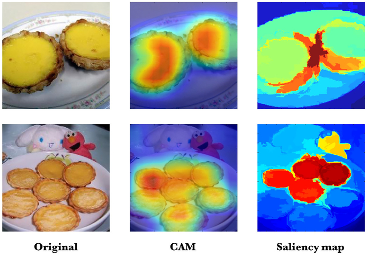
In this paper, we incorporate the sampled CAM as a top-down constraint in Biased Normalized Cut (Biased Ncut) [16]. Compared to a saliency map [19] as shown in Figure 2, the weakly trained CAM is better at localizing the object of interest. Given a region of interest in the image, i.e. the CAM in our case, we would like to segment the image so that the segment is biased towards the specified region. The image is modeled as a weighted undirected graph G = (V, E). The weight, w, on any edge, E, is a similarity measure between the end nodes of the edge. A region is modeled as a subset T ∈ V, of the vertices of the image. We are interested in the cut (, which not only minimizes the normalized cut value, N cut(S), but achieves sufficient correlation with the region specified by T, where
| (2) |
| (3) |
| (4) |
| (5) |
Fig. 2.
From left to right: the original image, its class activation map and saliency map [19].
Belief Propogation.
From Figure 2(b), we can see that the CAM peaks at where the network believes in showing the most prominent feature of a specific class in the image. However, it may not identify a part of the object as prominent even though the part of the object shares similar color and texture as its surroundings. To deal with this issue, we propose to use a multi-scale superpixel method to distribute the confidence that the network puts on certain regions in the image to their surroundings with similar color and texture.
Given an image, let [S1, …, Sp, …SP] be the superpixel mask at different scales, where P indicates the number of scales we use and let B be the initial CAM. For any pixel of a certain superpixel in Sp, we define its belief as follows,
| (6) |
where ||Sp|| represents the total number of pixels in the superpixel. So, if the superpixel is larger or the resolution of the superpixel mask is coarser, the belief is diffused more. We compensate the diffusal by introducing finer superpixel masks. Local variation [22] is used as the primary superpixel method because it is fast and relatively good at preserving edges. Finally, the new CAM is obtained by normalizing the original CAM and the propagated belief across all the superpixel scales,
| (7) |
where Z is a normalization term that makes sure B′(x, y) ∈ [0, 1].
Gassian Mixture Model and Sampling.
We use a Gaussian Mixture Model in the new CAM to generate a trimap [23]. A trimap normally partitions an image into three regions: a definite foreground, a definite background and an unknown region. Then the foreground is uniformly sampled with a fixed step, P, and these sampled points are used as seeds, sT, in the Biased Normalized Cut [16]. Given the graph G = (V, E), the Laplacian of G, LG and the normalized Laplacian, are defined as follows,
| (8) |
| (9) |
where DG and AG are the adjacency matrix and diagonal degree matrix of G. Finally, the optimal cut, x∗, is obtained by combining the eigenvectors of in the following way,
| (10) |
where λi represents the ith smallest eigenvalue, ui is the corresponding eigenvector and γ is a correlation parameter [16].
4. EXPERIMENTAL RESULTS
In this section, we describe our classification and segmentation experiments where we use several datasets to validate the proposed method, and we assume that one image only contains a single category of object.
Classification.
To validate the proposed pooling method, we trained various models using Caltech-256 [24], UECFOOD-256 [10] and Food-101 [25]. Caltech-256 [24] contains 30607 images of 256 object categories. UECFOOD-256 [10] consists of more than 31,000 images from 256 food categories, most of which are popular foods in Japan and other Asian countries. Food-101 [25] contains 101 food categories, each of which has 1000 images. Each dataset is randomly split in the 70/10/20 fashion for train/validation/test sets. We used a pretrained VGG-16 network to initialize the first 13 layers in our model and all the experiments were done in the Tensorflow [26].
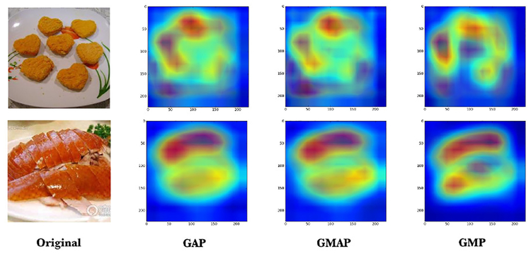
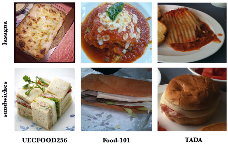
Table 1 compares the Top 1 classification acurracy of different pooling methods in the proposed network. Training the model with GAP was performed with stochastic gradient descent with learning rate of 0.01 and momentum of 0.9 while learning rate of 0.002 and momentum of 0.9 were used for the other pooling methods. GMAP – α – β represents GMAP with a α × α max pooling kernel and stride of β. As shown in the table, the network with GMAP −4−2 shows slightly better results across the three datasets. Figure 3 illustrates the visual differences of the CAMs when different pooling methods are used. Recently Yanai et al. reported 67.57% on the UECFOOD-256 using a modified AlexNet [27] and the best result, 78.11%, on the Food-101 is achieved using GoogleNet by Ao et al. [28]. Compared to their work, our model demonstrates comparable accuracy despite using a much simpler network architecture. Furthermore, we picked the images of 31 food categories from Food-101 [25] that are common in UECFOOD-256 and we named it the Food-31 dataset. We wanted to test the proposed model with GMAP − 4 − 2 trained on UECFOOD-256 [10] using the Food-31 dataset, since the images from these two datasets were initially collected from different sources and thus they should occupy slightly different domains in the feature space. As shown in Figure 4, the images of the same category look quite different in the different datasets. We achieved 85.8% accuracy over the 31,000 images in the Food-31 dataset without any fine-tuning.
Table 1.
Comparison of different pooling methods.
| Accuracy (%) | Caltech-256 | UECFOOD-256 | Food-101 |
|---|---|---|---|
| GMP | 81.05 | 63.97 | 72.75 |
| GAP | 81.09 | 64.01 | 72.78 |
| GMAP-2–2 | 81.20 | 64.80 | 73.81 |
| GMAP-3–3 | 81.05 | 64.01 | 73.55 |
| GMAP-4–2 | 81.53 | 64.89 | 74.02 |
Fig. 3.
Class activation maps using different pooling methods.
Fig. 4.
Examples from different datasets.
Segmentation.
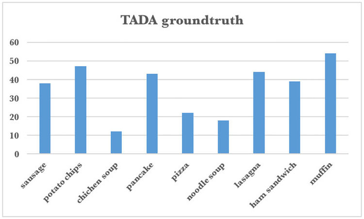
To evaluate the segmentation accuracy on the food images, we use a free-living study [29] from the TADA system. It consists of 1453 images of 56 commonly eaten food taken by 45 participants within a week, and we have manually ground-truthed over 900 food segments with labels. To our knowledge, there is no publicly available segmentation ground-truth for dataset food images yet and we would like to release our data for the academic use soon. Nine out of the 56 food categories in the free-living study have the same counterparts in the Food-101 [25] (see Figure 5) and there are 317 ground-truth in total.
Fig. 5.
TADA groundtruth statistics of 9 selected food categories which are common in the Food-101 dataset.
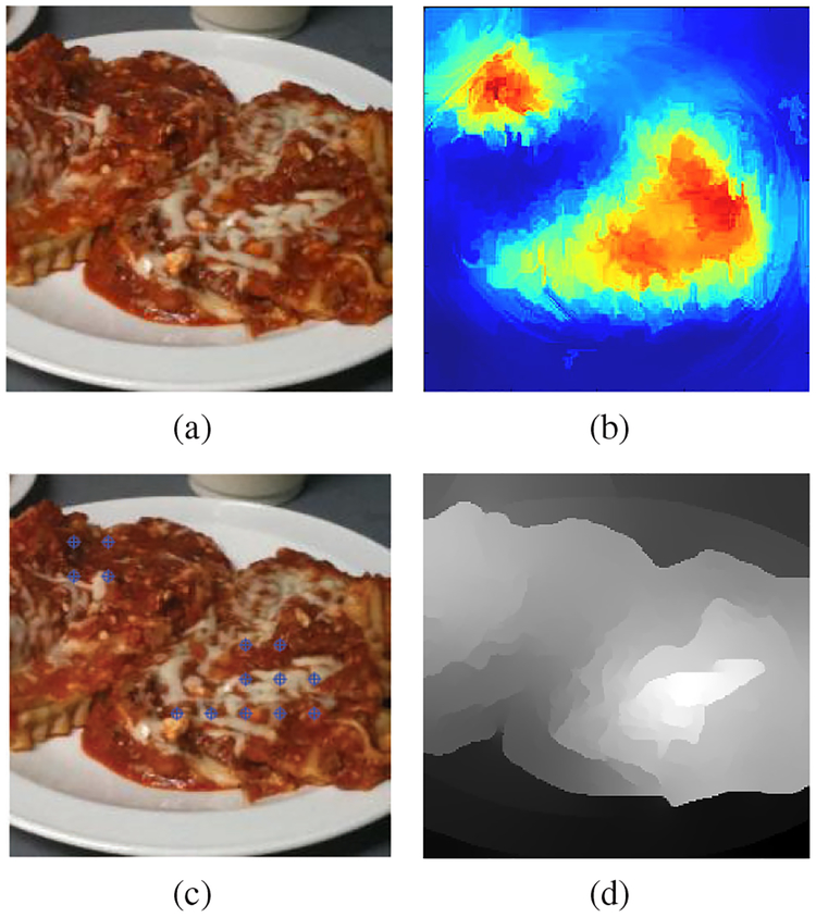
Based on our experiment, we choose P = 40, K = 16 and γ = 1e − 4 as discussed in Section 3. Figure 6 shows an example image from the free-living dataset. Seeds in Figure 6(c) are sampled from a trimap generated from Figure 6(b). Figure 6(d) represents the combination of the reshaped eigenvectors as discussed in Section 3.
Fig. 6.
(a) Original image. (b) The belief-propogated class activation map. (c) Seeds, sT as discussed in Section 3. (d) The biased normalized cut.
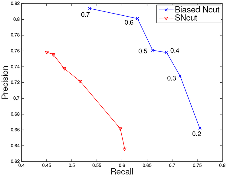
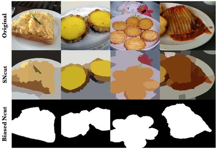
The final segmentation masks are obtained by binarizing the biased normalized cut. We use a region based metric [30] to evaluate the segmentation masks. Figure 7 shows the precision and recall [31] when various thresholds are used. Compared to our previous work, i.e. SNcut [32], the biased normalized cut based on the belief-propagated CAM demonstrates superior performance. More examples are shown in Figure 8.
Fig. 7.
Precision and recall of the segmentation results. Blue: Biased Ncut with the CAM prior. Red: SNcut
Fig. 8.
Example segmentation masks.
5. CONCLUSION AND FUTURE WORK
In this paper we described a weakly supervised CNN model with a new pooling technique and incorporate a class activation map for graph based segmentation. Our experiments shows promising results for both classification and segmentation tasks. In the future, we would like to test our model using a larger dataset and investigate multi-food segmentation.
Acknowledgments
This work was partially sponsored by the US National Institutes of Health under grant NIH/NCI 1U01CA130784–01 and NIH/NIDDK 1R01-DK073711–01A1, 2R56DK073711–04. Any opinions or recommendations expressed in this material are those of the author(s) and do not necessarily reflect the views of the US National Institutes of Health. Address all correspondence to Edward J. Delp, ace@ecn.purdue.edu or see www.tadaproject.org.
6. REFERENCES
- [1].Six BL, Schap TE, Zhu F, Mariappan A, Bosch M, Delp EJ,Ebert DS, Kerr DA, and Boushey CJ, “Evidence-based development of a mobile telephone food record,” Journal of the American Dietetic Association, vol. 110, no. 1, pp. 74–79, January 2010. [DOI] [PMC free article] [PubMed] [Google Scholar]
- [2].Zhu F, Bosch M, Woo I, Kim S, Boushey C, Ebert D, and Delp EJ, “The use of mobile devices in aiding dietary assessment and evaluation,” IEEE Journal of Selected Topics in Signal Processing, vol. 4, no. 4, pp. 756–766, August 2010. [DOI] [PMC free article] [PubMed] [Google Scholar]
- [3].Zhu F, Bosch M, Khanna N, Boushey C, and Delp E, “Multiple hypotheses image segmentation and classification with application to dietary assessment.” IEEE Journal of Biomedical and Health Informatics, vol. 19, no. 1, pp. 377–388, 2015. [DOI] [PMC free article] [PubMed] [Google Scholar]
- [4].LeCun Y, Bengio Y, and Hinton G, “Deep learning,” Nature, vol. 521, pp. 436–444, May 2015. [DOI] [PubMed] [Google Scholar]
- [5].Krizhevsky A, Sutskever I, and Hinton GE, “Imagenet classification with deep convolutional neural networks,” Proceedings of Advances in Neural Information Processing Systems, pp. 1097–1105, December 2012, Lake Tahoe, NV. [Google Scholar]
- [6].Long J, Shelhamer E, and Darrell T, “Fully convolutional networks for semantic segmentation,” Proceedings of the IEEE Conference on Computer Vision and Pattern Recognition, pp. 3431–3440, June 2015, Boston, MA. [DOI] [PubMed] [Google Scholar]
- [7].Ren S, He K, Girshick R, and Sun J, “Faster r-cnn: Towards real-time object detection with region proposal networks,” Proceedings of Advances in Neural Information Processing Systems, pp. 91–99, December 2015, Montreal, Canada. [Google Scholar]
- [8].Girshick R, “Fast r-cnn,” Proceedings of the IEEE International Conference on Computer Vision, pp. 1440–1448, December 2015, Santiago, Chile. [Google Scholar]
- [9].Pathak D, Krahenbuhl P, and Darrell T, “Constrained convolutional neural networks for weakly supervised segmentation,” Proceedings of the IEEE International Conference on Computer Vision, pp. 1796–1804, December 2015, Santiago, Chile. [Google Scholar]
- [10].Kawano Y and Yanai K, “Automatic expansion of a food image dataset leveraging existing categories with domain adaptation,” Proceedings of European Conference on Computer Vision Workshops, pp. 3–17, September 2014, Zurich, Switzerland. [Google Scholar]
- [11].Meyers A, Johnston N, Rathod V, Korattikara A, Gorban A, Sil-berman N, Guadarrama S, Papandreou G, Huang J, and Murphy KP, “Im2calories: Towards an automated mobile vision food diary,” Proceedings of the IEEE International Conference on Computer Vision, pp. 1233–1241, December 2015, Santiago, Chile. [Google Scholar]
- [12].Oquab M, Bottou L, Laptev I, and Sivic J, “Is object localization for free?-weakly-supervised learning with convolutional neural networks,” Proceedings of the IEEE Conference on Computer Vision and Pattern Recognition, pp. 685–694, June 2015, Boston, MA. [Google Scholar]
- [13].Zhou B, Khosla A, A. L, Oliva A, and Torralba A, “Learning Deep Features for Discriminative Localization,” Proceedings of the IEEE International Conference on Computer Vision and Pattern Recognition, June 2016, Las Vegas. [Google Scholar]
- [14].Kolesnikov A and Lampert CH, “Seed, expand and constrain: Three principles for weakly-supervised image segmentation,” Proceedings of European Conference on Computer Vision, pp. 695–711, October 2016, Amsterdam, Netherland. [Google Scholar]
- [15].Pourian N, Karthikeyan S, and Manjunath B, “Weakly supervised graph based semantic segmentation by learning communities of image-parts,” Proceedings of the IEEE International Conference on Computer Vision, pp. 1359–1367, December 2015, Santiago, Chile. [Google Scholar]
- [16].Maji S, Vishnoi NK, and Malik J, “Biased normalized cuts,” Proceedings of the IEEE International Conference on Computer Vision and Pattern Recognition, pp. 2057–2064, June 2011, Colorado Spring, CO. [Google Scholar]
- [17].Simonyan K and Zisserman A, “Very deep convolutional networks for large-scale image recognition,” CoRR, vol. abs/1409.1556, 2014. [Google Scholar]
- [18].He K, Zhang X, Ren S, and Sun J, “Spatial pyramid pooling in deep convolutional networks for visual recognition,” Proceedings of European Conference on Computer Vision, pp. 346–361, September 2014, zurich, Switzerland. [Google Scholar]
- [19].Jiang H, Wang J, Yuan Z, Liu T, Zheng N, and Li S, “Automatic salient object segmentation based on context and shape prior.” Proceedings of British Machine Vision Conference, vol. 6, no. 7, p. 9, September 2011, Nethergate, UK. [Google Scholar]
- [20].Cheng M-M, Mitra NJ, Huang X, Torr PH, and Hu S-M, “Global contrast based salient region detection,” IEEE Transactions on Pattern Analysis and Machine Intelligence, vol. 37, no. 3, pp. 569–582, 2015. [DOI] [PubMed] [Google Scholar]
- [21].Rother C, Kolmogorov V, and Blake A, “Grabcut: Interactive foreground extraction using iterated graph cuts,” ACM Transactions on Graphics, vol. 23, no. 3, pp. 309–314, 2004. [Google Scholar]
- [22].Felzenszwalb PF and Huttenlocher DP, “Efficient graph-based image segmentation,” International Journal of Computer Vision, vol. 59, no. 2, pp. 167–181, 2004. [Google Scholar]
- [23].Climaco JC and Antunes CH, “Implementation of a user-friendly software packagea guided tour of trimap,” Mathematical and Computer Modelling, vol. 12, no. 10–11, pp. 1299–1309, 1989. [Google Scholar]
- [24].Griffin G, Holub A, and Perona P, “Caltech-256 object category dataset,” California Institute of Technology, 2007. [Google Scholar]
- [25].Bossard L, Guillaumin M, and Van Gool L, “Food-101 – mining discriminative components with random forests,” Proceedings of European Conference on Computer Vision, vol. 8694, pp. 446–461, September 2014, zurich, Switzerland. [Google Scholar]
- [26].“TensorFlow: Large-scale machine learning on heterogeneous systems,” software available from tensorflow.org. [Online]. Available: http://tensorflow.org/
- [27].Yanai K and Kawano Y, “Food image recognition using deep convolutional network with pre-training and fine-tuning,” Proceedings of the IEEE International Conference on Multimedia & Expo Workshops, pp. 1–6, July 2015, Torino, Italy. [Google Scholar]
- [28].Ao S and Ling CX, “Adapting new categories for food recognition with deep representation,” Proceedings of the IEEE International Conference on Data Mining Workshop, pp. 1196–1203, November 2015, Atlantic City, NJ. [Google Scholar]
- [29].Schap T, Zhu F, Delp E, and Boushey C, “Merging dietary assessment with the adolescent lifestyle,” Journal of Human Nutrition and Dietetics, vol. 27, no. s1, pp. 82–88, 2014. [DOI] [PMC free article] [PubMed] [Google Scholar]
- [30].Malisiewicz T and Efros AA, “Improving spatial support for objects via multiple segmentations,” Proceedings of British Machine Vision Conference, September 2007, Coventry, UK. [Google Scholar]
- [31].Powers DM, “Evaluation: from precision, recall and f-measure to roc, informedness, markedness and correlation,” Journal of Machine Learning Technologyies, vol. 2, pp. 37–63, 2011. [Google Scholar]
- [32].Wang Y, Liu C, Zhu F, Boushey CJ, and Delp EJ, “Efficient super-pixel based segmentation for food image analysis,” Proceedings of the IEEE International Conference on Image Processing, pp. 2544–2548, September 2016, Pheonix, AZ. [DOI] [PMC free article] [PubMed] [Google Scholar]


