EFFICIENT SUPERPIXEL BASED SEGMENTATION FOR FOOD IMAGE ANALYSIS

Abstract

In this paper, we propose a segmentation method based on normalized cut and superpixels. The method relies on color and texture cues for fast computation and efficient use of memory. The method is used for food image segmentation as part of a mobile food record system we have developed for dietary assessment and management. The accurate estimate of nutrients relies on correctly labelled food items and sufficiently well-segmented regions. Our method achieves competitive results using the Berkeley Segmentation Dataset and outperforms some of the most popular techniques in a food image dataset.

1. INTRODUCTION

Six of the ten leading causes of death in the United States, including cancer, diabetes, and heart disease, can be directly linked to diet. Dietary intake, the process of determining what someone eats during the course of a day, provides valuable insights for mounting intervention programs for prevention of many of the above chronic diseases. Measuring accurate dietary intake is considered to be an open research problem in the nutrition and health fields. Our previous study [1] has shown the use of image based dietary assessment can improve the accuracy and reliability of estimating food and energy consumption. We have developed a mobile dietary assessment system, the Technology Assisted Dietary Assessment (TADA) system [2, 3] to automatically determine the food types and energy consumed by a user using image analysis techniques [4, 5].

The accurate estimate of energy and nutrients consumed using food image analysis is essentially dependent on the correctly labelled food item and a sufficiently well-segmented region. Food labeling largely relies on the correctness of interest region detection, which makes food segmentation extremely crucial. Although the human vision system is able to group pixels of an image into meaningful objects without knowing what objects are present, effective object segmentation from an image is in general a highly unconstrained problem [4].

Image segmentation is a process of partitioning an image into several disjoint and coherent regions in terms of some desired features. Segmentation methods can be generally classified into three major categories, i.e. region grouping methods [6, 7], contour to region methods [8, 9, 10], and graph-based methods [11, 12].

Alpert et. al [7] proposed a bottom-up probabilistic framework using multiple cue integration. It showed promising results when compared to other approaches. An example of a contour to region method is the hierarchical segmentation introduced in [9]. This has lead to several methods based the global probability of boundary (gPb), Ultrametric Contour Map (UCM) [9], and then methods that transform a contour into a hierarchy of regions while preserving contour quality [13]. Donoser et. al [10] proposed to locally predict oriented gradient signals by analyzing mid-level patches to reduce computational time of UCM. The common theme for graph-based approaches is the construction of a weighted graph where each vertex corresponds to a pixel or a region of the image. The weight of each edge connecting two pixels or two regions represents the likelihood that they belong to the same segment. A graph is partitioned into multiple components that minimize some cost functions. There are mainly two types of graph-based approaches: merging and splitting. The efficient graph based method, also known as local variation (LV) proposed by Pedro et al [11] is a merging method. It is an efficient algorithm in terms of computation complexity. Among splitting methods, normalized cuts (Ncut) [12] is extensively used.

Due to the complexity of food images (e.g. occlusion and cluttered background), food image segmentation is a difficult task. In[14], researchers experimented on 10 kinds of food with containers, thus formable part model and a circle detector were used to constrain the food region of interest. Bettadapura et. al [15] used hierarchical segmentation in their implementation. A semantic segmentation method based on deep neural network was recently proposed in [16]. Such method requires huge amount of manually segmented food images. [17] focuses on restaurant foods and utilize GPS information to get restaurant menus. With the correct restaurant information, they do not really need food segmentation, because they can already map the dish name to the responding nutrient table.

Food image segmentation has been extensively addressed in our previous work resulting in a joint segmentation/classification multiple hypothesis technique [4]. We also investigated the use of local variation and integrated it with food classifiers so that we can iteratively use the classification results to refine the segmented regions [5]. For each segment, a set of color, texture and local region features are used for our learning network, including the use of k-Nearest Neighbor (KNN), vocabulary tree and Support Vector Machine (SVM) [18].

In this paper, we propose a simple yet effective segmentation method that integrates normalized cut and superpixels using multiple features. This method is different than our previous work in that we do not use a feedback approach and we construct a new graph model. The main contributions are summarized as follows: (1) we introduce an efficient way of constructing weighted graph based on superpixels in multiple feature spaces, (2) we proposed a new image segmentation evaluation method which is specifically suitable for multi-food images, (3) we evaluate the proposed method on both the publicly available Berkeley Segmentation Database and our own food dataset. We are able to achieve competitive results, especially for food segmentation.

2. PROPOSED METHOD

General graph-based segmentation methods use low level features to measure similarity between two sets of pixels. For example, Ncut uses pixel intensity and difference of oriented Gaussian filter [12]. For an image of a complicated scene, using low level features often result in noisy segments. Another drawback with Ncut is the increase in computation associated with increased image size. “Superpixels” often are referred as local groups of pixels which have similar characteristics [19]. Superpixel methods have several useful properties such as they usually align well with object contours if the objects are not too blurry or the background is not too cluttered. They also enforce local smoothness because pixels belong to a superpixel are often from the same object.

To address the above disadvantages using Ncut, intuitively we might want to combine Ncut with superpixels. We can obtain higher level features from superpixels and reduce the size of the affinity matrix in Ncut. We shall call this approach ‘SNcut.’ We will discuss below the challenges of doing this including superpixel denoising, graph formation and food segmentation evaluation.

2.1. Superpixels and Denoising

We use simple linear iterative clustering (SLIC) [20] to provide an initial segmentation in SNcut. SLIC is a fast and memory efficient method that address local clusterings of pixels in 5D space consisting of L, a, b from the CIELAB color space and x, y pixel coordinates. It has shown good performance for several popular segmentation datasets [20]. When SLIC tries to preserve the shape or boundary of objects, there is a tradeoff between the similarity measure in the LAB color space and spatial distance between pixels, also regarded as proximity. This sometimes results in small segmented regions scattering around the “true segment”. We propose to use a Gaussian filter with a variance, σ, on the original image and use a median filter [21] with a fixed radius in pixel, r, following SLIC to merge the noisy segments. We then construct a weighted graph by using the proximity and similarity in color and texture features within the superpixel neighborhood, which will be discussed in Section 2.2.

2.2. Proximity, Color and Texture Cues

When constructing the weighed graph of superpixels we only allow adjacent superpixels to be connected which ensures a local Markov relationship [22]. We use average RGB pixel values and a customized local binary pattern (LBP) [23], discussed below, as the color and texture cues for the superpixels. The average RGB pixel value is obtained for all the pixels in the corresponding superpixel. LBP is a particular case of the Texture Spectrum model proposed in [24]. The customized LBP feature vector is created in the following manner: (1) Examine each pixel that has a 3 × 3 neighborhood in the superpixel with its 8 neighbors. If the center pixel value in L channel is greater than its neighbor, the output is 1, otherwise 0. Following a clockwise order, concatenate the binary results in an 8-dimensional vector, (3) By using the resulting vector as a binary number, we can convert it to a decimal number and then construct a histogram for each superpixel, (4) Finally, the histogram is sampled into 9 bins and normalized.

To translate the color and texture features into edge weights in our graph model, we first use χ² test [25] in texture space and L₂ distance in color space to obtain similarity measures. The χ² distance between two LBP vectors, g and h, associated with two superpixels, S_g, S_h is defined as:

$$D_{texture}={\chi }^2(g,h)=\frac{1}{2}\sum _i\frac{{(g(i)-h(i))}^2}{g(i)+h(i)}$$ (1)

L₂ measure in the RGB space is denoted as D_color. We then map the similarity measurement to a probability estimate:

$$P_{texture}=e^{-\frac{D_{texture}}{{\sigma }_{texture}}},P_{color}=e^{-\frac{D_{color}^2}{{\sigma }_{color}}}$$ (2)

Based on the experiments, we set σ_color to be 255 and σ_texture = βD_texture, where β ∈ [8, 12]. Finally, the edge weight is obtained,

$$\begin{gathered} w_{g,h}=\mathbf{I}(P_{color},P_{texure})\text{max}\{P_{color},P_{texture}\}+ \\ (1-\mathbf{I}(P_{color},P_{texture}))\text{min}\{P_{color},P_{texture}\} \end{gathered}$$ (3)

where I(·) represents the indicator function:

$$\mathbf{I}(P_{color},P_{texture})=\{\begin{array}{cc}1,& P_{color}>{ϵ}_1,Ptexture>{ϵ}_2\\ 0,& \text{otherwise}\end{array}$$ (4)

2.3. Object Based Segmentation Evaluation

Similarity between the automatic segmented image and a human annotated image (ground-truth) can be used to evaluate the performance of proposed method. Existing segmentation evaluation metrics include region differencing assessments [26, 27, 28] which count the degree of overlapping between segmented regions, boundary matching [29] and [30], Variation of Information (VoI) [31] and non-parametric tests such as Cohen Kappa [32] and normalized Probabilistic Rand Index (PRI) [33].

Precision and recall [29, 30] are widely used in boundary-based segmentation evaluations. However, some types of error, such as an under-segmented region that overlaps with two ground-truth segments with only a few missing boundary pixels in between, cannot be detected by boundary-based evaluation. We believe for food image segmentation a precise segment of each food is preferred over partially accurate boundaries. We adopt the region-based precision and recall proposed in [26] and adjust several criteria to focus on the objects of interest, or foods in our case.

Let S = {S₁, S₂, …, S_M} be a set of segments in an image generated by a segmentation method and G = {G₁, G₂, …, G_N} a set of ground-truth segments of all foreground objects in the same image, where S_i (i = 1, …, M) and G_j (j = 1, … N) represent the individual segment respectively. M is the total number of segments generated by the segmentation method and N is the total numbers of segments of the ground-truth.

The precision P for segment S_i and ground-truth G_j can be defined as $P(S_i,G_j)=\frac{\left|S_i\cap G_j\right|}{\left|S_i\right|}$, where |A| is the total number of pixels in A. Similarly, the recall R for S_i and G_j can be defined as $R(S_i,G_j)=\frac{\left|S_i\cap G_j\right|}{\left|G_j\right|}$. The F-measure, F [34] can then be estimated using precision and recall:

$$F(S_i,G_j)=\frac{1}{\alpha \frac{1}{P(S_i,G_j)}+(1-\alpha )\frac{1}{R(S_i,G_j)}}.$$ (5)

where α is the weight. We do not have a preference between precision and recall, hence we set α = 0.5.

Furthermore, we want to know which objects in the image are correctly segmented and how accurate are those segments. It is likely that M ≠ N, hence we want to match each foreground segment S_i to a G_j where S_i and G_j represent the same object in the image. In order to fairly match the segments, we introduce the overlap score (O) [27], $O(S_i,G_j)=\frac{\left|S_i\cap G_j\right|}{\left|S_i\cup G_j\right|}$. Unlike precision and re-call, the overlap score is low for both over-segmentation and under-segmentation, but only high when the segmentation is precise and accurate. The evaluation is then done as follows:

1. The background ground-truth segment G_B can be found as $G_B=1-\underset{j=1}{\overset{N}{\cup }}{G}_j$.

2. For each segment S_i in S, P (S_i, G_B) and P (S_i, G_j) with all the G_j in G are estimated. If P (S_i, G_B) is higher than all the P (S_i, G_j) for all G_j, we consider (S_i) as a background segment.

3. For each remaining S_i, O(S_i, G_j) is estimated with all the G_j in G, and (S_i, G_j) is considered as a matched pair if it has the highest overlap score.

4. Let I_j = {S_i: (S_i, G_j) is a matched pair, i ∈ [1, …, M]} and l(I_j) be the number of elements in I_j that matches G_j, the precision for this image can be estimated as:

   $$P=\frac{1}{M}\sum _{\underset{l(I_j)\ne 0}{j=1}}^M\frac{1}{l(I_j)}\sum _{S_i\in I_j}P(S_i,G_j)$$ (6)

   The Recall and Overlap score can be estimated in a similar way.

The above conveys our ideas of “good food image segmentation”:(1) Compared to the natural image segmentation criteria, we do not care much about the background extraction because some simple filters are able to eliminate over-segmented background [5]. Classifiers are often more effective in differentiating background from foods.(2) We favor a precise food segment and punish over-segmentation by averaging all suitable matches, because classifying many small segments are time-consuming and often generates unreliable results.

3. EXPERIMENTAL RESULTS

In this section, we evaluate the proposed image segmentation method on the TADA food segmentation dataset (TSDS) and the Berkeley Segmentation Dataset (BSDS) [35]. The TSDS contains 200 hand-segmented food images, which are collected from a larger dataset including a total of 1453 images of 56 commonly eaten food items acquired by 45 users in natural eating conditions. Each image contains 5 different food items and 3 utensil items on average. The BSDS consists of 500 natural images of diverse scene categories. Each image is manually segmented by 5 human subjects on average.

3.1. TADA Food Dataset

In the TSDS, we mainly compare the proposed segmentation method with local variation [11] and hierarchical segmentation [9] for two reasons. First, based on our previous work [4, 5], local variation outperforms other methods including Ncut, Mean Shift, active contours for the goal of food segmentation. Second, hierarchical segmentation is a popular method for general image segmentation, and has recently been adopted for food identification tasks [15]. For the proposed method discussed in Section 2, we use σ = 0.9, r = 12, β = 10. ϵ₁, ϵ₂ ∈ [0.6, 0.8] and the number of superpixels ranging from 120 to 200 for the following experiment.

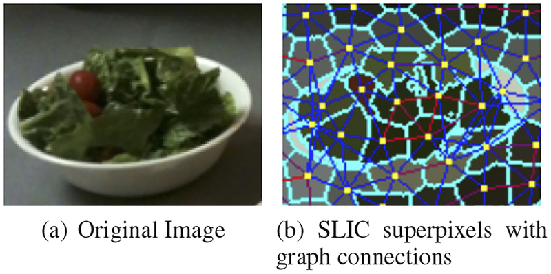
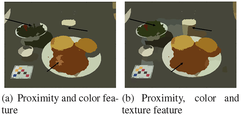
Figure 1 demonstrates the formation of the weighted graph using SLIC superpixels. In Figure 1, all the adjacent superpixels are connected based on their similarity in proximity, color and texture spaces. The red connections indicate that two superpixels are more similar while the blue connections show dissimilarity. Figure 2 shows the efficacy of the customized LBP feature. Using a graph model based only on color feature and proximity results in the image on the left. The image on the right takes texture feature into account as well. The black arrows in Figure 2 point at some of the segmentation variations. As shown in Figure 2(b), texture feature helps to include food regions with higher color variance.

Fig. 1.

SLIC superpixel with labeled graph connections. The red connections indicate two similar superpixels, and the blue connections indicate two dissimilar superpixels.

Fig. 2.

Proposed segmentation method with different features. Arrows points to areas of segmentation difference.

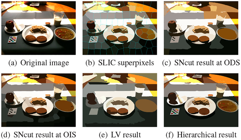
Figure 3 compares the results of SNcut to LV and hierarchical segmentation. We see that both SNcut and the hierarchical image segmentation are better at preserving the actual food contour thanLV. However, hierarchical segmentation is often sensitive to edges insides food items, resulting over-segmented regions, for example the noodle soup in Figure 3.

Fig. 3. Proposed segmentation method.

From (a) to (f): Original image, initial SLIC superpixels, SNcut output by thresholding at Optimal Dataset Scale [13], SNcut output by thresholding at Optimal Image Scale [13], output of LV and the hierachical segmentation (More examples are included in the supplemental material).

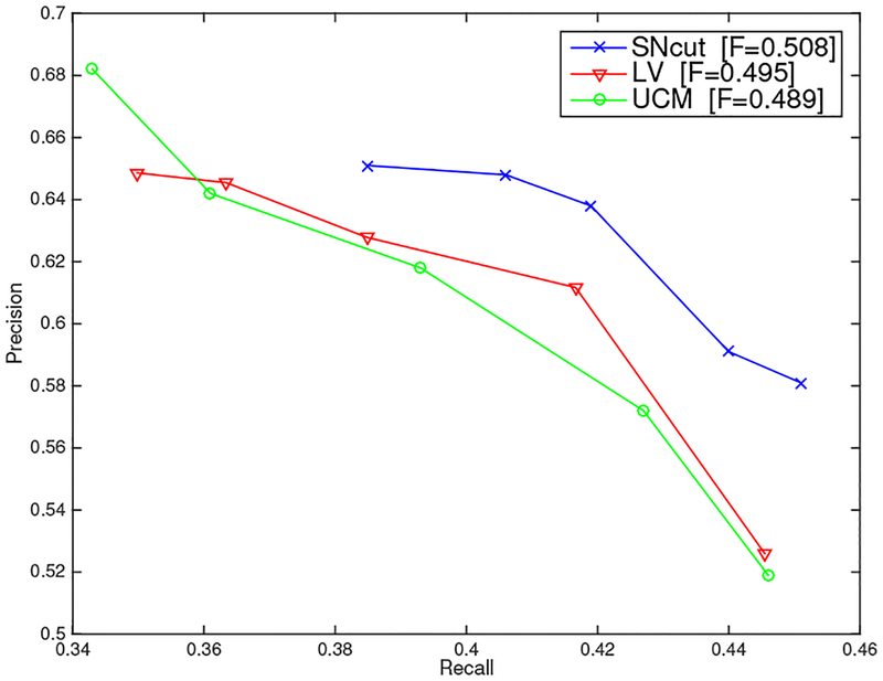
Figure 4 shows the PR curve and F-measure scores of SNcut, LV and hierarchical segmentation in different configurations. We evaluate all three methods using the object based evaluation metric discussed in Section 2.3. As illustrated, SNcut outperforms both LV and hierarchical segmentation. Due to the fact that our evaluation method averages precision and recall over the number of segments associated with a certain food ground-truth, both precision and recall scores are low when the image is severely under-segmented or over-segmented.

Fig. 4.

Precision and Recall on TSDS using the evaluation method discussed in Section 2.3.

3.2. Berkeley Dataset

We report 4 different segmentation metrics for the BSDS based on the region based evaluation method proposed in [13]: the Optimal Dataset Scale (ODS) or best F-measure on the dataset for a fixed scale, the Optimal Image Scale (OIS) or aggregate F-measure on the dataset for the best scale in each image, Variation of Information (VoI) and Probabilistic Rand Index (PRI). VoI computes the amount of information in ground-truth not contained in the segmentation result. PRI measures the likelihood of a pair of pixels being grouped in two segmentations. Better segmentation usually has higher PRI and lower VoI.

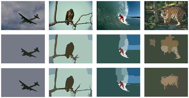
Some examples are shown in Figure 5. The scores are summarized in Table 1. The results for methods other than SNcut are collected from [13]. We see that SNcut improves the score from Ncut by a relatively large margin. However, SNcut does not obviously separate itself from other methods when it compares to the hierarchical segmentation or gPb-owt-UCM. gPb-owt-UCM trains on natural images to learn significant object contours, so it is more resistant to over-segmentation inside the object of interest when we set a proper threshold for the boundaries. Moreover, SNcut depends on the initial superpixel map to extract the objects of interest, which results in loss of global information. Compared with the objects in the natural images, foods usually have more homogeneous textures and more uniform colors. Thus, the way superpixels enforce local smoothness works better for food images.

Fig. 5. Proposed segmentation method.

From top to bottom: Original image, segmentations output by thresholding at ODS and OIS. We have included a supplementary file which contains more examples of our segmentation method.

Table 1.

Region based segmentation evaluation on the BSDS.

Methods	PRI	VoI	ODS	OIS
Ncut	0.75	2.18	0.44	0.53
LV	0.77	2.15	0.51	0.58
Mean Shift	0.78	1.83	0.54	0.58
SNcut	0.78	2.11	0.55	0.59
gPb-owt-UCM	0.81	1.68	0.58	0.64

On average, SNcut takes less than 3 seconds to segment one 481 × 321 image in BSDS. It is comparable to LV and 20 times faster than Ncut. For the full resolution 2048 × 1536 images in the TADA food dataset, SNcut takes 45 seconds to compute on average, which is 1.5 times faster than gPb-owt-ucm. All experiments were conducted on a desktop with quad core 3.7GHz CPU and 16GB RAM.

4. CONCLUSION AND FUTURE WORK

In this paper, we present a segmentation method that combines Ncut and superpixel techniques. We also introduce an object based segmentation evaluation method, especially for multi-food images. Experimental results suggest that the proposed method using multiple simple features is effective for food segmentation. According to our evaluation metric, SNcut outperforms some widely used segmentation methods and it also produces competitive results for natural images based on other segmentation benchmarks. In the future, we would like to investigate supervised learning on the weighted graph formation and explore a GPU implementation to further speed up the segmentation process.