Highlighting nerves and blood vessels for ultrasound-guided axillary nerve block procedures using neural networks

Abstract.

Ultrasound images acquired during axillary nerve block procedures can be difficult to interpret. Highlighting the important structures, such as nerves and blood vessels, may be useful for the training of inexperienced users. A deep convolutional neural network is used to identify the musculocutaneous, median, ulnar, and radial nerves, as well as the blood vessels in ultrasound images. A dataset of 49 subjects is collected and used for training and evaluation of the neural network. Several image augmentations, such as rotation, elastic deformation, shadows, and horizontal flipping, are tested. The neural network is evaluated using cross validation. The results showed that the blood vessels were the easiest to detect with a precision and recall above 0.8. Among the nerves, the median and ulnar nerves were the easiest to detect with an $F$-score of 0.73 and 0.62, respectively. The radial nerve was the hardest to detect with an $F$-score of 0.39. Image augmentations proved effective, increasing $F$-score by as much as 0.13. A Wilcoxon signed-rank test showed that the improvement from rotation, shadow, and elastic deformation augmentations were significant and the combination of all augmentations gave the best result. The results are promising; however, there is more work to be done, as the precision and recall are still too low. A larger dataset is most likely needed to improve accuracy, in combination with anatomical and temporal models.

1. Introduction

Ultrasound-guided axillary nerve blocks are used for local anesthesia of the arm as an alternative to general anesthesia. Ultrasound imaging is used to find the target nerves and the surrounding blood vessels. Local anesthetics are administered using a needle, which is usually visualized in the ultrasound image plane. The ultrasound images of these procedures can be difficult to interpret, especially for inexperienced users. Worm et al.¹ concluded in their study that ultrasound-guided regional anesthesia education focusing on still ultrasound images is not sufficient, whereas ultrasound videos and graphical enhancers may help students learn how to identify nerves in ultrasound. Wegener et al.² did an experiment with 35 novice subjects, who had performed $<30$ ultrasound-guided nerve blocks, on identification of nerves and related structures in ultrasound of several locations, including the axillary nerve block region. They observed that after a basic training course, one group of the participants failed to identify more than half of the anatomical structures while the other group, which received an additional tutorial, failed to identify one-third of the structures. These low identification scores of novices indicate that there is a need for better training tools.

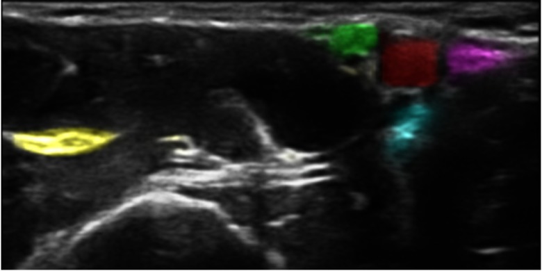
Image segmentation can be used to automatically identify the different critical structures in an image, such as nerves and blood vessels. Highlighting these structures in real time, as shown in Fig. 2, may be useful for training of inexperienced users. If good enough accuracy can be achieved, it may also be used for guidance during actual nerve block procedures.

Fig. 2.

The same image as in Fig. 1 is processed with the proposed method, which highlights the structures of interest. Even though the dataset is annotated with bounding boxes as shown in Fig. 1, the neural network performs segmentation, and each pixel’s estimated class is used to add color with a confidence-based transparency resulting in a highlighting effect.

Nerves are often difficult to distinguish from surrounding tissue in ultrasound images. In general, nerves appear as bright structures with black spots inside. Hadjerci et al.³ segmented the median nerve from ultrasound images using k-means clustering to find hyperechoic tissue, and then a texture analysis method based on a support vector machine classifier was used to identify the nerve. Hadjerci et al. developed this method further in Refs. 4 and 5. A segmentation method for the sciatic nerve in ultrasound images was presented by Hafiane et al.⁶ This method involved active contour segmentation driven by a phase-based probabilistic gradient vector flow. Smistad et al.⁷ created a guidance system for femoral nerve blocks, where the femoral artery and nerve were automatically segmented in real time. This system used a combination of the location of the artery, fascia, and presence of hyperechoic tissue to infer the location of the femoral nerve.

The short-axis cross section of blood vessels usually appears as dark ellipses in an ultrasound image. Several tracking methods based on using a Kalman filter have been proposed.^8–10 Most of these methods require manual initialization and are sensitive to user settings, such as gain on the ultrasound scanner.

In recent years, deep convolutional neural networks (CNNs) have achieved great results in image classification, segmentation, and object detection, even on challenging ultrasound images. There are some recent works using CNNs to find the nerves in ultrasound images. In 2017, Zhao and Sun,¹¹ and Baby and Jereesh¹² used a U-net CNN on the Kaggle dataset on ultrasound images of nerves in the neck. The appearance of nerves varies a lot depending on the patient and the location in the body. Creating a segmentation method that can accurately find nerves anywhere in the body is challenging. All previous studies, therefore, target specific nerves. CNNs have also been used to find blood vessels in ultrasound images. Smistad and Lovstakken¹³ used an image classification network to classify image patches of candidate vessel structures.

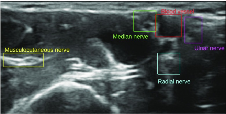
This paper investigates the use of CNNs to identify the four nerves (musculocutaneous, median, ulnar, and radial nerve) and blood vessels in ultrasound images acquired during axillary nerve block procedures. Figure 1 shows a typical example of an ultrasound image from this procedure. Compared to current state of the art, the presented method is able to identify and differentiate multiple nerves and blood vessels. Also, the method is validated on a relatively large dataset of 49 subjects with leave-one-subject-out cross validation. The end goal of this work is to highlight important structures in real time to aid in the training of clinicians and not to achieve a pixel perfect segmentation. The reason for distinguishing the four different nerves, instead of detecting all nerves as a single class, is to be able to highlight the different nerves with different color as shown in Fig. 2.

Fig. 1.

A typical example of an ultrasound image from the axillary nerve block procedure with the structures of interest annotated with bounding boxes.

2. Methods

2.1. Dataset

A dataset of 49 subjects was collected from both healthy volunteers and patients undergoing axillary nerve block procedures at St. Olavs Hospital in Trondheim, Norway. The study was approved by the local ethics committee and informed consent was given by all healthy volunteers. Informed consent was not required by the ethics committee for the patients, as these were routine acquisitions saved without any patient information. For each subject, one or more ultrasound videos were acquired, resulting in a total of 123 ultrasound videos. From each of these videos, one or more image frames were selected for annotation. The goal of selecting frames in a video was to capture frames that were as different as possible so that the final training set would cover as much variation as possible. Two annotated images that are almost identical contribute very little, if anything, to the training and can most likely be covered by image augmentations instead. Thus, if a video had almost no probe movement, only 1 image frame was selected from that video. More than one frame was selected if the probe was moved during the recording. The frames selected were then the ones that differed the most to the observer. In total, 462 image frames were extracted and manually annotated. All ultrasound recordings were acquired while the subjects were lying on their backs in supine position with the arm abducted 90 deg. The ultrasound probe was positioned on the arm, next to the arm pit, and perpendicular to the arm axis giving a short-axis view of the nerves, artery, and veins. Optimization of the ultrasound image is done by minor movements of the probe while keeping the artery in the image. Three different ultrasound scanners were used, Ultrasonix Sonix MDP (L14-5 transducer, 38 mm width, 6 MHz harmonic) (Analogic, Peabody), SonoSite M-Turbo, and SonoSite Edge (HFL38 transducer, 38 mm width, nerve application settings) (FUJIFILM SonoSite, Bothell). The imaging depth varied from 2.5 to 5 cm.

The location of each structure was annotated by an expert anesthesiologist using bounding boxes in an in-house web-based annotation tool. The reason for using bounding boxes instead of free-hand segmentation was to reduce the time needed to perform the annotation. Also, pixel-level accuracy was not required, as the goal was only to highlight the location of the structures.

After annotation, all images were resized to a width of 256 pixels while keeping the original aspect ratio. Images with a height above 256 pixels after resizing were cropped, and images with a lower height were padded with zero values so that the final image had a size of $256\times 256\text{pixels}$. An alternative would be to stretch smaller images. However, this would also stretch the blood vessels and nerves and might stretch the target structures to unnatural proportions.

2.2. Neural Network

Although the data were annotated using bounding boxes, a segmentation neural network was used. The reason for doing segmentation instead of bounding box detection was to achieve a confidence-based highlight visualization as shown in Fig. 2. Thus, the bounding box annotations described in Sec. 2.1 were converted into segmentation by setting all pixels in each box to the appropriate class.

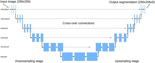
The fully convolutional U-net neural network architecture was used, as shown in Fig. 3. The U-net architecture consists of an encoder and decoder stage and has shown to work well on several medical image segmentation problems.¹⁴ The encoder performs several $3\times 3$ convolutions followed by $2\times 2$ max pooling in steps similar to an image classification network. The decoder stage performs upsampling and $3\times 3$ convolutions. The number of convolutions was doubled after each downsampling starting with eight convolutions on the first level and halved after each upsampling. Cross-over connections from the encoder to the decoder help to recover fine-grained image features from the encoder. The cross-over connections were concatenated with the upsampled features. Spatial dropout with a probability of 0.2 was used after each convolutional layer in the encoder stage.¹⁵ This dropout removes entire feature maps randomly and was essential for preventing overfitting on this dataset.

Fig. 3.

The U-net neural network architecture used in this work. For each level, two layers of $3\times 3$ convolutions were applied. In the encoder stage, every second convolution layer was followed by $2\times 2$ max pooling, and in the decoder, $2\times 2$ upsampling and concatenation with a cross-over connection.

The axillary nerve block segmentation problem in this paper has six different classes: (1) background, (2) blood vessel, (3) musculocutaneous (MSC) nerve, (4) median nerve, (5) ulnar nerve, and (6) radial nerve. Thus, the output layer of the neural network has six output channels for each pixel. A softmax activation function is used for the output. Each pixel is assumed to belong to exactly one class. The majority of the pixels will belong to the background class; thus, the Dice loss function is used for all classes except background. This loss function effectively avoids the class imbalance problem.

Training was performed using Tensorflow 1.8¹⁶ and Keras 2.0¹⁷ with the Adam optimizer,¹⁸ 50 epochs, and batch size 32.

2.3. Data Augmentation

The five following types of data augmentations were performed on the original dataset to increase the variability in the training data. The augmentations were generated on the fly using the original data while training. Since the parameter values of each augmentation are selected at random, this will in theory generate an infinite stream of distinct images. Nevertheless, the same original image was never used more than once in one epoch.

2.3.1. Horizontal flipping

Images were flipped horizontally with a probability of 0.5.

2.3.2. Rotation

Images were rotated with a random angle between $-10\mathrm{deg}$ and 10 deg.

2.3.3. Gamma intensity transformation

The image intensities were transformed with a random gamma value between 0.25 and 1.75 and clipped to a range between 0 and 1. This mimics the effect of using different settings for gain and dynamic range on the scanner.

$$I_g(x,y)=\min (1,\max (0,I{(x,y)}^{\gamma })).$$ (1)

2.3.4. Elastic deformation

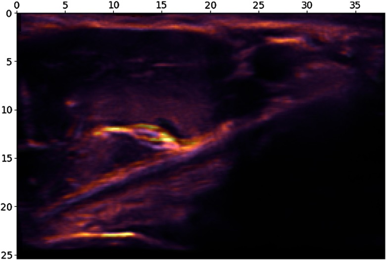
Elastic deformation was applied to the images using the approach of Simard et al.¹⁹ as shown in Fig. 4. The displacement fields are multiplied with a scaling factor of $\alpha$, which controls the amount of deformation. $\alpha$ was drawn from a uniform distribution of $[0.8,1.0]$ multiplied with the image width. The elasticity coefficient $\sigma$ was sampled from a uniform distribution of $[0.08,0.1]$ multiplied with the image width. The segmentation ground truth was transformed using the same deformation as the input image.

Fig. 4.

An example of elastic deformation. The original ultrasound image is superimposed on the deformed image. The scales are in millimeters.

2.3.5. Gaussian shadows

Ultrasound often has acoustic shadows due to air or tissue, which block acoustic energy from penetrating deeper in the tissue. To mimic this effect, a two-dimensional Gaussian shadow was randomly applied to the image in the following manner. A random pixel in the image was selected as the center for the shadow (${\mu }_x$ and ${\mu }_y$). The Gaussian’s standard deviations, ${\sigma }_x$ and ${\sigma }_y$, control the size of the shadow and were chosen from a uniform distribution between 0.1 and 0.9 of the image size. The strength of the shadow $s$ was drawn from a uniform distribution between 0.25 and 0.8. The Gaussian shadow image $G$ is then calculated as

$$G(x,y)=1-s{e}^{(-\frac{{(x-{\mu }_x)}^2}{2{\sigma }_x^2}-\frac{{(y-{\mu }_y)}^2}{2{\sigma }_y^2})}.$$ (2)

Finally, $G$ is pixelwise multiplied with the image $I$:

$$I_s(x,y)=I(x,y)*G(x,y).$$ (3)

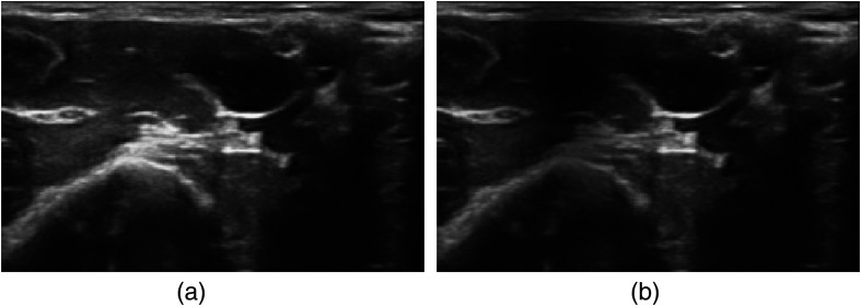
An example of a Gaussian shadow is shown in Fig. 5.

Fig. 5.

An example of a Gaussian shadow: (a) the original ultrasound image and (b) has an added Gaussian shadow.

2.4. Highlight Visualization

The highlight visualization shown in Fig. 2 was implemented in OpenGL using blending functions. The final color of a pixel $C_{\mathrm{F}}$ was calculated as the sum of the grayscale color of the ultrasound image $C_{\mathrm{US}}$ and the color $C_i$ of all $N$ structures multiplied by the confidence $c_i$ of class $i$ in the pixel:

$$C_{\mathrm{F}}=C_{\mathrm{US}}+\sum _{i=1}^N{C}_i{c}_i\alpha .$$ (4)

Thus, if the confidence is zero, no color is added to the ultrasound image, whereas for higher confidence, more color is added. A parameter $\alpha$ was used to scale the amount of coloring. Setting this value to 1 would give a complete coloring of areas with confidence 1, completely occluding the ultrasound image. Ideally, one would want to see both the ultrasound image and the structure’s colors, thus a value of $\alpha =0.3$ was used in this work. The authors believe this visualization is not only more visually pleasing than bounding boxes but also able to convey the neural network’s confidence on each pixel by scaling the coloring strength with the confidence.

2.5. Evaluation

Usually, image segmentation accuracy is reported using pixelwise metrics, such as Dice and Hausdorff distance. However, the goal of this work was only to highlight the nerves and blood vessels and not to have a perfect delineation of the structures. This also allows us to use simple bounding boxes for annotation, instead of free-hand segmentation, which is much more time consuming. Instead of pixelwise accuracy metrics, we calculate for each image whether the structures were found or not using the following criteria:

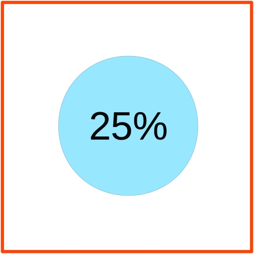
• •True positive: The structure was found. Twenty-five percent of the bounding box was classified as the correct structure (see Fig. 6).
• •False negative: A structure was not found. More than 75% of the bounding box was classified as the wrong structure.
• •False positive: An incorrect structure was found. Any segmentation region >$15\times 15\mathrm{pixels}$, $\sim 1.5{\mathrm{mm}}^2$, outside of an bounding box was considered a false positive.

Fig. 6.

At least 25% of a bounding box has to be classified as the correct class with a confidence above 0.5 to be counted as a true positive.

The reasons for using a limit of 25%/75% as shown in Fig. 6 for true positives and false negatives, respectively, are: (1) the bounding boxes are set to cover the entire structure, as most structures are not rectangular; this can leave a lot of background pixels inside the box. (2) Some bounding boxes are set larger than necessary when annotating. (3) The goal is not pixel perfect segmentation but only highlighting the location of the structures.

With these measures, recall and precision were calculated for each image. A confidence threshold has to be used to determine the class of a pixel. One option is to choose the class that has the highest confidence. However, in the worst case where each class has about the same confidence of $1/6=0.16$, a class with a confidence just above 0.16 would get selected, which is a very low value. On the other hand, a high threshold value of 0.9 would not leave much room for uncertainty. Thus, a confidence threshold of 0.5 was chosen.

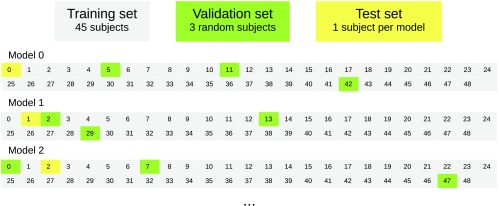
In machine learning, the dataset is usually divided into three sets: training, validation, and test set. To ensure an unbiased evaluation, leave-one-subject-out cross validation was used. Thus, a total of 49 neural network models were created, one for each subject. This is time consuming but gives a better impression of the expected results on data from a new subject. For each model, one subject was used as the test subject, three random other subjects were used for validation, and the rest for training as shown in Fig. 7. The best performing model on the validation data from all epochs was selected. All accuracy measurements were done per subject.

Fig. 7.

Leave-one-subject-out cross validation. Each number and square represent one subject.

3. Results

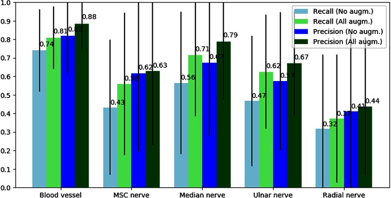
The average precision and recall of each structure for the cross validation are shown in Fig. 8. The precision and recall were calculated for each subject and then averaged for all the subjects. This was done for each of the five structures. The standard deviation was calculated to be in the range of 0.2 to 0.4 as shown in the figure. To see the effect of image augmentations, the results are presented with and without augmentations. Augmentations were only used during training.

Fig. 8.

Precision and recall per structure averaged over all subjects. The numbers above each bar are the average values and the black lines represent the standard deviation. The blue bars are the results with no augmentations, and the green results are with all the described augmentations.

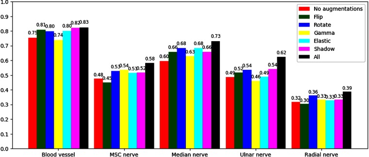
Figure 9 shows the effect of each augmentation method for each object. Here, the $F$-score, which combines recall and precision, was used to fit everything in one figure. A Wilcoxon signed-rank test was used to check for statistical significance in improvement in $F$-score compared to using no augmentations. The $p$-values for augmentations flip, rotate, gamma, shadow, and elastic were 0.335, $<0.001$, 0.583, $<0.001$, and 0.028, respectively. Thus, rotate, shadow, and elastic augmentations yielded a statistical significant improvement. The $p$-value of all augmentations combined was $<0.001$.

Fig. 9.

Comparison of the different augmentation methods using the average $F$-score.

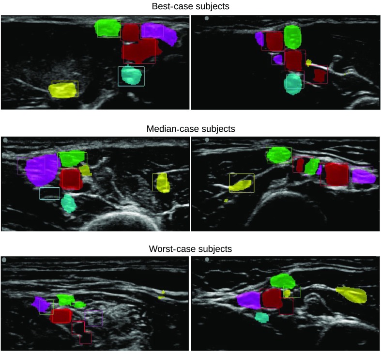
The $F$-score was also used to identify the best-, median-, and worst-case subjects. Two result images from each of these subjects are shown in Fig. 10. In these images, the bounding boxes of the expert annotations are shown in different colors for each structure. The highlight visualization was not used in this figure; instead, the pixels were given a fixed color if the confidence was above 0.5 for a given class. This was done to better show which pixels are actually used when calculating the accuracy.

Fig. 10.

Two result images from the best-, median-, and worst-case subjects in terms of $F$-score. The bounding boxes are the expert annotations, while the colored regions are the neural network output for each class thresholded at 0.5: blood vessels (red), MSC nerve (yellow), median nerve (green), ulnar nerve (magenta), and radial nerve (cyan).

Inference runtime of the network was within real-time constraints. The runtime was measured to be 10 ms on average for single frames using a NVIDIA Geforce GTX 1080 Ti GPU. Training took about half an hour per model.

A video showing the real-time highlighting on ultrasound recordings of the best, median, and worst cases in Fig. 10 has been uploaded and is available online.²⁰

4. Discussion

The results show that the CNN best detect the blood vessels with an average recall of 0.81 and precision of 0.88. This is not surprising as blood vessels are usually easily distinguishable from other types of tissue.

The MSC nerve is generally the most visible nerve as it is located inside a muscle. Muscles appear dark in ultrasound images, giving a good contrast to the hyperechoic nerve. Still, the results show that the neural network has more trouble finding the MSC nerve than the median nerve, which is more difficult to distinguish from surrounding tissue. This may be due to the fact that the median nerve is almost always located close to the axillary artery. By finding the artery, the CNN might more reliably guess where the median nerve is compared to the MSC nerve, which is usually located more distal to the artery.

The results also show that the radial nerve is the most difficult to detect. This is also the case for humans. The radial nerve is often located below the axillary artery and, therefore, not clearly visible at this position. However, this nerve can be easily visualized and blocked at the level of the elbow instead. One potential extension of this work would be to collect images from this area and annotate the radial nerve from this site as well.

The standard deviation for the precision and recall was high (0.25 to 0.4) for the nerves. Thus, the accuracy can vary a lot from one subject to the other, as shown in Fig. 10. This is most likely due to the high variation in anatomy and acquisition.

The comparison of different augmentation methods in Fig. 9 shows that each augmentation contributes to improved $F$-score, and the combination of all leads to the best overall $F$-score.

Direct comparison with previously published methods is difficult since we have not found any that target the axillary block and the four nerves present there. Previous work focuses on the median nerve at the forearm,^3–5 the sciatic nerve,⁶ the femoral nerve,⁷ or the brachial plexus of the neck (Kaggle competition).^11,12 Also, most of these studies use the pixelwise Dice score for evaluation, which is not directly comparable to the objectwise precision–recall detection scores. The reported Dice scores range from 0.65 to 0.9, whereas the Dice score in this work is lower than this because the dataset is annotated by bounding boxes while the neural network learns to perform segmentation. The most relevant work for comparison is the work of Hadjerci et al.⁵ from 2016, which performed automatic localization of the median nerve at the forearm. Their localization method achieved an average $F$-score of 0.70, which is comparable to the proposed method, which has an $F$-score of 0.73 for the median nerve at the armpit. However, the same nerve can appear differently when imaged at different places, such as the forearm and the armpit.

The main goal of this work was to create an application for training clinicians in interpreting ultrasound images for nerve block procedures. Whether the proposed system is accurate enough today for aiding training is hard to say and will require a follow-up study. One thing is certain: there is room for improving the detection results of the proposed highlighting method. In a training setting, where the volunteer to be scanned is known in advance, it is also possible to acquire one or two ultrasound images of this person in advance, have experts annotate the images, and run the training again. The neural network should then be able to learn the anatomical configuration of this person’s nerves and correctly highlight image planes different than the ones that were annotated while a novice user scans the volunteer.

More training data will most likely improve the accuracy by covering more anatomical and acquisition variations expected to be seen in the population. The fact that augmentations are increasing accuracy supports this belief, as augmentations create more training data, although with limited variation. Also, in a training setting, it should be possible to select subjects with average anatomy and good acoustic conditions.

Clinicians performing these kinds of procedures use real-time ultrasound to determine the position of the nerves. With real-time imaging, they can study the dynamics of the tissue by applying pressure with the probe and also see how the tissue moves with the pulsatile artery. The neural network in this paper only processes single images and, therefore, has no form of temporal memory. In addition to acquiring a bigger dataset, incorporating temporal information should be a key to improving the accuracy.

5. Conclusion

The results are promising in terms of real-time automatic highlighting nerves and blood vessels in peripheral nerve blocks. There is, however, more work to be done, as the precision and recall are still too low. Ultrasound images from axillary nerve block procedures exhibit large variation in anatomy and image quality, and the nerves can be hard to detect even for human experts in still images. A larger dataset is most likely needed to improve accuracy, in combination with methods that can incorporate anatomical and temporal information.

Biography

Biographies for the authors are not available.

Disclosures

No conflicts of interest, financial or otherwise, are declared by the authors.

References

- 1.Worm B. S., Krag M., Jensen K., “Ultrasound-guided nerve blocks—is documentation and education feasible using only text and pictures?” PLoS One 9(2), e86966 (2014). 10.1371/journal.pone.0086966 [DOI] [PMC free article] [PubMed] [Google Scholar]
- 2.Wegener J. T., et al. , “Value of an electronic tutorial for image interpretation in ultrasound-guided regional anesthesia,” Reg. Anesthesia Pain Med. 38(1), 44–49 (2013). 10.1097/AAP.0b013e31827910fb [DOI] [PubMed] [Google Scholar]
- 3.Hadjerci O., et al. , “Nerve detection in ultrasound images using median Gabor binary pattern,” in 11th Int. Conf. Image Analysis and Recognition 2014, pp. 132–140 (2014). [Google Scholar]
- 4.Hadjerci O., et al. , “Nerve localization by machine learning framework with new feature selection algorithm,” Lect. Notes Comput. Sci. 9279, 246–256 (2015). 10.1007/978-3-319-23231-7 [DOI] [Google Scholar]
- 5.Hadjerci O., et al. , “Computer-aided detection system for nerve identification using ultrasound images: a comparative study,” Inf. Med. Unlocked 3, 29–43 (2016). 10.1016/j.imu.2016.06.003 [DOI] [Google Scholar]
- 6.Hafiane A., Vieyres P., Delbos A., “Phase-based probabilistic active contour for nerve detection in ultrasound images for regional anesthesia,” Comput. Biol. Med. 52, 88–95 (2014). 10.1016/j.compbiomed.2014.06.001 [DOI] [PubMed] [Google Scholar]
- 7.Smistad E., et al. , “Automatic segmentation and probe guidance for real-time assistance of ultrasound-guided femoral nerve blocks,” Ultrasound Med. Biol. 43(1), 218–226 (2017). 10.1016/j.ultrasmedbio.2016.08.036 [DOI] [PubMed] [Google Scholar]
- 8.Abolmaesumi P., Sirouspour M., Salcudean S., “Real-time extraction of carotid artery contours from ultrasound images,” in Proc. 13th IEEE Symp. on Computer-Based Medical Systems, CBMS 2000, IEEE, pp. 181–186 (2000). 10.1109/CBMS.2000.856897 [DOI] [Google Scholar]
- 9.Guerrero J., et al. , “Real-time vessel segmentation and tracking for ultrasound imaging applications,” IEEE Trans. Med. Imaging 26(8), 1079–1090 (2007). 10.1109/TMI.2007.899180 [DOI] [PubMed] [Google Scholar]
- 10.Smistad E., Lindseth F., “Real-time automatic artery segmentation, reconstruction and registration for ultrasound-guided regional anaesthesia of the femoral nerve,” IEEE Trans. Med. Imaging 35, 752–761 (2016). 10.1109/TMI.2015.2494160 [DOI] [PubMed] [Google Scholar]
- 11.Zhao H., Sun N., “Improved U-net model for nerve segmentation,” Lect. Notes Comput. Sci. 10666, 496–504 (2017). 10.1007/978-3-319-71589-6 [DOI] [Google Scholar]
- 12.Baby M., Jereesh A. S., “Automatic nerve segmentation of ultrasound images,” in Proc. of the Int. Conf. on Electronics, Communication and Aerospace Technology, ICECA 2017, pp. 107–112 (2017). 10.1109/ICECA.2017.8203654 [DOI] [Google Scholar]
- 13.Smistad E., Lovstakken L., “Vessel detection in ultrasound images using deep convolutional neural networks,” Lect. Notes Comput. Sci. 10008, 30–38 (2016). 10.1007/978-3-319-46976-8 [DOI] [Google Scholar]
- 14.Ronneberger O., Fischer P., Brox T., “U-net: convolutional networks for biomedical image segmentation,” in Int. Conf. on Medical Image Computing and Computer-Assisted Intervention, pp. 234–241 (2015). [Google Scholar]
- 15.Tompson J., et al. , “Efficient object localization using convolutional networks,” in 2015 IEEE Conf. on Computer Vision and Pattern Recognition (CVPR), IEEE, pp. 648–656 (2015). 10.1109/CVPR.2015.7298664 [DOI] [Google Scholar]
- 16.TensorFlow , http://tensorflow.org (accessed 30 October 2018).
- 17.Keras , “Keras documentation,” http://keras.io (30 October 2018).
- 18.Kingma D. P., Ba J. L., “Adam: a method for stochastic optimization,” in Int. Conf. for Learning Representations (2015). [Google Scholar]
- 19.Simard P. Y., Steinkraus D., Platt J. C., “Best practices for convolutional neural networks applied to visual document analysis,” in Proc. Seventh Int. Conf. on Document Analysis and Recognition 2003, pp. 958–963 (2003). 10.1109/ICDAR.2003.1227801 [DOI] [Google Scholar]
- 20.Smistad E., “Video: Highlighting nerves and blood vessels for ultrasound axillary nerve blocks using neural networks,” YouTube, 4 November 2018, https://www.youtube.com/watch?v=06HTxmmu0mg. [DOI] [PMC free article] [PubMed]