Abstract
Accurate segmentation of infant brain images into different regions of interest is one of the most important fundamental steps in studying early brain development. In the isointense phase (approximately 6–8 months of age), white matter and gray matter exhibit similar levels of intensities in magnetic resonance (MR) images, due to the ongoing myelination and maturation. This results in extremely low tissue contrast and thus makes tissue segmentation very challenging. Existing methods for tissue segmentation in this isointense phase usually employ patch-based sparse labeling on single modality. To address the challenge, we propose a novel 3-D multimodal fully convolutional network (FCN) architecture for segmentation of isointense phase brain MR images. Specifically, we extend the conventional FCN architectures from 2-D to 3-D, and, rather than directly using FCN, we intuitively integrate coarse (naturally high-resolution) and dense (highly semantic) feature maps to better model tiny tissue regions, in addition, we further propose a transformation module to better connect the aggregating layers; we also propose a fusion module to better serve the fusion of feature maps. We compare the performance of our approach with several baseline and state-of-the-art methods on two sets of isointense phase brain images. The comparison results show that our proposed 3-D multimodal FCN model outperforms all previous methods by a large margin in terms of segmentation accuracy. In addition, the proposed framework also achieves faster segmentation results compared to all other methods. Our experiments further demonstrate that: 1) carefully integrating coarse and dense feature maps can considerably improve the segmentation performance; 2) batch normalization can speed up the convergence of the networks, especially when hierarchical feature aggregations occur; and 3) integrating multimodal information can further boost the segmentation performance.
Index Terms: 3-D fully convolutional network (3D-FCN), brain MR image, isointense phase, multimodality MR images, tissue segmentation
I. Introduction
The Increasing availability of noninvasive infant brain magnetic resonance (MR) images affords unprecedented opportunities for precise charting of dynamic early brain developmental trajectories in understanding normative and aberrant brain growth [1]. For example, the recently awarded Baby Connectome Project,1 will acquire and release cross-sectional and longitudinal multimodal MRI data from 500 typically developing children from birth to five years of age. This will greatly increase our limited knowledge on normal early brain development, and will also provide important insights into the origins and aberrant growth trajectories of neuro-developmental disorders, such as autism and schizophrenia. For instance, autistic children are reported to experience brain overgrowth associated with an increase in cortical surface area before two years of age [2]. As current treatments for many neuro-developmental disorders are ameliorative rather than curative, identifying early neuromarkers of risk for these disorders will allow designing targeted preemptive intervention strategies to improve prognosis or even prevent the disorders. To measure early brain development and identify biomarkers, accurate segmentation of MRI into different regions of interest (ROIs), e.g., white matter (WM), gray matter (GM), and cerebrospinal fluid (CSF), is the most critical step. It will allow for volumetric quantification and also more sophisticated quantification of the structures of GM and WM, such as cortical thickness, surface area, and gyrification, which may provide important indications of very early neuro-anatomical developmental events [3], [4].
The first year of life is the most dynamic phase of the postnatal human brain development. This is mainly because brain tissues grow rapidly, while cognitive and motor functions undergo a wide range of development [5]. Accurate tissue segmentation of infant brain MR images in this phase is of great importance in studying normal and abnormal early brain development [6]–[8]. It is recognized that the segmentation of infant brain MRI is considerably more difficult than the segmentation of adult brain MRI, due to reduced tissue contrast [9], increased noise, severe partial volume effect [10], and ongoing WM myelination [9], [11]. Fig. 1 shows examples of T1-weighted MRI, T2-weighted MRI, and fractional anisotropy (FA) image acquired at around six months of age. It can be observed that WM and GM exhibit almost the same intensity levels (especially in cortical regions), resulting in the lowest tissue contrast and hence significant difficulty for tissue segmentation.
Fig. 1.
Multimodality MRI data of an infant subject scanned at six months old (isointense phase). From left to right: T1 MRI, T2 MRI, and FA image.
Many methods introduced in [12] have been used for infant brain image segmentation. However, they mostly focused on the segmentation of either infantile images (≤ three months) or early adult-like images (>12 months) using a single T1 or T2 modality [13]–[18]. These images often demonstrate a relatively good contrast between WM and GM tissues. Few studies have addressed the difficulties of segmenting isointense-phase images. Shi et al. [19] first proposed a 4-D joint registration and segmentation framework for segmentation of infant MR images in the first year of life. In their method, longitudinal images in both infantile and early adulthood phases were used to guide the segmentation of images in the isointense phase. A similar strategy was later adopted in [20]. The major limitation of these methods is that they are entirely dependent on the availability of longitudinal datasets [21]. Considering that the majority of infant subjects comprise the data only from a single time-point, thus a standalone method working for cross-sectional single-time-point image is largely desired.
Recently, deep learning-based methods have achieved great success in image segmentation, including infant brain tissue segmentation. Zhang et al. [22] first proposed using deep convolutional neural networks (CNNs) to segment isointense-phase brain images, in which a hierarchy of increasingly complex features from MR images were learned. They used a patch-level learning by sliding windows in the 2-D space of the images. Their methods took the center voxel tissue label as the label for the whole patch during the learning. Consequently, their method was somehow sensitive to the patch size, especially for the voxels on the boundaries of WM or GM. In fact, such methods (based on the sliding windows) have to tradeoff between localization and classification accuracy, as utilizing large patches will lead to the loss in localization accuracy due to more pooling layers, while using small patches will yield perception of much less context information and thus become sensitive to noise. Moreover, these methods contain a large number of parameters, which over-burdens the convergence of the network. Moeskops et al. [23] further proposed a multiscale CNN for infantile brain tissue segmentation. Nie et al. [24] proposed a multipathway fully convolutional networks (FCN) to segment 2-D slices of infant brain tissue, while this model is very memory-costly due to the use of a multipathway architecture, and thus not suitable for 3-D MRI brain tissue segmentation. Chen et al. [25] introduced a residual learning technique to help the FCN training for the adult brain tissue segmentation. However, all the above-mentioned methods have overlooked the fact that CNN or FCN will lose information due to adoption of pooling operations, which will affect the localization accuracy.
To overcome the above-mentioned challenges, we propose to employ and further extend the FCNs [26] for the segmentation of infant brain image. FCN [26] is a special case of convolutional networks (ConvNets), in which the training is an end-to-end (pixel-to-pixel) process and embodies less network parameters. FCN consists of multiple convolution and pooling layers, which reduces the number of network parameters to a large extent, without incorporating any fully connected layers. Thus, FCN can simplify and speed up the processes of learning and inference in the networks, and make the learning problem much easier. FCN is able to take inputs of arbitrary size and generate same-size outputs, through efficient inference and learning. It generates dense pixel outputs by interpolating the coarse output via deconvolution layers. FCN has achieved state-of-the-art performance for semantic segmentation on multiple public datasets [26], [27] of 2-D images.
It is very important to note that the infant brain imaging data are in 3-D, and therefore a 3-D network structure should be developed and applied. Many recent works on medical images use the conventional 2-D architectures [22], [24], [28] or even utilize pretrained networks from natural images [26], [27]. In this paper, we propose a 3-D-FCN trained in an end-to-end and voxel-to-voxel fashion for segmentation of isointense-phase brain images. Our 3-D-FCN, similar to the conventional 2-D-FCNs, is composed of two major stages of convolution and deconvolution, each of which contains a number of layers to gradually down-sample or up-sample the image, respectively. Although FCN brings an improvement in segmentation, it still struggles in tiny structure tissue segmentation and precise localization, which are mainly due to the coarseness of feature maps and loss of resolution after series of pooling operations. Accordingly, to better model small structure tissues, we design an information pass-through (PT) architecture for our 3-D-FCN. Specifically, we utilize the coarse feature maps learned in the convolution process, which are of high-resolution and can be used to better localization. The deconvolution stage learns dense feature maps that are highly semantic and can help better classification, and we show that integrating them with the coarse feature maps, learned in the previous convolution layers, can help better segment tiny structure tissues. However, the number of neurons from coarse feature maps are usually much larger than that from dense feature maps, which could degrade the integration of the information by ignoring the signals from dense feature maps. We propose to use additional convolution operations to balance the biased signals problem. In addition, to effectively employ multimodality images, we feed MR images from different modalities into the designed neural network, through a batch normalization (BN) process. As explained later in more details, this intensifies better integration of multiple imaging modalities and also escalates the segmentation results, compared to the cases of using each modality separately or even only concatenating them through the same method. To implement the method on real images of isointense subjects, an input MR image is first partitioned into overlapping patches. For each patch, the trained model is used to predict a patch, corresponding to the label patch. Finally, all predicted label patches are merged into a single label image by averaging the label values in the overlapping regions. In summary, our contributions include the following.
We design a general 3-D FCN framework, which provides a tradeoff between resolution and abstraction by using less pooling operations and smaller convolution filters.
We further extend the initial model to aggregate coarse feature maps and dense feature maps. In addition, we propose a transformation module (e.g., 1 × 1 × 1 convolution layers) to balance signals from the aggregating layers; we also propose a fusion module (e.g., extra convolutional layers) to better serve the fusion of feature maps. These steps allow preserving the resolution in the final segmented image.
Furthermore, through the normalization procedure we incorporate, our architecture can integrate information from multiple modalities for the task of segmentation.
Our proposed method could achieve not only better segmentation precision but also much faster speed.
II. Method
Deep learning models can learn a hierarchy of features by building high-level features from low-level features. The CNNs (also known as ConvNets) [29]–[32] are one of the most popular types of deep learning models, in which the trainable filters and local neighborhood pooling operations are applied in an alternating sequence, starting with the raw input images. The convolution operation sequence can be described as (1) and (2), where l is the layer index (l=0, 1, … , n), al is the output of the lth layer (with a0 as the input data), and wl +1 and bl+1 are the weight and bias in the (l + 1)th layer which need to be learned, and f is the activation function. Equation (1) mainly describes the convolution procedure and (2) describes the nonlinear operation over the convolution result by activation function, such as rectified linear unit (ReLU) as described in (3). The last layer of CNNs is usually a softmax layer that is actually composed of cross entropy loss. The cross entropy loss can be formed as in (4). Note, in (4), m is the number of samples, k is the total number of tissue categories, x and y denotes data and label, respectively, θ is the parameter. The loss is back propagated to the whole network. When trained with appropriate regularization, CNNs can achieve superior performance on both visual object recognition and image classification tasks [22], [30], [32], [33]. Ji et al. [34] first proposed to use 3-D CNN to do human action recognition and achieved promising results
| (1) |
| (2) |
Where
| (3) |
| (4) |
Where
| (5) |
CNNs are also often used for image segmentation tasks. Besides, the FCNs [26], [27] have recently been proposed for image segmentation tasks as well. However, many of such methods use patch-based techniques for segmentation [35]–[37], thus depending heavily on the preprocessing or post-processing steps for patch extraction as well as post-refinement steps for the result enhancement. Our proposed technique trains in an end-to-end and voxel-to-voxel manner. On the other hand, the existing FCN often predicts dense outputs by feeding the whole image to the network and then learning through back-propagation. Upsampling layers are incorporated to enable voxelwise prediction. However, the traditional FCN have a big risk of losing resolution. To address this problem, we first design a basic FCN architecture which retains the resolution more by reducing times of pooling, and we further integrate features from lower layers into the higher layers to directly make up for resolution losses.
In the following, we will first introduce in Section II-A 3-D-FCN architecture (as shown in Fig. 2) by extending the conventional FCN [26] architecture to 3-D case, and then present the further extended 3-D-FCN model for multiple imaging modalities to more effectively use coarse and dense feature maps in Section II-B. Later, we give details of training in Sections II-C–II-E.
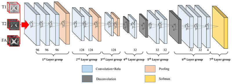
Fig. 2.
3-D-FCN architecture. Note, the number on the bottom row denotes the number of feature maps for the corresponding layers.
A. Designed Basic 3-D-FCN Architecture
One of the most challenging steps in adopting deep learning framework is the design of network architecture. The conventional FCN [26] utilize pooling operations four times which aims to highly abstracting the input information; however, the localization information could be seriously lost. We try to alleviate this problem by designing a basic framework to tradeoff the resolution and abstraction of input information. Inspired by Simonyan and Zisserman’s [32] work and Badrinarayanan et al.’s [38] work, we design our 3-D-architecture for MR images with groups of convolutional layers and de-convolutional layers, as shown in Fig. 2. Note, we only have utilized pooling operation three times, and use smallest convolution filters 3 × 3 × 3 which are believed to be able to capture the details better [32]. Reducing pooling operations will definitely mitigate the loss of resolution and we can have more layers with the small convolution filters which will keep the abstraction of information. This network applies softmax loss to the top layer of the networks. As demonstrated by Wang et al. [39] that the complementary information from multiple imaging modalities is beneficial to deal with insufficient tissue contrast, we thus feed three modality images as inputs to the neural network to learn complementary information from each other. In order to better use this complementary information, we further propose a PT architecture with BN procedure, as explained in detail in the following sections.
In our 3-D-FCN, the first group of layers consists of three convolutional layers (each containing 96 filters), followed by a pooling layer. These feature maps are fed into the second group of layers consisting of two convolution layers (each with 128 filters), followed by a pooling layer. In the third group of layers, one convolutional layer with 128 filters is applied, followed by a pooling layer. Note that all convolution filters are with a size of 3 × 3 × 3, and ReLU [40] is employed as an activation function after each convolution layer. We use one voxel as stride and add one voxel as pad for all convolution layers.
Then, the output feature maps from the third group of layers are up-sampled through a deconvolution layer to the fourth layer group with 32 filters. The fifth and sixth layer groups are both deconvolution layers with 32 filters, following the fourth layer group. The deconvolution filters are all of size of 4 × 4 × 4. In addition, the last deconvolution layer owns four filters, which correspond to four categories such as CSF, GM, WM, and background. It is worth noting that, similar to many previous works [26], [32], [38], we add convolution layers after each deconvolution operation. Finally, we have a top layer consisting of the softmax units, aiming at predicting one label (out of four possible labels) for each voxel.
Our network minimizes the cross entropy loss between the predicted labels and the ground-truth labels.
B. Convolution-Concatenate 3-D-FCN
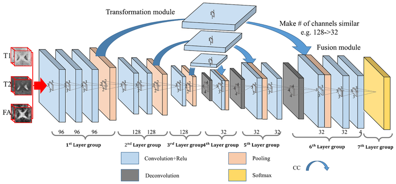
With the architecture introduced in the above section, FCN actually consists of two major operations: down-sampling and up-sampling. The down-sampling operation streams (i.e., convolution and pooling) usually result in coarse and global predictions based on the entire input of the network; and the up-sampling streams (i.e., deconvolution) can generate dense prediction through finer inference. The information which reaches up-sampling layers is highly abstracted after series of pooling operation, and thus can easily ignore tiny-structure objects, especially in the 3-D image. To solve this issue, we propose to include PT operations in our architecture, in which we take advantage of the context information from the coarse feature maps of the down-sampling set of operations and copy the whole learned feature maps to the up-sampling layers. This is similar to the operations used in [26], U-Net [28], and [41]. More importantly, we provide fusion modules (extra convolutional layers in our case) after the concatenation layers to enhance the fusion of the low-level and high-level features. In this way, we pass the context information from coarse feature maps through the network and use them in the up-sampling phases. This operation is thus called PT. As a consequence, the convolution layers during the up-sampling phase can generate more precise outputs based on the assembled feature maps. We call this architecture as PT-3-D-FCN.
However, the above described combination operation cannot well deal with the feature maps with different numbers (i.e., the original deeper layers usually have much less feature maps than the shallower layers), and thus the signals from the deeper layers can be ignored during the fusion operation. To address it, we propose using additional convolutional layers to adjust the number of feature maps from lower layers to be comparable to the number of the corresponding higher layers. Moreover, these additional convolutional layers can also work as transformation modules to boost the low-level features to be complementary for the high-level features. Note that this additional layer will not change the size of the feature maps, except adjusting just their numbers. The respective architecture is shown in Fig. 3, in which the whole PT operation is replaced by the convolution and concatenate (CC) subprocedures. We denote this model as CC-3-D-FCN for short. Furthermore, a BN [42] operation is adopted after each convolution operation to make the network easier to converge, as explained in more detail in the next section.
Fig. 3.
Proposed architecture for integration of coarse and dense feature maps (CC-3-D-FCN). Here, CC (blue arrow) denotes a convolution and concatenate subprocedure, which works as a transformation module. The convolutional layers after the concatenation layers work as fusion modules.
C. Batch Normalization
The training of 3-D deep learning architectures is always difficult, because it is much harder to converge compared to 2-D architectures [43], [44]. As we integrate lower-layer feature maps with high-layer ones, all these operations further increase the difficulty of network training because different layers have very different amplitudes [45]. And we have to account for this to aggregate the hierarchical feature maps. In this paper, we propose using BN [42] to solve this problem.
As the signals flow through our CC-3-D-FCN, the weights and parameters are applied to adjust these signals, which may sometimes make the signals too big or too small and may finally cause gradients vanishing or exploding. By normalizing the data in each mini-batch, this problem can be largely mitigated. Specifically, BN shifts the input signals to zero-mean and unit variance, and thus makes the data comparable across features. BN can regularize the signals from distraction to outliers and flow toward the common goal (by normalizing them), within the range of the mini-batch, which results in acceleration of the learning process.
D. Weight the Loss
In many real applications, like ours, the numbers of data samples from different categories are often different, and thus the distributions of the data between the sample classes are not balanced. This may cause over-fitting to a specific category, which is the so-called imbalanced data problem. To avoid this, we apply a class balance strategy during training. Specifically, we adopt a weighting scheme for the loss to address the class imbalance problem. The weighted cross entropy loss can also be formed as (4) but with (6) as the weight parameter (Cj is the loss weight for a specific category, and it can be given by inversely proportional to the fraction of samples in each corresponding category)
| (6) |
E. Training the 3-D-FCN
As it is the case with almost every medical imaging application, the dataset used to train a model is often limited, while almost all deep models require a huge number of samples for training [31], [44]. On the other hand, 3-D-FCN usually operates on full images as inputs in order to have broad receptive fields. To remedy these challenges and also to train a reliable deep model, we perform a tradeoff between receptive field and the dataset size. Specifically, we extract the overlapping patches of size 32 × 32 × 32 for both original images and manually segmented images. To augment the number of training patches, we slide the patch throughout the whole image with a certain step size. In this way, we can generate a sufficient number of training patches.
With the deep architecture shown in Fig. 3, the total number of parameters is 2 534 276. To train the designed network, we initialize its network weights using Xavier algorithm [44], which can automatically determine the scale of initialization based on the numbers of input and output neurons. We also initialize the network bias with 0. Then, we do a coarse linear search to determine the initial learning rate and also the weight decay parameters. We further decrease the learning rate by ten times for a fixed step size during training. The proposed model is trained by backpropagation [46]. Specially, we use Caffe [47], a commonly used deep learning framework, with minor modification to implement our proposed method.
III. Experimental Results
In this paper, we use data containing multimodality infant brain MR images to run the experiments and compare our proposed method with the baseline and state-of-the-art methods. We will first introduce the dataset and the respective preprocessing steps, followed by description of evaluation metrics.
A. Multimodality Infant Brain Dataset
For this dataset, we acquired T1, T2, and diffusion-weighted MR images of 11 healthy infants using a Siemens 3T head-only MR scanner. Both T2 image and the FA image (derived from distortion-corrected DWI) were first rigidly aligned with T1 image of the same infant and further up-sampled into an isotropic resolution of 1 × 1 × 1 mm3. T1 images were acquired with 144 sagittal slices using parameters: TR/TE = 1900/4.38 ms, flip angle = 7°, resolution 1 × 1 × 1 mm3. T2 images were acquired with 64 axial =slices using parameters: TR/TE = 7380/119 ms, flip angle 150° and resolution = 1.25 1.25 × 1.95 mm3. Diffusion-weighted MR images acquired with 60 axial slices using parameters: TR/TE = 7680/82 ms, resolution = 2 × 2 × 2 mm3, 42 noncollinear diffusion gradients, and =b = 1000 s/mm2; and seven nondiffusion-weighted reference scans were also acquired. We finally removed the skull, cerebellum and brain stem also from the aligned T2 and FA images with in-house tools. One example is shown in Fig. 1.
To generate manual segmentation for training, initial segmentation was first obtained with a publicly available infant brain segmentation software, iBEAT (http://www.nitrc.org/projects/ibeat) [48]. Then, manual editing was carefully performed by an experienced rater according to T1, T2, and FA images for correcting possible segmentation errors.
B. Evaluation Metrics and Comparison Methods
In the experiments, we focus on evaluating our proposed deep architectures for segmenting three types of infant brain tissues, and use Dice ratio as a performance metric
| (7) |
where A and B denote the binary segmentation labels generated manually and computationally, respectively, |A| denotes the number of positive elements in the binary segmentation A, and |A ∩ B| is the number of shared positive elements by A and B. We further evaluate the accuracy by measuring a modified Hausdorff distance (MHD) [49]. Supposing that C and D are the two sets of positive pixels identified manually and computationally, respectively, for one tissue class of a subject, the MHD can then be defined as
| (8) |
where d(C, D) =, (1/Nc) ∑c∈C d(c, D), and the distance between a point c and a set of points D is defined as d(c, D) = min ∑d∈D ‖c – d‖.
To show the superiority of our proposed method, we use the following methods as comparison methods in the experiments.
FMRIB’s Automated Segmentation Tool (FAST) [50].
Majority Voting (MV): For the 11-subject dataset, we employed a leave-one-strategy (for any testing image, the remaining ten subjects are used as atlases) and we used ANTs [51] for registration based on T1 MRI.
Random Forest (RF): In our implementation, for each tissue type, we randomly selected 10 000 training voxels for each class label from each training subject. Then, from the 7 × 7 × 7 patch of each training voxel, 10 000 random Haar-like features were extracted from all source images: T1, T2, FA images, and then we trained 20 classification trees. We stopped the tree growth at a certain depth (i.e., D = 50), with a minimum number of eight samples for each leaf node (smin = 8). Note that these settings have been optimized in LINKS [52].
RF With Auto-Context Model (LINKS) [52]: Based on the above-mentioned RF, we then apply the auto-context model to iteratively refine the results. Specifically, we not only extracted Haar-like features from all source images: T1, T2, and FA images, but also three probability maps of WM, GM, and CSF. And all the features were used to train the RF (note, it is now auto-context refined, and called LINKS). In each iteration, the training of model followed the RF settings introduced above.
Training CC-FCN for 2-D patches along each dimension, after which we perform MV for the results from different CC-FCN models (CC-2-D-FCN).
3-D-CNNs: The network shares the same three layer groups in Fig. 2, and followed by three fully connected layers, and the output corresponds to the center voxel of the input patch.
In the following sections, we will first discuss and evaluate the parameter selections as well as training strategies, and then present comparison with state-of-the-art methods.
C. Impact of Patch Size
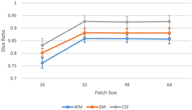
Patch size plays an important role in CNN-based methods, since it regulates the tradeoff between localization accuracy and the use of context [35]. However, FCN-based architectures can mitigate the impact of patch size on the segmentation tasks [24], [28]. To investigate the impact of patch size in this project, we conduct several experiments using four different input patch sizes: 16×16 × 16, 32 × 32 × 32, and 64 × 64 × 64 for training the same FCN architecture shown in Fig. 3. Fig. 4 shows the respective results (i.e., Dice ratio of segmentation as a function of patch size).
Fig. 4.
Changes of Dice ratios of WM, GM, and CSF on 11 isointense subjects, with respect to different patch sizes. Here, leave-one-subject-out cross validation is used.
As shown in Fig. 4, the segmentation performance is the worst with the patch size of 16 × 16 × 16, which provides the smallest context. With the patch size of 32 × 32 × 32, the segmentation task obtains the best performance. It is interesting to note that the Dice ratio becomes slightly worse when the patch size grows. This may be due to the fact that, when we use larger patch size, we will have smaller available number of patches to train the model, thus resulting in a lower performance. The result also shows that the FCN-based architecture is robust to patch size when the patch size is larger than a certain value. This advantage roots from the fact that the localization accuracy is stable when using FCN-based architectures. On the other hand, when the patch size is larger, the improvement may be limited by the number of extracted patches. With the insight gained through this experiment, we set the patch size to be 32 × 32 × 32 throughout all experiments below.
D. Importance of Multimodality Information
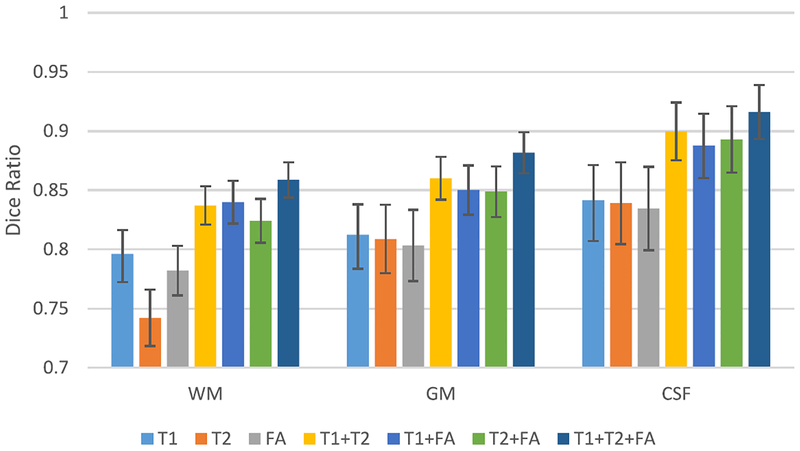
To demonstrate the effectiveness of using multimodality data (i.e., T1, T2, and FA in our experiments), we run the same model for each imaging modality separately, or together. Fig. 5 illustrates the Dice ratios of our proposed method with respect to different combinations of three imaging modalities. It can be seen that using more imaging modalities generally results in more accurate segmentations than using any single imaging modality. Moreover, using all three imaging modalities provides the best performance, compared to the cases of using any two imaging modalities. This indicates that the multimodality information is useful for guiding tissue segmentation. A same conclusion can also be drawn by looking into the experimental results on the second dataset as described below.
Fig. 5.
Average Dice ratios of our proposed method with respect to different combinations of three imaging modalities.
E. Importance of Using the Additional Convolution Before Concatenation
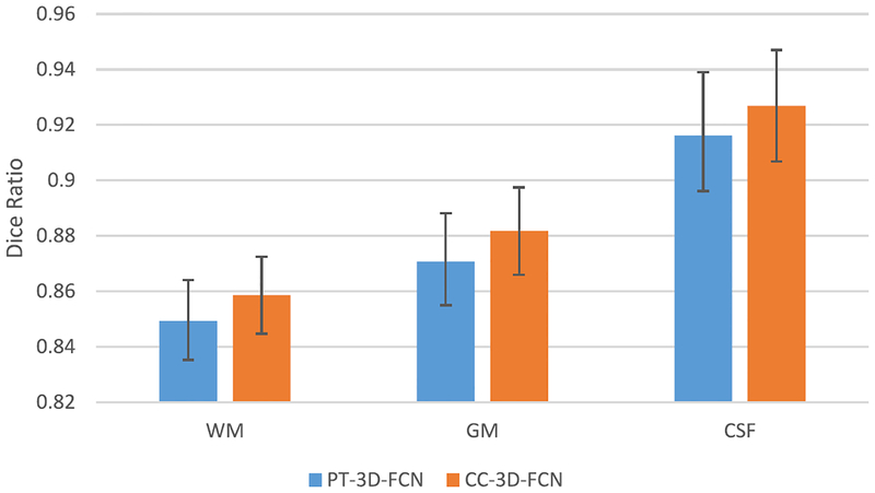
As described in Section II-B, we utilize an additional convolution layer on the coarse feature maps before concatenating them with dense feature maps. As discussed before, this layer is used to reduce the potential bias effect when directly copying the signals to the higher layer. We conduct some experiments to compare the networks with (CC-3-D-FCN) and without (PT-3-D-FCN) the additional convolution layer on the 11-subject dataset. All experimental settings are the same except using the additional convolution layer. The experimental results in terms of Dice ratio are shown in Fig. 6. As can be seen, CC-3-D-FCN outperforms PT-3-D-FCN on all three brain tissues, suggesting that the use of additional convolutional operations benefits the discrimination capability.
Fig. 6.
Comparison of CC-3-D-FCN and PT-3-D-FCN.
F. Importance of Batch Normalization
The proposed architecture (as shown in Figs. 2 and 3) involves information fusion from different modalities or sources. Information from different sources usually have different distributions, which could bring difficulty in training neural networks [44], [53]. Moreover, we combine hierarchical feature maps in our designed architecture, which further increases the difficulty of training. The use of BN [42] in our model plays a key role in solving this problem as explained below.
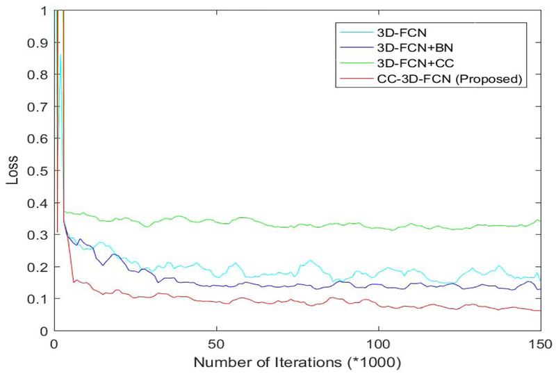
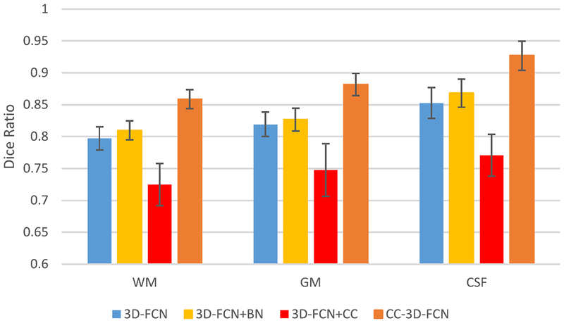
To show the advantage of using BN in our architecture, we present the loss on the testing dataset in Fig. 7. Also, we provide the performance in terms of Dice ratio with respect to different training strategies in Fig. 8.
Fig. 7.
Comparison of different training strategies in terms of loss on the testing dataset.
Fig. 8.
Average Dice ratios of our proposed method with different training strategies.
The loss values obtained during the training of network as shown in Fig. 7 indicates that 3-D-FCN + BN can decrease the loss a little bit. And our proposed method (combining 3-D-FCN, BN, and CC) provides the lowest test loss, which confirms that the CC operation along with the BN can help improve the performance of neural networks. In contrast, 3-D-FCN+CC gives the worst performance, which again shows that BN is critical in training networks. This is because when the data with different distributions and settings are incorporated from other layers, the BN operation can bring them into a same space before conducting the proceeding steps. The segmentation performance shown in Fig. 8 is consistent with our findings as discussed above for training the FCNs.
G. Impact of Network Initialization Strategies
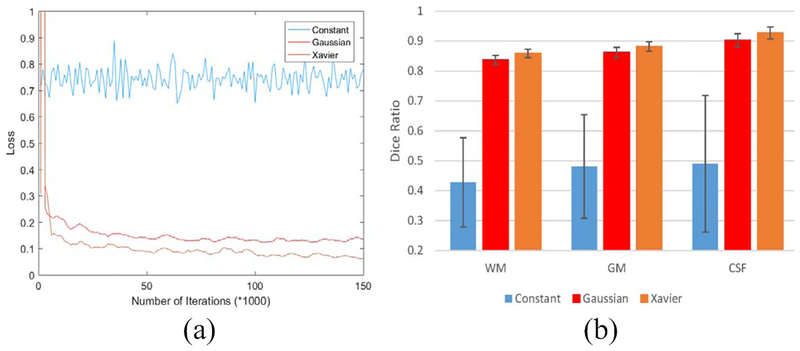
We further explore the impact of network initialization over the network training and the performance of the segmentation task. Specifically, we use the following strategies to initialize the network, respectively, i.e., constant (0), Gaussian (0, 0.01), and Xavier [44]. All other settings are kept the same, and we present the convergence with different initializations in Fig. 9. Obviously, the “constant” initialization cannot guarantee a converged training, while “Gaussian” and “Xavier” initializations can both result in good convergence. As it is obvious, using Xavier to initialize the network leads to the best performance.
Fig. 9.
Comparison of different initialization strategies in the proposed model. (a) Convergence situation. (b) Segmentation performance.
H. Impact of Pooling Layers: Pooling-Included Versus Pooling-Excluded Networks
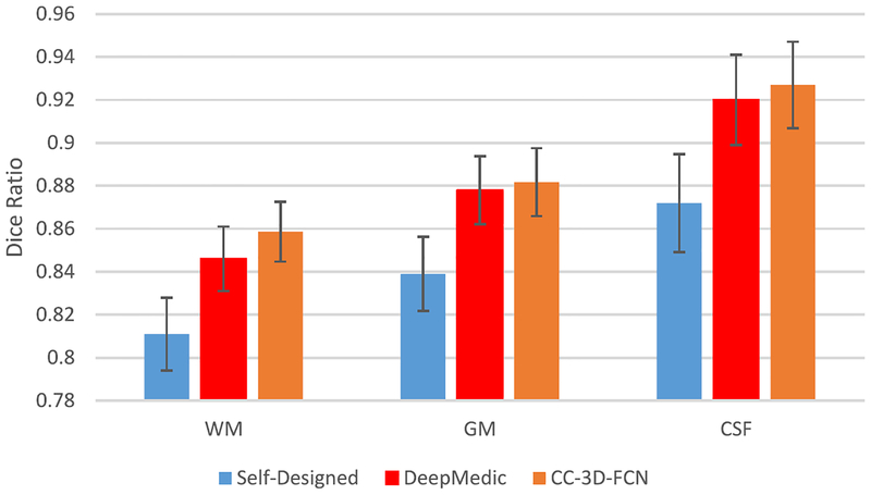
In the FCN-based network architectures (pooling-included network, e.g., our designed network), pooling is an important component to increase the receptive field dramatically and produce invariant feature representation. However, it will also result in the loss of spatial information. In our designed network (Fig. 3), we propose to use a skip connection to aggregate the shallower (high-resolution) layers and the deeper (highly semantic) layers, aiming at making up the lost information. Another possible way to avoid the loss of spatial information is to exclude the pooling layers and include only the convolutional layers (pooling-excluded network). To see the importance of pooling layers, we conducted comparisons between our designed network with pooling layers and two pooling-excluded networks.
Self-Designed: The network is with 11 convolutional layers, with each layer having 3 × 3 × 3 convolution filter (to satisfy the requirement of receptive field, as the input patch size is 32 × 32 × 32), but no pooling layer.
DeepMedic: The popular 3-D multiscale CNN (DeepMedic) [54], which was well-designed and showed excellent performance in lesion labeling.
The experimental results are presented in Fig. 10. The pooling-included network (our proposed model) works better than the other two pooling-excluded networks, indicating that the use of pooling-included networks with skip-connection is a better choice for our segmentation tasks. DeepMedic works better than the self-designed network, since multiscale designed network partially alleviates the insufficient receptive field problem and learns invariant features.
Fig. 10.
Comparison between pooling-included network and pooling-excluded networks (self-designed and DeepMedic).
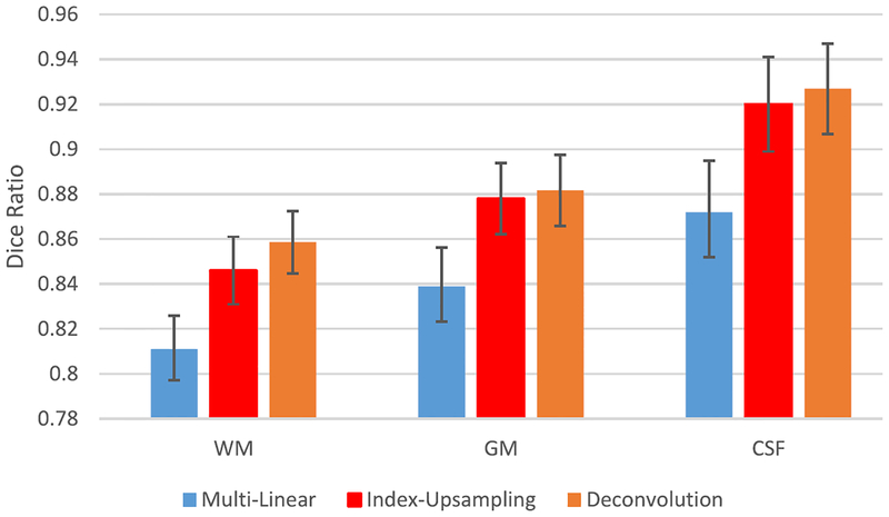
I. Impact of Upsampling Strategies
Upsampling layers (e.g., deconvolution layer in our proposed model) play an important role in the deep learning-based segmentation models. Thus, we conduct experiments to investigate different upsampling strategies.
“Multilinear” (using multilinear interpolation to upsample the input feature maps).
“Deconvolution” (upsampling by learning to deconvolve the input feature map) [26].
“Index-upsampling” (using the max pooling indices to upsample (without learning) the feature map(s) and convolve with a bank of trainable filters) [38].
Note, all the other settings are the same, except that we use different upsampling strategies for the comparison experiments. The comparison experimental results are shown in Fig. 11, indicating that deconvolution works best, and index-upsampling provides close performance to deconvolution, while multilinear interpolation leads to the worst results. Thus, we select deconvolution in our experiment.
Fig. 11.
Segmentation performance with respect to the use of different upsampling strategies for the proposed model.
J. Patch Merging Strategy
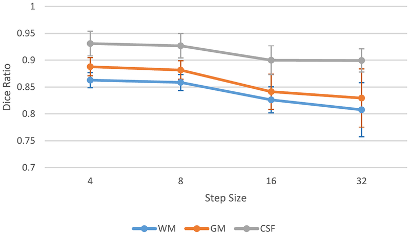
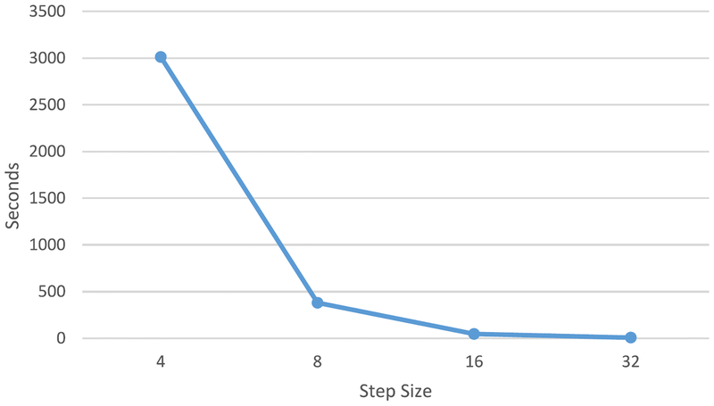
The CC-3-D-FCN is trained in a patch level. In the testing stage, we have to first partition a whole image (T1, T2, and FA) into overlapping or nonoverlapping patches, and then feed these patches into trained networks. The corresponding output patches are further merged to form a fully predicted label map. It is worth noting that the extent of patch overlapping can largely affect the final performance, in terms of both segmentation accuracy and computational complexity. We explore the extent of patch overlapping in the testing stage. Specifically, we extract the patches from MR images with a step size of 32 (nonoverlapping), 16, 8, and 4. After these patches are fed into the trained model, all the predicted label patches from the same subject are combined into a single label image by averaging the label values of the overlapping image regions. The performance, in terms of Dice ratio and time cost, are given in Figs. 12 and 13, respectively.
Fig. 12.
Changes of Dice ratios of WM, GM, and CSF on 11 isointense subjects, with respect to different step size at the testing stage. Leave-one-subject-out cross validation is used.
Fig. 13.
Changes of average time cost of tissue segmentation for one subject, with respect to different step size at the testing stage.
As shown by both figures (Figs. 12 and 13), the smaller the step size, the better the segmentation accuracy. This is because we can average over more predicted labels when the step size is smaller. However, small step size brings heavy work load and makes the computational cost increase dramatically. To this end, we conduct a tradeoff between computational cost and prediction accuracy, and finally select the step size as 8 for the testing stage.
K. Experimental Results on the First Dataset
We first conduct experiments on the first dataset containing three imaging modalities (T1, T2, and FA). The proposed CC-3-D-FCN is used to perform voxel-wise tissue segmentation with a leave-one-subject-out strategy. It takes approximately 130 h to train our designed neural networks on a Titan × GPU.
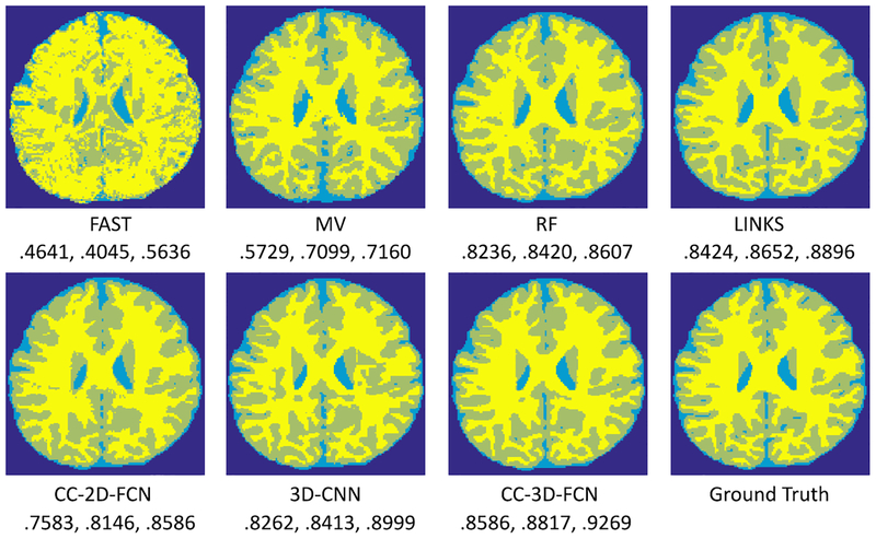
To qualitatively demonstrate the advantage of the proposed CC-3-D-FCN on this dataset, we first show the segmentation results of different tissues for a typical subject in Fig. 14.
Fig. 14.
Comparison of segmentation results by different methods, along with manual ground truth on a typical infant subject as shown in Fig. 1. The Dice ratios for WM, GM, and CSF are listed below each method, respectively.
To quantitatively evaluate segmentation performance, we use Dice ratio to measure the overlap ratio between automated and manual segmentation results. We report the segmentation performance in Table I. We can observe that CC-3-D-FCN outperforms other methods (p= 0.0371, performed by a paired t-test). Specifically, CC-3-D-FCN could achieve the average Dice ratios of 0.9269 for CSF, 0.8817 for GM, and 0.8586 for WM, from these 11 subjects. In contrast, one of the state-of-the-art methods, i.e., RF with auto-context model (LINKS) [52], achieved the overall Dice ratios of 0.8896, 0.8652, and 0.8424 for CSF, GM, and WM, respectively.
TABLE I.
Segmentation Performance in Terms of Dice Ratio and Standard Deviation, Achieved by the Baseline Comparison Methods and Our CC-3-D-FCN on 11 Subjects. The Highest Performance in Each Tissue Class Is Highlighted in Bold
| WM | GM | CSF | |
|---|---|---|---|
| FAST | .4641(.0791) | .4045(.0979) | .5636(.2334) |
| MV | .5729(.0327) | .7099(.0412) | .7160(.0386) |
| RF | .8236(.0164) | .8420(.0126) | .8607(.0170) |
| LINKS | .8424(.0183) | .8652(.0154) | .8896(.0251) |
| DeepMedic [54] | .8458(.0150) | .8608(.0158) | .9196(.0210) |
| 3D-UNet [55] | .8418(.0161) | .8680(.0172) | .9012(.0225) |
| CC-2D-FCN | .7583(.0215) | .8146(.0115) | .8586(.0101) |
| 3D-CNN | .8262(.0242) | .8413(0.0329) | .8999(.0269) |
| CC-3D-FCN | .8586(.0139) | .8817(.0158) | .9269(.0201) |
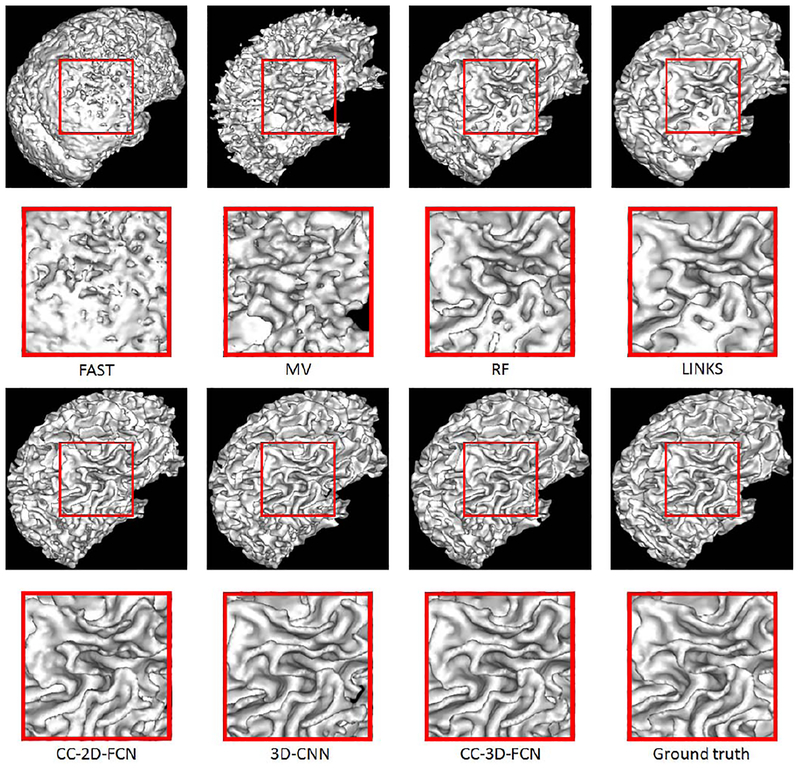
We also provide WM surfaces obtained by different methods in Fig. 15. These WM surfaces qualitatively demonstrate the advantage of our proposed method, as it achieves the best visual results.
Fig. 15.
Comparison of WM surfaces obtained by different methods on a typical subject shown in Fig. 1.
The MHD comparison is also shown in Table II. It can be seen again that our proposed method produces a competitive accuracy compared to all the state-of-the-art methods.
TABLE II.
Segmentation Performance in Terms of MHD and Standard Deviation, Achieved by the Baseline Comparison Methods and Our CC-3-D-FCN on 11 Subjects. The Highest Performance in Each Tissue Class Is Highlighted in Bold
| WM | GM | CSF | |
|---|---|---|---|
| FAST | 1.7052(.0092) | 1.0083(.0269) | 1.8276(.0882) |
| MV | 1.7204(.4780) | 1.1840(. 1639) | 1.9323(.2075) |
| RF | .6837(.0893) | .5625(.0502) | .4624(.0669) |
| LINKS | .5659(.0794) | .4827(.0460) | .3321(.0426) |
| DeepMedic [54] | .5154(.0540) | .4878(.0414) | .3621(.0495) |
| 3D-UNet [55] | .5951(.0488) | .4420(.0415) | .3630(.0488) |
| CC-2D-FCN | .7773(.1907) | .6011(.1082) | .5379(.1210) |
| 3D-CNN | .5802(.1386) | .4967(.0839) | .3561(.0817) |
| CC-3D-FCN | .3423(.0358) | .3108(.0256) | .3230(.0788) |
L. Comparison of 3-D- and 2-D-Based FCN
As medical image data is often acquired in 3-D, 3-D operations are assumed to offer better performance than 2-D operations. So, it is important to highlight how the 3-D architecture improves the performance, compared to the conventional 2-D architectures. Specifically, we run our model with exactly same architecture, but with all 2-D filters, and then provide results in Table I. As can be seen, the 3-D model performs approximately 11% better than the 2-D approach. This advantage comes from the fact that 3-D convolution filters can consider the 3-D structures, as input images are in 3-D. Thus, 3-D operations can model much better internal structures. Furthermore, adopting 3-D operations can avoid inconsistency in the third dimension of the images, which is usually a problem when simply applying 2-D filters to the 3-D images.
M. Time and Computational Complexity
As the model training can be completed offline, the testing time cost is often more important for a segmentation task. Thus, in Table III, we provide the average time cost of segmenting one test subject by each segmentation approach. Note that this experiment is performed on the same PC with the following settings—memory: 16-GB Quad Channel DDR4; video card: Nvidia Titan X; processor: Intel i7–5820K; and operation system: Ubuntu 14.04. The running time in minutes are listed in Table III for different segmentation methods. As can be seen, our proposed CC-3-D-FCN method is significantly faster than any of the other methods.
TABLE III.
Average Time Cost (in Minutes) of Each Test Subject and Standard Deviation, by the Baseline Comparison Methods and Our Proposed CC-3-D-FCN on 11 Subjects in the First Dataset
N. Results on the Second Dataset
To show the generalization ability of our proposed 3-D-CC-FCN architecture, we further conduct experiments on the second large dataset with other 50 isointense-phase subjects which were obtained from the NIH-supported National Database for Autism Research (NDAR), where each subject has both T1 and T2 images, but no FA images. Fivefold cross validation is performed. Note that, in each fold, it takes approximately 25 h to train our designed neural networks on a Titan × GPU.
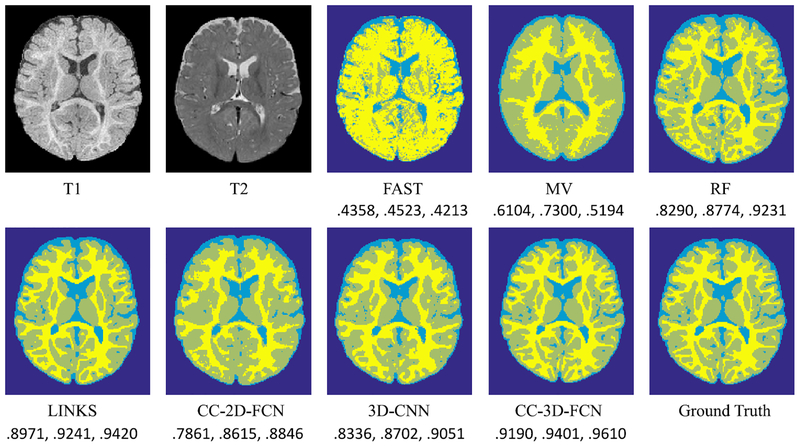
In Fig. 16, we show the segmentation results by different methods a typical subject in the second dataset. To quantitatively evaluate segmentation performance, we report Dice ratios in Table IV.
Fig. 16.
Comparison of segmentation results by baseline comparison methods and our proposed CC-3-D-FCN, along with manual ground truth, on a typical subject in the second dataset. The Dice ratios for WM, GM, and CSF are listed below each method, respectively.
TABLE IV.
Segmentation Performance in Terms of Dice Ratio and Standard Deviation, Obtained by the Baseline Comparison Methods and Our Proposed CC-3-D-FCN on 50 Subjects. The Highest Performance in Each Tissue Class Is Highlighted in Bold
| WM | GM | CSF | |
|---|---|---|---|
| FAST | .4358(.0903) | .4523(.1397) | .4213(3282) |
| MV | .6104(.0163) | .7300(.0196) | .5194(.0316) |
| RF | .8290(.0150) | .8774(.0059) | .9231(.0127) |
| LINKS | .8971(.0074) | .9241(.0043) | .9420(.0074) |
| DeepMedic [54] | .8943(.0088) | .9265(.0051) | .9484(.0086) |
| 3D-UNet [55] | .8907(.0087) | .9228(.0049) | .9465(.0095) |
| CC-2D-FCN | .7861(.0240) | .8615(.0080) | .8846(.0177) |
| 3D-CNN | .8336(.0177) | .8702(.0070) | .9051(.0168) |
| CC-3D-FCN | .9190(.0085) | .9401(.0052) | .9610(.0090) |
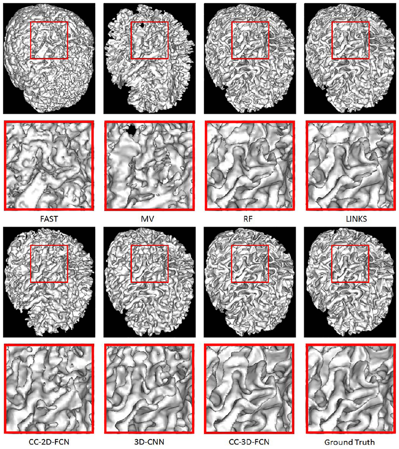
As shown in Table IV, our proposed CC-3-D-FCN again achieves the best performance in segmenting WM (0.9190±0.0085), GM (0.9401±0.0052), and CSF (0.9610±0.0090), compared to the state-of-the-art method [52] which uses multiscale RF and auto-context model to take advantage of multisource information and refine the results. Our proposed CC-3-D-FCN also outperforms the conventional CNN, indicating that our CC-3-D-FCN is more capable in this segmentation task. Furthermore, our proposed CC-3-D-FCN works better than CC-2-D-FCN in all three tissues, indicating that 3-D deep learning architectures are better for 3-D segmentation tasks than the 2-D deep learning architectures. We also provide WM surfaces obtained by different segmentation methods in Fig. 17, which further demonstrates the advantage of our proposed CC-3-D-FCN. Moreover, the MHD comparison is further provided in Table V, where our proposed CC-3-D-FCN produces less errors compared to all the state-of-the-art methods.
Fig. 17.
Comparison of WM surfaces obtained with different methods on a typical subject (of the second dataset) shown in Fig. 16.
TABLE V.
Segmentation Performance in Terms of MHD and Standard Deviation, Obtained by the Baseline Comparison Methods and Our Proposed CC-3-D-FCN on 50 Subjects. The Highest Performance in Each Tissue Class Is Highlighted in Bold
| WM | GM | CSF | |
|---|---|---|---|
| FAST | 1.7161(.2884) | 1.0184(.3712) | 1.1053(.5241) |
| MV | 1.4101(.0841) | 1.0962(.2187) | 1.3438(.6356) |
| RF | .7757(.0571) | .6513(.0321) | .3090(.0250) |
| LINKS | .4515(.0217) | .3961(.0108) | .2565(.0282) |
| DeepMedic [54] | .4601(.0303) | .3990(.0210) | .2736(.02922) |
| 3D-UNet [55] | .4948(.0230) | .4003(.0119) | .2285(.0187) |
| CC-2D-FCN | .8424(.0373) | .8766(.0424) | .9300(.0138) |
| 3D-CNN | .6867(.0443) | .6912(.0576) | .7401(.0756) |
| CC-3D-FCN | .3676(.0223) | .3530(.0110) | .1890(.0122) |
O. Limitation of Our Proposed Method
The main problem of our proposed method is that the segmented infant brain images are a little bit smooth, especially for the tissues near the boundaries, as shown in Figs. 14 and 16. This is mainly due to the use of convolution and pooling in the ConvNets. On the other hand, although we can get high localization accuracy because of using local image patch, we miss global context information to guide the spatial consistency of tissue segmentation. This is because patch size is much smaller compared to the whole image size, and thus we cannot use the whole image information to train our model; on the other hand, if using the whole image for training, the number of training images is too small to train our neural network. We will investigate these two issues in our future work.
IV. Conclusion
In this paper, we have proposed CC-3-D-FCN to segment isointense-phase brain images with multimodality MR images. In our designed deep learning model, we integrate coarse layer information with dense layer information to refine the segmentation performance. We also propose to use an additional convolutional layer to solve the biased signals problem. Furthermore, we propose to employ BN to make the networks converge faster and better. We have also trained our CC-3-DFCN in an end-to-end and voxel-to-voxel manner to achieve voxel-level segmentation. With largely reduced parameters, our method is also easier and faster to train. We have compared our proposed method with several commonly used segmentation methods, along with state-of-the-art methods, and the experimental results show that our proposed method outperforms all comparison methods on isointense-phase brain segmentation, in terms of both segmentation accuracy and time cost. Moreover, our proposed method also presents a novel way of fusing multilayer information to better conduct brain tissue segmentation.
Acknowledgment
This paper reflects the views of the authors and may not reflect the opinions or views of the NIH or of the submitters submitting original data to National Database for Autism Research.
Manuscript received December 5, 2016; revised November 20, 2017, January 15, 2018, and January 18, 2018; accepted January 19, 2018. This work was supported in part by the National Institutes of Health under Grant MH109773, Grant MH100217, Grant MH070890, Grant EB006733, Grant EB008374, Grant EB009634, Grant AG041721, Grant AG042599, and Grant MH088520, and in part by the NIH-supported National Database for Autism Research. This paper was recommended by Associate Editor M. Shin.
Biographies

Dong Nie received the B.Eng. degree in computer science from Northeastern University, Shenyang, China, and the M.Sc. degree in computer science from the University of Chinese Academy of Sciences, Beijing, China. He is currently pursuing the Ph.D. degree in computer science from the University of North Carolina at Chapel Hill, Chapel Hill, NC, USA.
His current research interests include image processing, medical image analysis, and natural language processing.
Li Wang received the Ph.D. degree in pattern recognition and intelligent system from Nanjing University of Science and Technology, Nanjing, China, in 2010.
He is currently a Research Assistant Professor with the University of North Carolina at Chapel Hill, Chapel Hill, NC, USA. His current research interests include image segmentation, image registration, cortical surface analysis, machine learning, and their applications to normal early brain development and disorders.

Ehsan Adeli received the Ph.D. degree from the Iran University of Science and Technology, Tehran, Iran.
He is a Post-Doctoral Research Fellow with Stanford University, Stanford, CA, USA. He was a Post-Doctoral Researcher with the University of North Carolina at Chapel Hill, Chapel Hill, NC, USA. He was a Visiting Research Scholar with the Robotics Institute, Carnegie Mellon University, Pittsburgh, PA, USA. His current research interests include machine learning, computer vision, medical image analysis, and computational neuroscience.

Cuijin Lao received the B.Eng. degree in computer science from the Guilin University of Electronic Technology, Guilin, China, in 2002, and the M.Sc. degree in education from Guangxi Normal University, Guilin, in 2008.
She is with Liuzhou City Vocational College, Liuzhou, China. Her current research interests include image processing, computer education, and computer network.

Weili Lin received the Ph.D. degree in Biomedical Engineering from Case Western Reserve University, Cleveland, OH, USA, in 1993.
He is currently the Director of the Biomedical Research Imaging Center, a Dixie Lee Boney Soo Distinguished Professor of Neurological Medicine, and the Vice Chair of the Department of Radiology, University of North Carolina at Chapel Hill, Chapel Hill, NC, USA. His current research interests include cerebral ischemia, human brain development, PET, and magnetic resonance.

Dinggang Shen (F’18) received the Ph.D. degree in electrical engineering from Shanghai Jiao Tong University, Shanghai, China, in 1995.
He is a Jeffrey Houpt Distinguished Investigator, and a Professor with the Radiology, Biomedical Research Imaging Center (BRIC), Computer Science, and Biomedical Engineering, University of North Carolina at Chapel Hill, Chapel Hill, NC, USA, where he is also currently directing the Center for Image Analysis and Informatics, Image Display, Enhancement, and Analysis Laboratory, Department of Radiology, and also the medical image analysis core in the BRIC. He was a tenure-track Assistant Professor with the University of Pennsylvania, Philadelphia, PA, USA, and a Faculty Member with Johns Hopkins University, Baltimore, MD, USA. He has published over 800 papers in the international journals and conference proceedings. His current research interests include medical image analysis, computer vision, and pattern recognition.
Mr. Shen serves as an Editorial Board Member for eight international journals. He has also served in the Board of Directors, the Medical Image Computing and Computer Assisted Intervention Society from 2012 to 2015. He is a fellow of the American Institute for Medical and Biological Engineering.
Footnotes
Contributor Information
Dong Nie, Department of Computer Science, University of North Carolina at Chapel Hill, Chapel Hill, NC 27510 USA,; Department of Radiology and Biomedical Research Imaging Center, University of North Carolina at Chapel Hill, Chapel Hill, NC 27510 USA.
Li Wang, Department of Radiology and Biomedical Research Imaging Center, University of North Carolina at Chapel Hill, Chapel Hill, NC 27510 USA..
Ehsan Adeli, Department of Radiology and Biomedical Research Imaging Center, University of North Carolina at Chapel Hill, Chapel Hill, NC 27510 USA..
Cuijin Lao, Department of Radiology and Biomedical Research Imaging Center, University of North Carolina at Chapel Hill, Chapel Hill, NC 27510 USA..
Weili Lin, Department of Radiology and Biomedical Research Imaging Center, University of North Carolina at Chapel Hill, Chapel Hill, NC 27510 USA..
Dinggang Shen, Department of Radiology and Biomedical Research Imaging Center, University of North Carolina at Chapel Hill, Chapel Hill, NC 27510 USA,; Department of Brain and Cognitive Engineering, Korea University, Seoul 02841, South Korea
References
- [1].Li G et al. , “Mapping longitudinal development of local cortical gyrification in infants from birth to 2 years of age,” J. Neurosci, vol. 34, no. 12, pp. 4228–4238, 2014. [DOI] [PMC free article] [PubMed] [Google Scholar]
- [2].Hazlett HC et al. , “Early brain overgrowth in autism associated with an increase in cortical surface area before age 2 years,” Archives Gen. Psychiat, vol. 68, no. 5, pp. 467–476, 2011. [DOI] [PMC free article] [PubMed] [Google Scholar]
- [3].Lyall AE et al. , “Dynamic development of regional cortical thickness and surface area in early childhood,” Cerebral Cortex, vol. 25, no. 8, pp. 2204–2212, 2014. [DOI] [PMC free article] [PubMed] [Google Scholar]
- [4].Gao W et al. , “The synchronization within and interaction between the default and dorsal attention networks in early infancy,” Cerebral Cortex, vol. 23, no. 3, pp. 594–603, 2012. [DOI] [PMC free article] [PubMed] [Google Scholar]
- [5].Knickmeyer RC et al. , “A structural MRI study of human brain development from birth to 2 years,” J. Neurosci, vol. 28, no. 47, pp. 12176–12182, 2008. [DOI] [PMC free article] [PubMed] [Google Scholar]
- [6].Gilmore JH et al. , “Longitudinal development of cortical and subcortical gray matter from birth to 2 years,” Cerebral Cortex, vol. 22, no. 11, pp. 2478–2485, 2012. [DOI] [PMC free article] [PubMed] [Google Scholar]
- [7].Li G et al. , “Mapping region-specific longitudinal cortical surface expansion from birth to 2 years of age,” Cerebral Cortex, vol. 23, no. 11, pp. 2724–2733, 2013. [DOI] [PMC free article] [PubMed] [Google Scholar]
- [8].Li G, Wang L, Shi F, Lin W, and Shen D, “Constructing 4D infant cortical surface atlases based on dynamic developmental trajectories of the cortex,” in Proc. Int. Conf. Med. Image Comput. Comput. Assisted Intervent., 2014, pp. 89–96. [DOI] [PMC free article] [PubMed] [Google Scholar]
- [9].Weisenfeld NI and Warfield SK, “Automatic segmentation of newborn brain MRI,” Neuroimage, vol. 47, no. 2, pp. 564–572, 2009. [DOI] [PMC free article] [PubMed] [Google Scholar]
- [10].Xue H et al. , “Automatic segmentation and reconstruction of the cortex from neonatal MRI,” Neuroimage, vol. 38, no. 3, pp. 461–477, 2007. [DOI] [PubMed] [Google Scholar]
- [11].Gui L et al. , “Morphology-driven automatic segmentation of MR images of the neonatal brain,” Med. Image Anal, vol. 16, no. 8, pp. 1565–1579, 2012. [DOI] [PubMed] [Google Scholar]
- [12].Pham DL, Xu C, and Prince JL, “Current methods in medical image segmentation 1,” Annu. Rev. Biomed. Eng, vol. 2, no. 1, pp. 315–337, 2000. [DOI] [PubMed] [Google Scholar]
- [13].Prastawa M, Gilmore JH, Lin W, and Gerig G, “Automatic segmentation of MR images of the developing newborn brain,” Med. Image Anal, vol. 9, no. 5, pp. 457–466, 2005. [DOI] [PubMed] [Google Scholar]
- [14].Warfield SK, Kaus M, Jolesz FA, and Kikinis R, “Adaptive, template moderated, spatially varying statistical classification,” Med. Image Anal, vol. 4, no. 1, pp. 43–55, 2000. [DOI] [PubMed] [Google Scholar]
- [15].Wang L et al. , “Segmentation of neonatal brain MR images using patch-driven level sets,” NeuroImage, vol. 84, pp. 141–158, Jan. 2014. [DOI] [PMC free article] [PubMed] [Google Scholar]
- [16].Anbeek P et al. , “Probabilistic brain tissue segmentation in neonatal magnetic resonance imaging,” Pediatric Res, vol. 63, no. 2, pp. 158–163, 2008. [DOI] [PubMed] [Google Scholar]
- [17].Leroy F et al. , “Atlas-free surface reconstruction of the cortical grey-white interface in infants,” PloS ONE, vol. 6, no. 11, 2011, Art. no. e27128. [DOI] [PMC free article] [PubMed] [Google Scholar]
- [18].Shi F et al. , “Construction of multi-region-multi-reference atlases for neonatal brain MRI segmentation,” Neuroimage, vol. 51, no. 2, pp. 684–693, 2010. [DOI] [PMC free article] [PubMed] [Google Scholar]
- [19].Shi F, Yap P-T, Gilmore JH, Lin W, and Shen D, “Spatial-temporal constraint for segmentation of serial infant brain MR images,” in Proc. Int. Workshop Med. Imag. Virtual Reality, 2010, pp. 42–50. [Google Scholar]
- [20].Wang L et al. , “4D multi-modality tissue segmentation of serial infant images,” PLoS ONE, vol. 7, no. 9, 2012, Art. no. e44596. [DOI] [PMC free article] [PubMed] [Google Scholar]
- [21].Kim SH et al. , “Adaptive prior probability and spatial temporal intensity change estimation for segmentation of the one-year-old human brain,” J. Neurosci. Methods, vol. 212, no. 1, pp. 43–55, 2013. [DOI] [PMC free article] [PubMed] [Google Scholar]
- [22].Zhang W et al. , “Deep convolutional neural networks for multi-modality isointense infant brain image segmentation,” NeuroImage, vol. 108, pp. 214–224, Mar. 2015. [DOI] [PMC free article] [PubMed] [Google Scholar]
- [23].Moeskops P et al. , “Automatic segmentation of MR brain images with a convolutional neural network,” IEEE Trans. Med. Imag, vol. 35, no. 5, pp. 1252–1261, May 2016. [DOI] [PubMed] [Google Scholar]
- [24].Nie D, Wang L, Gao Y, and Sken D, “Fully convolutional networks for multi-modality isointense infant brain image segmentation,” in Proc. IEEE 13th Int. Symp. Biomed. Imag. (ISBI), 2016, pp. 1342–1345. [DOI] [PMC free article] [PubMed] [Google Scholar]
- [25].Chen H, Dou Q, Yu L, Qin J, and Heng PA, “VoxResNet: Deep voxelwise residual networks for brain segmentation from 3D MR images,” NeuroImage, Apr. 2017. [DOI] [PubMed] [Google Scholar]
- [26].Long J, Shelhamer E, and Darrell T, “Fully convolutional networks for semantic segmentation,” in Proc. IEEE Conf. Comput. Vis. Pattern Recognit., Boston, MA, USA, 2015, pp. 3431–3440. [DOI] [PubMed] [Google Scholar]
- [27].Chen L-C, Papandreou G, Kokkinos I, Murphy K, and Yuille AL, “Semantic image segmentation with deep convolutional nets and fully connected CRFs,” in Proc. ICLR, San Diego, CA, USA, May 2015. [DOI] [PubMed] [Google Scholar]
- [28].Ronneberger O, Fischer P, and Brox T, “U-net: Convolutional networks for biomedical image segmentation,” in Proc. Int. Conf. Med. Image Comput. Comput. Assisted Intervent., 2015, pp. 234–241. [Google Scholar]
- [29].He K, Zhang X, Ren S, and Sun J, “Deep residual learning for image recognition,” in Proc. IEEE Conf. Comput. Vis. Pattern Recogn., 2016, pp. 770–778. [Google Scholar]
- [30].Szegedy C et al. , “Going deeper with convolutions,” in Proc. IEEE Conf. Comput. Vis. Pattern Recognit., Boston, MA, USA, 2015, pp. 1–9. [Google Scholar]
- [31].Krizhevsky A, Sutskever I, and Hinton GE, “ImageNet classification with deep convolutional neural networks,” in Proc. Adv. Neural Inf. Process. Syst., 2012, pp. 1097–1105. [Google Scholar]
- [32].Simonyan K and Zisserman A, “Very deep convolutional networks for large-scale image recognition,” in Proc. ICLR, San Diego, CA, USA, May 2015. [Google Scholar]
- [33].LeCun Y, Bottou L, Bengio Y, and Haffner P, “Gradient-based learning applied to document recognition,” Proc. IEEE, vol. 86, no. 11, pp. 2278–2324, Nov. 1998. [Google Scholar]
- [34].Ji S, Xu W, Yang M, and Yu K, “3D convolutional neural networks for human action recognition,” IEEE Trans. Pattern Anal. Mach. Intell, vol. 35, no. 1, pp. 221–231, Jan. 2013. [DOI] [PubMed] [Google Scholar]
- [35].Ciresan DC, Giusti A, Gambardella LM, and Schmidhuber J, “Deep neural networks segment neuronal membranes in electron microscopy images,” in Proc. Adv. Neural Inf. Process. Syst., 2012, pp. 2843–2851. [Google Scholar]
- [36].Farabet C, Couprie C, Najman L, and LeCun Y, “Learning hierarchical features for scene labeling,” IEEE Trans. Pattern Anal. Mach. Intell, vol. 35, no. 8, pp. 1915–1929, Aug. 2013. [DOI] [PubMed] [Google Scholar]
- [37].Pinheiro PHO and Collobert R, “Recurrent convolutional neural networks for scene labeling,” in Proc. ICML, Beijing, China, 2014, pp. 82–90. [Google Scholar]
- [38].Badrinarayanan V, Kendall A, and Cipolla R, “SegNet: A deep convolutional encoder-decoder architecture for image segmentation,” IEEE Trans. Pattern Anal. Mach. Intell, vol. 39, no. 12, pp. 2481–2495, Dec. 2017. [DOI] [PubMed] [Google Scholar]
- [39].Wang L et al. , “Integration of sparse multi-modality representation and anatomical constraint for isointense infant brain MR image segmentation,” NeuroImage, vol. 89, pp. 152–164, Apr. 2014. [DOI] [PMC free article] [PubMed] [Google Scholar]
- [40].Nair V and Hinton GE, “Rectified linear units improve restricted Boltzmann machines,” in Proc. 27th Int. Conf. Mach. Learn. (ICML), Haifa, Israel, 2010, pp. 807–814. [Google Scholar]
- [41].Eigen D, Puhrsch C, and Fergus R, “Depth map prediction from a single image using a multi-scale deep network,” in Proc. Adv. Neural Inf. Process. Syst., Montreal, QC, Canada, 2014, pp. 2366–2374. [Google Scholar]
- [42].Ioffe S and Szegedy C, “Batch normalization: Accelerating deep network training by reducing internal covariate shift,” in Proc. Int. Conf. Mach. Learn., 2015, pp. 448–456. [Google Scholar]
- [43].Dou Q et al. , “3D deeply supervised network for automatic liver segmentation from CT volumes,” in Proc. Int. Conf. Med. Image Comput. Comput. Assist. Intervention, 2016, pp. 149–157. [Google Scholar]
- [44].Glorot X and Bengio Y, “Understanding the difficulty of training deep feedforward neural networks,” in Proc. Int. Conf. Artif. Intell. Stat., 2010, pp. 249–256. [Google Scholar]
- [45].Bell S, Zitnick CL, Bala K, and Girshick R, “Inside-outside net: Detecting objects in context with skip pooling and recurrent neural networks,” in Proc. IEEE Conf. Comput. Vis. Pattern Recogn., 2016, pp. 2874–2883. [Google Scholar]
- [46].LeCun Y, Bottou L, Orr GB, and Müller KR, “Efficient backprop,” in Neural Networks: Tricks of the Trade. Berlin, Germany: Springer, 1998, pp. 9–50. [Google Scholar]
- [47].Jia Y et al. , “Caffe: Convolutional architecture for fast feature embedding,” in Proc. ACM Int. Conf. Multimedia, Orlando, FL, USA, 2014, pp. 675–678. [Google Scholar]
- [48].Dai Y, Shi F, Wang L, Wu G, and Shen D, “iBEAT: A toolbox for infant brain magnetic resonance image processing,” Neuroinformatics, vol. 11, no. 2, pp. 211–225, 2013. [DOI] [PubMed] [Google Scholar]
- [49].Dubuisson M-P and Jain AK, “A modified Hausdorff distance for object matching,” in Proc. 12th IAPR Int. Conf. Pattern Recognit. Vol. 1 Conf. A Comput. Vis. Amp Image Process., vol. 1 1994, pp. 566–568. [Google Scholar]
- [50].Zhang Y, Brady M, and Smith S, “Segmentation of brain MR images through a hidden Markov random field model and the expectation-maximization algorithm,” IEEE Trans. Med. Imag, vol. 20, no. 1, pp. 45–57, Jan. 2001. [DOI] [PubMed] [Google Scholar]
- [51].Avants BB, Epstein CL, Grossman M, and Gee JC, “Symmetric diffeomorphic image registration with cross-correlation: Evaluating automated labeling of elderly and neurodegenerative brain,” Med. Image Anal, vol. 12, no. 1, pp. 26–41, 2008. [DOI] [PMC free article] [PubMed] [Google Scholar]
- [52].Wang L et al. , “LINKS: Learning-based multi-source integration framework for segmentation of infant brain images,” NeuroImage, vol. 108, pp. 160–172, Mar. 2015. [DOI] [PMC free article] [PubMed] [Google Scholar]
- [53].Ngiam J et al. , “Multimodal deep learning,” in Proc. 28th Int. Conf. Mach. Learn. (ICML), 2011, pp. 689–696. [Google Scholar]
- [54].Kamnitsas K et al. , “Efficient multi-scale 3D CNN with fully connected CRF for accurate brain lesion segmentation,” Med. Image Anal, vol. 36, pp. 61–78, Feb. 2017. [DOI] [PubMed] [Google Scholar]
- [55].Çiçek Ö, Abdulkadir A, Lienkamp SS, Brox T, and Ronneberger O, “3D U-NET: Learning dense volumetric segmentation from sparse annotation,” in Proc. Int. Conf. Med. Image Comput. Comput. Assisted Intervent., 2016, pp. 424–432. [Google Scholar]


