Retrospective harmonization of multi-site diffusion MRI data acquired with different acquisition parameters

Abstract

A joint and integrated analysis of multi-site diffusion MRI (dMRI) datasets can dramatically increase the statistical power of neuroimaging studies and enable comparative studies pertaining to several brain disorders. However, dMRI data sets acquired on multiple scanners cannot be naively pooled for joint analysis due to scanner specific nonlinear effects as well as differences in acquisition parameters. Consequently, for joint analysis, the dMRI data has to be harmonized, which involves removing scanner-specific differences from the raw dMRI signal. In this work, we propose a dMRI harmonization method that is capable of removing scanner-specific effects, while accounting for minor differences in acquisition parameters such as b-value, spatial resolution and number of gradient directions. We validate our algorithm on dMRI data acquired from two sites: Philadelphia Neuro-developmental Cohort (PNC) with 800 healthy adolescents (ages 8–22 years) and Brigham and Women’s Hospital (BWH) with 70 healthy subjects (ages 14–54 years). In particular, we show that gender and age-related maturation differences in different age groups are preserved after harmonization, as measured using effect sizes (small, medium and large), irrespective of the test sample size. Since we use matched control subjects from different scanners to estimate scanner-specific effects, our goal in this work is also to determine the minimum number of well-matched subjects needed from each site to achieve best harmonization results. Our results indicate that at-least 16 to 18 well-matched healthy controls from each site are needed to reliably capture scanner related differences. The proposed method can thus be used for retrospective harmonization of raw dMRI data across sites despite differences in acquisition parameters, while preserving inter-subject anatomical variability.

1. Introduction

The sensitivity of diffusion MRI to microscopic molecular motion forms the foundation to study the neural architecture of the brain. However, these measurements are affected by different hardware specifications (magnetic field strength, number of receiver coils etc.), and different acquisition parameters (echo time, diffusion time, gradient strength, voxel size, number of gradient directions etc.) (Helmer et al., 2016). Therefore, the data acquired by each scanner is substantially different even for the same subject. In fact, even if the same subject is scanned with the same hardware from the same manufacturer, diffusion signal can still be different (Vollmar et al., 2010). This is due to differences in magnetic field inhomogeneities, sensitivity of receiver coils, the number of receiver coils used, vendor-specific MRI reconstruction algorithms and differences in acquisition parameters. Consequently, dMRI data must be harmonized prior to joint analysis.

Several methods have characterized both intra-scanner and inter-scanner variability in structural and dMRI data (Landman et al., 2011, 2007). Based on their study in Walker et al. (2013), the authors recommend the use of physical phantoms to monitor and quickly detect any scanner-related changes in ongoing neuroimaging studies. While the use of physical phantoms is necessary, they are inadequate in capturing the regional and tissue specific scanner differences. Further, it is non-trivial to use the scanner differences observed in physical phantoms to correct human in-vivo data, due to the complexities of biological tissue.

Existing techniques on data pooling or harmonization are based on using diffusion tensor imaging (DTI) derived metrics (Salimi-Khorshidi et al., 2009; Jahanshad et al., 2013; Kochunov et al., 2014; Forsyth et al., 2014; Venkatraman et al., 2015; Jenkins et al., 2016; Pohl et al., 2016; Fortin et al., 2017). For instance, Salimi-Khorshidi et al. (2009); Jahanshad et al. (2013); Kochunov et al. (2014); Palacios et al. (2016); Kelly et al. (2017) use meta-analysis approach which involves combining z-scores of a given diffusion measure (e.g. fractional anisotropy (FA)) from all sites to determine group differences. However, the subject population at each site may not be sufficient to capture the variance of the entire population, a critical requirement to ensure proper pooling and analysis of the z-scores (which depends on the variance and not just the population mean). Further, z-scores may not be the best statistic to use if the distribution of the diffusion measure in the population is not Gaussian (normal). On the other hand, Forsyth et al. (2014); Venkatraman et al. (2015); Fortin et al. (2017) use statistical covariates to regress out the differences between sites in DTI measures such as FA, mean diffusivity (MD) or cortical thickness. Of particular note is the work of Pohl et al. (2016), where the authors use information from 3 traveling subjects to obtain a linear correction factor for scanner related effects in FA (a different correction factor for each ROI analyzed). This method however has limitations when using large ROIs (such as the corticospinal tract), as the scanner-related effects are not only non-linear but also regionally varying (see (Mirzaalian et al., 2016) and Fig. 2). Thus, due to the regional variability of the diffusion signal, using a single regressor for large ROIs can lead to erroneous results in the aggregated data (Mirzaalian et al., 2016; Fortin et al., 2017). Further, it is also well known that the differences in the signal-to-noise ratio (SNR) of the acquisitions at each site might add to variability in the estimated dMRI parameters such as FA (Farrell et al., 2007).

Fig. 2.

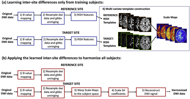
Steps of multi-variate RISH feature template construction and dMRI data harmonization.

All of the methods mentioned above have to correct for scanner-specific effects in each diffusion measure of interest separately, i.e., a linear correction factor for each diffusion measure, thus making the harmonization procedure entirely model-specific (e.g. single tensor). Recently, Fortin et al. (2017) have proposed a powerful and fast statistical data pooling tool that uses ComBat (a batch-effect correction tool used in genomics) for retrospective data harmonization. This method estimates an additive and a multiplicative site-effect coefficient at each voxel, thus accounting for regional scanner differences. ComBat works on the finalized parameter maps, and in practice can be applied to any parameter map (e.g. FA, MD, mean kurtosis, etc). Despite this, their optimization procedure assumes that the site-effect parameters follow a particular parametric prior distribution (Gaussian and Inverse-gamma), which might not generalize to all scenarios or measures derived from other models (e.g., multi-compartment models). Besides, it is not clear how the nonlinearities in the signal due site-effect propagate through the preprocessing techniques as well as the model fitting procedures.

1.1. Contributions of this work

In our earlier works (Mirzaalian et al., 2016, 2017), we had proposed a model-free dMRI harmonization method which can be used to harmonize the “raw dMRI signal” (and not just a particular dMRI measure of interest) across sites. However, that work exclusively focused on harmonizing dMRI data across sites but with similar acquisition parameters. Thus, the method worked only when the spatial resolution and b-values were the same across sites. Additionally, the earlier method did not have an extensive validation on a large dataset.

In this work, we further build on our existing framework and propose a model free harmonization method that learns an efficient mapping across scanners despite differences in scanner parameters. We extensively validate our algorithm on dMRI data acquired from two different sites with different acquisition parameters. We use two independent data sets of different sizes (BWH: 70 subjects and PNC: 800 subjects) to demonstrate that our harmonization method is not affected by the sample size as opposed to existing approaches that require an accurate estimate of the variance of the underlying population in their model (e.g. meta-analysis methods). To this end, we compute effect sizes between groups separated by age and sex. Specifically, we show that the effect sizes, whether small, medium or large, are preserved by our harmonization procedure in both small (e.g. BWH) and large (e.g. PNC) data sets. Such validation experiments are necessary to robustly demonstrate the generalizability of any harmonization procedure for use with clinical research dMRI studies.

Using two different experiments, we demonstrate that at-least 16 to 18 well-matched controls from each site are needed to obtain robust harmonization results. We also compare our technique with the ComBat statistical data pooling technique (Fortin et al., 2017), and demonstrate its limitations. Further, we also discuss the limitations of the proposed technique in the limitations section.

2. Methods

2.1. Data collection and preprocessing

2.1.1. Neurodevelopmental cohort (PNC)

We used dMRI data from 884 healthy participants from the publically available NIH repository: Philadelphia Neurodevelopmental Cohort (PNC) study (Satterthwaite et al., 2014, 2016). The dMRI data was acquired on a Siemens TIM Trio whole-body scanner, using a 32 channel head coil and a twice-refocused spin-echo (TRSE) single-shot EPI sequence with the following parameters: TR = 8100ms and TE = 82ms, b-value of 1000s/mm², 7 b = 0 images. DMRI data was acquired with 64 diffusion-weighted directions divided into two independent sets, each with 32 diffusion-weighted directions. The images were acquired at 1.875 × 1.875 × 2 mm³ spatial resolution.

2.1.2. Brigham and Women’s hospital (BWH)

DMRI images from healthy volunteers were acquired on a whole body General Electric MRI scanner (GE Medical Systems, Milwaukee) at Brigham and Women’s Hospital as part of a larger NIH funded study. A high resolution diffusion acquisition with the following parameters was used: twice refocused, TR = 17s, TE = 80ms, 1.67 × 1.67 × 1.7mm³ spatial resolution, 51 gradient directions with b = 900s/mm² and eight additional b = 0 images.

2.1.3. Oxford

All participants underwent whole-brain diffusion-weighted scanning using a 1.5 T Sonata MRI scanner. Diffusion-weighted images were obtained using echo-planar imaging (SE-EPI, TR = 8500ms, TE = 89ms, 60 axial slices, isotropic spatial resolution 2.5 × 2.5 × 2.5mm³) with 60 isotropically distributed orientations for the diffusion-sensitizing gradients at a b-value of 1000s/mm² and five b = 0 images.

Table 1 summarizes the demographic information for each of these sites. We applied axis alignment, centering and eddy current correction to each acquisition separately using the Psychiatry Neuroimaging Laboratory (PNL) pipeline: https://github.com/pnlbwh/pnlutil. We used the brain extraction tool (BET) to generate the brain masks (Smith, 2002; Jenkinson et al., 2005). The two dMRI acquisitions in the PNC data were combined by registering their respective baselines using affine transformation (Advanced Normalization Tools (ANTs) (Avants et al., 2011)). Then, the transformation was applied to each diffusion weighted volume and the gradient vectors were rotated using the rotation matrix estimated from the affine transformation. After merging the acquisitions, we performed an automated quality check of all 884 PNC data sets as follows: We fit the dMRI signal at each voxel using spherical harmonic basis functions (up to 8^th order) (Descoteaux et al., 2007). Next, the average signal residual for each subject (over the entire brain) was calculated. This produced two clusters, one affected by motion and signal drops (bad cases) and another for good quality cases. We removed the cases with highest average residual, categorized as bad quality cases (84 participants in total). The threshold to determine the bad cases was manually chosen to maximize the separation between the clusters (see Fig. 1).

Table 1.

Demographics and dMRI acquisition information of the studies and harmonized results.

Dataset	# Sub	Age	Gender	IQ	Handedness	dMRI data
PNC	800	8–22 years	420 F	101.89 ± 16.33	12.5% L	b = 1000 s/mm2 64 directions
		(15.12 ± 3.26)	380 M		87.5% R	TE/TR= 82/8100 ms resolution = 1.875 × 1.875 × 2mm3
BWH	70	14–54 years	22 F	114.71 ± 14.68	8% L	b = 900 s/mm2 51 directions
		(30.34 ± 12.35)	48 M		92% R	TE/TR= 80/17000 ms resolution = 1.67 × 1.67 × 1.7mm3
Oxford	32	14–19 years	16 F	108.21 ± 11.58	100% R	b = 1000 s/mm2 60 directions
		(15.53 ± 1.27)	16M			TE/TR = 89/8500 ms resolution = 2.5 × 2.5 × 2.5mm3
Harmonized	902	8–54 years	428 F	101.66 ± 16.38	12.5% L	b = 1000 s/mm2
		(16.13 ± 6.42)	474 M		87.5% R	resolution = 1.5 × 1.5 × 1.5mm3

Abbreviations: Dataset: PNC - Philadelphia Neurodevelopmental Cohort; BWH - Brigham and Women’s Hospital; Oxford - Warneford Hospital; F: females; M: males; R: right-handed, L: left-handed.

Fig. 1.

PNC data automated quality control analysis results: The average signal residual for each subject (over the entire brain) was calculated and this generated two clusters: for bad quality (orange) and for good quality (blue) cases. The threshold (yellow) to separate good and bad clusters was chosen in a heuristic manner.

BWH and Oxford subjects were also processed using the same PNL pipeline. Since the sample size for each site was small, it was manually inspected for any signal dropouts or artifacts (as part of a separate study) and all subjects who did not pass our quality control procedure were not included in this study. A total of 70 subjects from BWH and 32 subjects from Oxford were included in this study after quality control analysis. See Table 1 for demographics of all sites.

2.2. Group matching of training subjects across sites

Initially, we selected 20 right-handed (10F + 10M) subjects from each site (detailed analysis related to the training subjects size is explained in Section 2.4). The subjects were matched across sites for age and IQ to the best possible extent using unpaired t-test to minimize the statistical biological differences across sites. See Table 3 for demographics of training data. These training subjects were then used to learn the scanner-specific differences between sites. Details about the harmonization procedure is explained in the subsequent sections (see Table 2).

Table 3.

Demographics of training subjects at PNC and Oxford sites.

Dataset	# Sub	Age	Gender	IQ	Handedness
PNC	32	14–19 years	16 F	108.21 ± 11.58	32 R
		(15.53 ± 1.27)	16M
Oxford	32	14–19 years	16 F	107.08 ± 12.86	32 R
		(15.62 ± 1.32)	16M

Table 2.

Demographics of training subjects at PNC and BWH sites.

Dataset	# Sub	Age	Gender	IQ	Handedness
PNC	25	15–23 years	11 F	110.75 ± 6.30	25 R
		(20.78 ± 2.54)	14M
BWH	25	14–25 years	11 F	110.23 ± 6.27	25 R
		(21.37 ± 2.96)	14M

2.3. Steps for voxel-wise harmonization

The overall outline of the proposed method is depicted in a flowchart in Fig. 2. Briefly, we first project the signal from both sites to a common canonical space of b-values and spatial resolution. Next, a set of matched controls are used to learn a non-linear mapping (in the dMRI signal domain) that captures scanner-specific differences between the sites (see Fig. 2(a)). This mapping is then used to update the dMRI signal for each subject at the target site (see Fig. 2(b)), i.e., we harmonize the remaining set of subjects from the target site. Each step in this process is explained in detail in the following subsections.

2.3.1. B-value mapping and resampling

Due to differences in the b-values between sites, we first match the b-values for both the sites. Using evidence from existing works (Jensen et al., 2005; Steven et al., 2014), we note that stronger b-values become increasingly sensitive to shorter molecular distances and the diffusion-weighted signal decay deviates from the monoexponential decay predicted by the Gaussian DTI model after a b-value of (b > 1500s/mm²). That is, the diffusion-weighted signal attenuation log(S(b)/S₀) approximately follows a linear decay up to b = 1500s/mm². We utilize this observation to adjust for differences in b-values (for 500 < b < 1500) between the two sites. Specifically, we estimate the signal for one of the sites at a common harmonized b-value using a linear scaling of the signal in the log-domain. Mathematically, the diffusion signal at a new b-value can be estimated using: $S=S_{0}exp\left(-b_{harm}\widehat{D}\right)$, where S is the diffusion signal, S₀ is the baseline and $\widehat{D}=\frac{-1}{b}log\left(\frac{S}{S_0}\right)$ is the diffusion coefficient, and b is the original b-value. b_harm is the new b-value of the harmonized data, which is a parameter of choice and we set it to 1000 for all subjects and for both sites in this work (see Table 1, bottom row). For harmonizing b-values greater than 1500 s/mm², one could use any of the compressed sensing methods described in (Rathi et al., 2014; Ning et al., 2015b, 2017; Fick et al., 2016, 2015a).

Next, we upsample each diffusion weighted (DW) volume using a 7^th-order B-spline interpolation. Our use of 7th-order b-spline interpolation is based on extensive comparison of several interpolation techniques using ultra high-resolution dMRI data sets by Dyrby et al. (2014). In their work, the authors recommend the use of 7th-order b-spline interpolation, since the interpolated dMRI signal is similar to a very high resolution dMRI acquisition from a scanner. Further, they also showed that straight and curved crossing tracts smaller than or equal to the original voxel size showed improvement in the geometrical representation of white-matter tracts with reduced partial-volume-effect. In this study, the harmonized data is resampled to 1.5mm³ isotropic spatial resolution, which is a parameter of choice. Next, we use a recently proposed unringing method (Kellner et al., 2015) to remove Gibbs ringing artifacts from each diffusion weighted volume.

2.3.2. Rotation invariant spherical harmonics features

We represent the dMRI signal S in a basis of spherical harmonics (SH): S ≈ ∑_l∑_mC_lmY_lm where Y_lm are the spherical harmonic basis functions of order l and degree m with coefficients given by C_lm. From this SH representation, several rotation invariant spherical harmonic (RISH) features at each voxel can be computed as follows (Mirzaalian et al., 2015):

$$\begin{array}{ll}\mathcal{F}=\left[\Vert C_0{\Vert }^2,\Vert C_2{\Vert }^2,\dots \Vert C_8{\Vert }^2\right]\hfill & \text{where\hspace{0.17em}}:\Vert C_l{\Vert }^2={\displaystyle \sum _{m=1}^{2l+1}{\left(C_{lm}\right)}^2}\hfill \end{array}$$ (1)

These RISH features can be appropriately scaled to modify the dMRI signal without changing the principal diffusion directions of the fibers (Mirzaalian et al., 2016). Thus, our goal is to estimate a voxel-wise linear mapping of the RISH features between the reference and target sites using matched healthy controls, which can then be used to harmonize the rest of subjects in the target site. We note that this mapping is linear in the SH domain, but non-linear in the dMRI signal domain.

2.3.3. Multi-variate template construction using training subjects

Using target scanner RISH features as input, our goal is to learn a voxel-wise linear mapping between the target scanner and the reference scanner. To achieve this, first, the RISH features in the training set are used to create a multi-modal RISH feature template (antsMultiVariateTemplateConstruction (Avants et al., 2010)). Once the template space is constructed separately for each shell (in case of multiple b-value data), we define the expected value of the voxel-wise RISH features as the sample mean ${\mathbb{E}}_l^s\left(x^{\prime }\right)\approx {\displaystyle {\sum }_{t=1}^{N_s}{C}_l^s\left(x^{\prime };i\right)/N_s}$ over the number of training subjects N_s, where s is the target site or reference site, x’ is the voxel location in the template space and i is the subject number. Next, we compute voxel-wise linear (scaling only) maps between RISH features of target site (tar) and reference site (ref) data in the template space using:

$$\mathcal{G}\left(x^{\prime };ref,tar\right)=\sqrt{\frac{{\mathbb{E}}_l^{ref}\left(x^{\prime }\right)}{{\mathbb{E}}_l^{tar}\left(x^{\prime }\right)+\epsilon }}$$ (2)

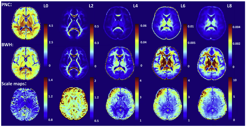
where l is the order of the RISH feature and ε is a small non-zero constant. Fig. 3 shows five mean templates of RISH features for l = {0, 2, 4, 6, 8} from left to right for PNC (top row) and BWH (middle row) sites. Note that, each RISH feature captures different frequencies of the dMRI signal. For instance, RISH feature for l = 0 captures isotropic components of the diffusion signal, while l = 2 is similar to FA and l ≥ 4 captures higher order frequencies. Consequently, RISH feature for each l represents different microstructural tissue properties of the dMRI signal, which can be modified to harmonize the dMRI data from different sites without changing the underlying fiber orientations and hence the fiber connectivity of the subjects. Note the sharp differences in the RISH feature maps between the two sites, indicating regional and tissue specific non-linear differences between the sites. Fig. 3 also shows the scale maps learned for each RISH feature from the training subjects at both sites. As expected, the difference between sites is region and tissue specific.

Fig. 3.

RISH Features for SH orders of l = {0, 2, 4, 6, 8} are depicted in each sub-figure from left to right for PNC site (top row) and BWH site (middle row). Scale maps for each RISH feature show the between-site mapping obtained between controls from two sites (bottom row).

2.3.4. Harmonization

We apply the linear map (for each RISH feature separately) learned from the training data set to all new subjects in the target site by non-rigid spatial transformation of the linear maps to the native subject space. The non-rigid transformation is obtained by registering the RISH features of each subject to the template space. The inverse of this transformation is applied to the estimated inter-site linear map. The harmonized dMRI signal is then calculated by scaling the SH coefficients of the signal at each voxel in the subject space as follows:

$${\widehat{C}}_{lm}\left(x\right)={\widehat{\mathcal{G}}}_l\left(x\right)C_{lm}\left(x\right)$$ (3)

where ${\widehat{\mathcal{G}}}_l\left(x\right)$ is the scale map in the subject space and ${\widehat{C}}_{lm}\left(x\right)$ the scaled SH coefficients. The final diffusion signal is then computed using:

$$\widehat{S}\left(x\right)={\displaystyle \sum }_l{\displaystyle \sum }_m{\widehat{C}}_{lm}\left(x\right)Y_{lm}$$ (4)

2.4. Training set size

In this section we investigate the effect of the size of training subjects on the estimated inter-site RISH feature map. We begin by selecting a matched set of subjects at both sites (PNC and BWH) varying in size from 2 to 25 (consecutive even numbers). For each training set size, we iteratively generated a bootstrap sample and checked whether the subjects matched between the sites using an unpaired t-test. Unmatched samples were discarded until we obtained 100 matched bootstrap samples. The subjects were matched across sites for age, gender and IQ.

To further verify our method, we also used an independent site (Oxford) with 32 healthy young adolescent subjects that were matched with the PNC dataset (See Fig. 4(b)). The same experiment was repeated, where an inter-site mapping was learnt with 100 bootstrap samples (well-matched subjects as described earlier).

Fig. 4.

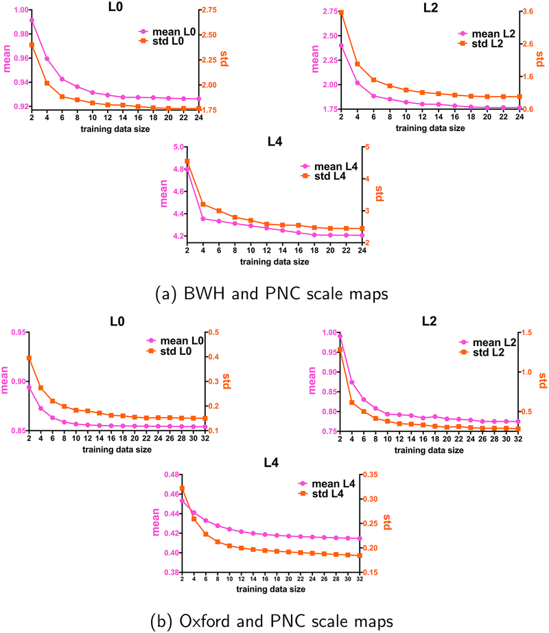
Training size of subjects from (a) PNC and BWH sites (2–24 subjects) and (b) PNC and Oxford (2–32 subjects) plotted as a function of mean (pink) and standard deviation (std) (orange) of scale maps for RISH features of L0 (top-left), L2 (top-right) and L4 (bottom) to decide how many training subjects are needed to learn the scanner differences across sites. We see that at-least 16 subjects are needed for training in both the datasets.

To demonstrate the effect of training data size, in Fig. 4, we plot the number of training subjects versus the estimated whole brain mean and standard deviation (std) of the scale map. Our goal is to determine the minimum number of training subjects after which the mean and standard deviation of the scale maps do not change significantly, i.e. adding more subjects to the training data does not affect the scale maps. In Fig. 4(a) we show the mean and standard deviation curves for RISH features for order 0, 2 and 4 (order 6 and 8 behave very similar to order 4), for the PNC-BWH sites. We observe that the curves become almost stable after a training size of 16, which implies that at-least 16 well matched subjects at each site are needed to learn a robust mapping between sites for dMRI data harmonization. Further, we also observe that the average difference of the mean and std between training size of 18 and 20 is ≤ 0.01.

Similarly, for the PNC-Oxford sites (Fig. 4(b)), the change in the estimated scale maps for all the RISH features hardly changes once at-least 16 matched subjects from each site are used. Consequently, in the rest of this work, we set our training data set size to 20 which can provide robust learning of scanner differences between sites.

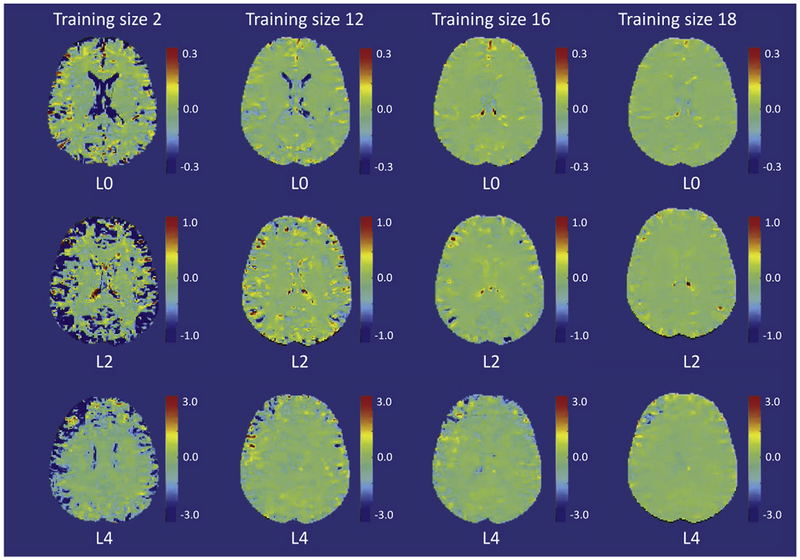
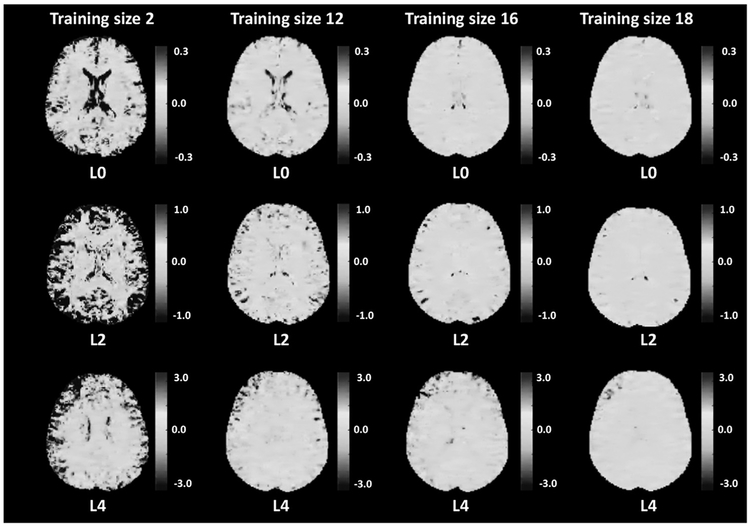
To provide a more region-specific view, in Fig. 5, we depict the differences between the scale maps (PNC-BWH) with a training size of 20 (as “gold standard”) and some representative training data sets of size 2, 12, 16 and 18 for each RISH feature (L0, L2 and L4). Even though we observe large differences between the data sets with 20 subjects and 2 subjects, we see that the voxel-wise differences significantly decrease and the difference maps become more similar after a training size of 16. A gray-scale image of the same figure is included in the Appendix.

Fig. 5.

Voxel-wise scale map differences between RISH feature scale map (L0, L2 and L4) estimated with a training size of 20 (as “gold standard”) and some representative training data size of 2, 12, 16 and 18 shown in each column respectively. The grayscale figure is also provided in the appendix: Figure A1.

3. Experiments and results

3.1. Experimental setup

In this section, we describe experiments to evaluate the performance of the proposed algorithm. First, to show that the harmonization works equally well irrespective of the choice of the reference site, we will evaluate the performance of our method using two experiments. In the first experiment, we choose BWH as the reference site and PNC as the target site, whereas in the second experiment we use PNC as the reference site and BWH as the target site. Another aim of these experiments is also to demonstrate the robustness of the proposed technique to preserve group differences despite the size of the test data sets. For example, we evaluate age-related group differences in the PNC data which has a large number of subjects, as well as the BWH site which has a small sample size.

We use dMRI-derived measures of FA, MD and generalized-FA (GFA), which are typically used in neuroimaging studies to understand the effect of harmonization. These measures were also chosen as they are known to change with age in a nonlinear fashion (Yeatman et al., 2014; Lebel et al., 2008) and show different maturational pattern between males and females (Gur et al., 1999; Asato et al., 2010). Hence, our experiments consisted of evaluating the effect sizes between three/two groups (separated by age or sex) before and after harmonization. To investigate performance of the harmonization in different regions of the brain that are known to mature at different speeds and are sex dependent, we used the Illinois Institute of Technology (IIT) Human Brain Atlas (Varentsova et al., 2014; Zhang and Arfanakis, 2018). We used 16 different white matter bundles¹ from this atlas to evaluate the performance of our method. We set a threshold to 0.2 for all subjects to clearly define the regions-of-interest (ROIs) in the IIT probabilistic atlas. Mean FA, MD and GFA were computed in each region for all subjects before and after harmonization to use in the upcoming experiments.

In Section 3.2.1, we test the learning (mapping) capabilities and performance of our algorithm on 20 training subjects selected from each site. In Section 3.2.2, we show how the aging and gender effects are preserved after harmonization in a large number of test subjects. In Section 3.2.3, we demonstrate that the proposed harmonization procedure preserves fiber orientation by comparing fiber bundle tracing results before and after harmonization.

3.2. Results

3.2.1. Evaluation on training subjects

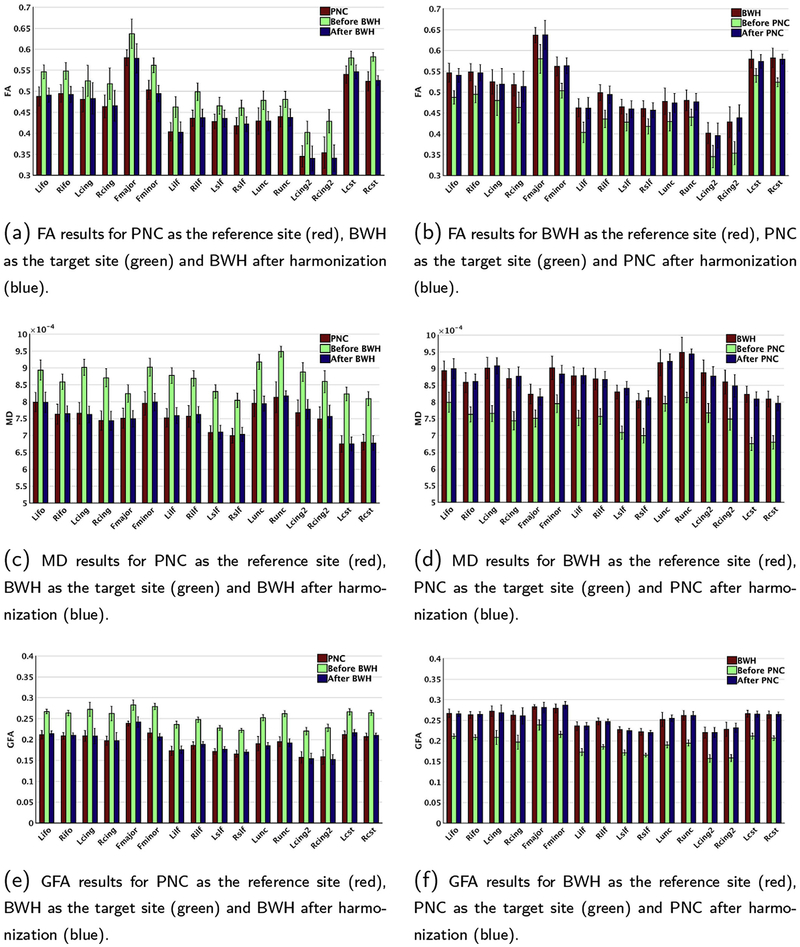
In Fig. 6, we show the mean FA (a, b), mean MD (c, d) and mean GFA (e, f) values in the reference site (red), the target site (green) and the harmonized results (blue) for each of the major white matter bundles (from the IIT atlas) on the training data. In (a, c, e), respectively, we depict the results for FA, MD and GFA with PNC as the reference site and BWH as the target site. In (b, d, f), the experiment is repeated with BWH as the reference site and PNC as the target site. We also observe that the site differences are not uniform but vary in a highly nonlinear fashion across the brain and for all measures. We note that the site differences appear to be more for MD as compared to FA and GFA, which was also reported in (Vollmar et al., 2010).

Fig. 6.

Comparison of diffusion measures (FA, MD and GFA) across sites: red: reference site, green: target site, and blue: after harmonization of target to reference. Left column: PNC is selected as reference site and BWH is selected as target site. Right column: BWH is selected as reference site and PNC is selected as target site. In both scenarios, large statistical differences are observed prior to harmonization which are removed after harmonization.

To statistically analyze each diffusion measure before and after harmonization, the parametric paired t-test was applied to all major bundles between two sites: (i) reference site and target site (before harmonization); (ii) reference site and harmonized site (after harmonization). See Table 5 for the statistics of PNC as the target site and see Table 6 for the statistics of BWH as the target site. We observe a significant difference between the two sites for all measures (p < 1e − 4 for all bundles and measures) before harmonization. After harmonization, the statistical difference between controls from both sites is removed for all bundles and measures.

Table 5.

The statistics for PNC data: paired t-test was applied to each diffusion measure of all major bundles between two sites: (i) BWH as the reference site and PNC as the target site (the statistics are reported in before PNC rows); (ii) BWH as the reference site and harmonized PNC results (the statistics are reported in after PNC rows).

Data	P value	t, df	Mean of	SD of	95%	R2	r
			differences	differences	CI
Before PNC: FA	<0.0001	t = 18.14 df = 15	−0.04869	0.01074	−0.05442 to −0.04297	0.9564	0.9861
Before PNC: MD	<0.0001	t = 24.89 df = 15	− 1.165e-4	1.871e-4	−1.264e-4 to 1.065e-4	0.9764	0.8981
Before PNC: GFA	<0.0001	t = 37.59 df = 15	−0.05979	0.006362	−0.06318 to −0.0564	0.9895	0.9659
After PNC: FA	0.1825	t = 1.398 df = 15	−0.001756	0.005025	−0.004434 to 0.0009215	0.1153	0.9968
After PNC: MD	0.1661	t = 1.456 df = 15	−2.708e-6	7.442e-6	−6.674e-6 to 1.257e-6	0.1238	0.9838
After PNC: GFA	0.7964	t = 0.2626 df = 15	0.0001812	0.002761	−0.00129 to 0.001652	0.004576	0.9913

CI: confidence interval; r: correlation coefficient (to observe how effective the pairing is); R²: partial eta squared (to observe how big the difference is).

Table 6.

The statistics for BWH data: paired t-test is applied to each diffusion measure of all major bundles between two sites: (i) PNC as the reference site and BWH as the target site (the statistics are reported in before BWH rows); (ii) PNC as the reference site and harmonized BWH results (the statistics are reported in after BWH rows).

Data	P value	t, df	Mean of	SD of	95%	R2	r
			differences	differences	CI
Before BWH: FA	<0.0001	t = 18.77 df = 15	0.05251	0.01119	0.04655 to 0.05847	0.9591	0.9887
Before BWH: MD	<0.0001	t = 24.89 df = 15	1.165e-4	1.871e-5	1.065e-4 to 1.264e-4	0.9764	0.8981
Before BWH: GFA	<0.0001	t = 37.59 df = 15	0.05982	0.006364	0.05642 to 0.06321	0.9895	0.9658
After BWH: FA	0.8119	t = 0.2423 df = 15	−0.00075	0.01238	−0.007348 to 0.005848	0.003898	0.9885
After BWH: MD	0.9235	t = 0.09761 df = 15	2.956e-07	1.211e-5	−6.159e-006 to 6.751e-006	6.348e-4	0.9629
After BWH: GFA	0.7913	t = 0.2694 df = 15	0.0002844	0.004222	−0.001965 to 0.002534	0.004815	0.9847

CI: confidence interval; r: correlation coefficient (to observe how effective the pairing is); R²: partial eta squared (to observe how big the difference is); ns: not-significant.

3.2.2. Effect size comparison in test subjects

Once a mapping between the sites is estimated from the 20 training subjects (per site), it is applied to the rest of the data set from the target site (i.e., data from all subjects of the target site are updated or harmonized). Any harmonization technique should preserve the inter-subject biological variability and group differences at each site, while only removing scanner related effects. This can be tested by ensuring that the effect sizes between groups is maintained before and after harmonization. White matter maturation (as measured by FA) with age has been well-documented in the literature (Lebel et al., 2008), along with the differential trajectory of this maturation between males and females (Gur et al., 1999). We use this as a test-bed to demonstrate that the effect sizes between groups before and after harmonization is maintained. Specifically, we calculate the effect sizes between groups categorized by age and sex as described in Table 4.

Table 4.

Three age groups in BWH and PNC data for females and males separately.

Gender	Group	BWH	PNC
Female	1st	14–22 years (n = 8)	8–12 years (n = 97)
	2nd	23–33 years (n = 9)	13–17 years (n = 186)
	3rd	38–48 years (n = 5)	18–22 years (n = 127)
Male	1st	14–24 years (n = 25)	8–12 years (n = 90)
	2nd	24–38 years (n = 7)	13–17 years (n = 183)
	3rd	42–54 years (n = 16)	18–22 years (n = 107)

Abbreviations: Dataset: PNC - Philadelphia Neurodevelopmental Cohort; BWH - Brigham and Women’s Hospital; F: females; M: males.

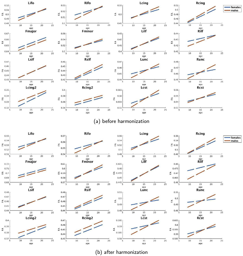
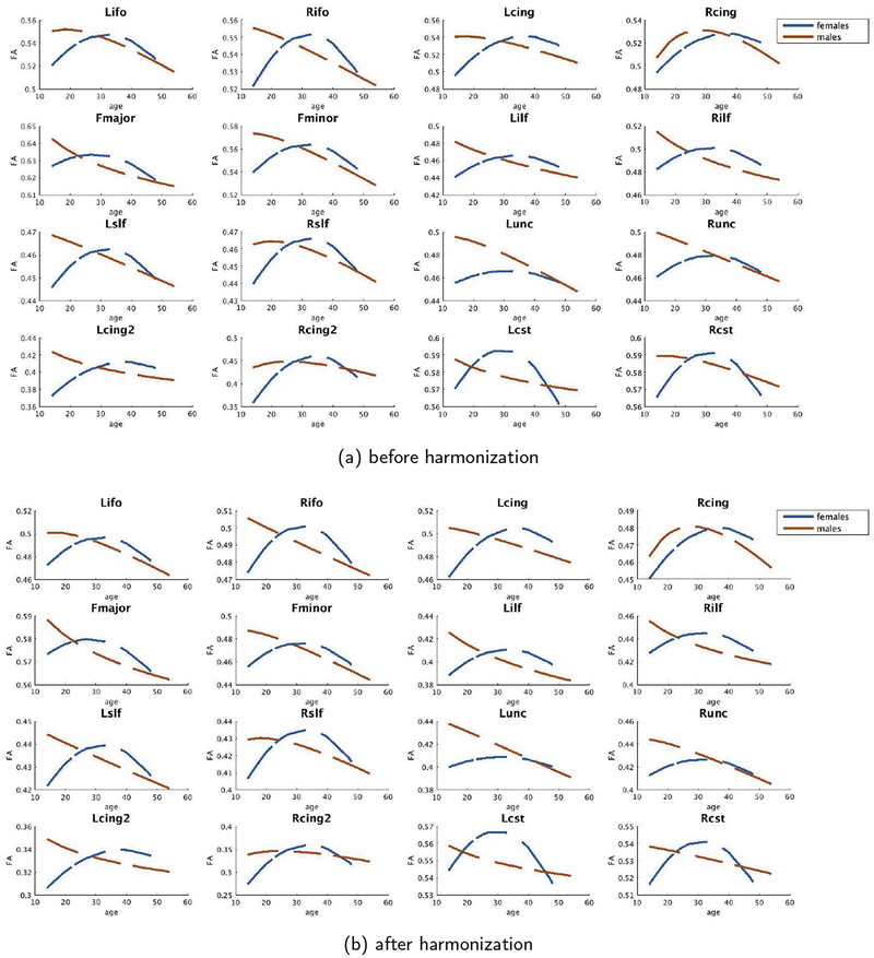
In our first experiment, we calculate the group differences between males and females in FA for each of the three age groups (i.e., matched for age). Our goal is to test if the effect sizes observed in the original test data are preserved after harmonization to a target site. In our second experiment, we calculate the effect sizes due to age before and after harmonization. For both of the experiments, we set: (1) BWH as the reference site and PNC as the target site (see Figure Appendix B.2(a) to see the maturation curves in PNC data); (2) PNC as the reference site and BWH as the target site (see Figure Appendix B.3(a) to see the maturation curves in BWH data).

3.2.2.1. Sex differences (effect sizes) before and after harmonization.

We compute the effect sizes using Cohen’s d between females and males matched for age for each of the three age groups from Table 4. Mathematically, Cohen’s d can be written as: $d=\frac{M_{fi}-M_{mi}}{S_{pooled}}$ where M is the mean FA of the i^th group, f represents females, m represents males. S_pooled is given by $S_{pooled}=\sqrt{\frac{\left(n_{fi}-1\right)S_{fi}^2+\left(n_{mi}-1\right)S_{mi}^2}{n_{fi}+n_{mi}-2}}$ where n is the number of subjects and S_mi, S_fi are the standard deviations for the male and female groups respectively.

3.2.2.1.1. BWH reference site.

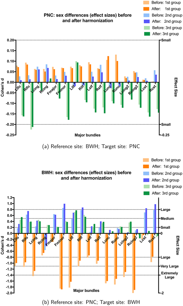
In Fig. 7(a), we show plots for white matter bundles before and after harmonization. Here BWH is the reference site and PNC is the target site. As can be seen, the effect sizes between the sexes before and after harmonization are almost the same for all age groups, that is, if the effect sizes are small before harmonization, they stay small after harmonization as well. Similar observations can be made for medium and large effect sizes. We however note that, in general, the effect sizes after harmonization are slightly lower than the original, potentially because of some smoothing effects that occur due to interpolation. Nevertheless, these differences are minor and do not change the outcome of statistical analysis.

Fig. 7.

The effect sizes (Cohen’s d) between the sexes for all age groups before and after harmonization. Note that the effect sizes are maintained by the harmonization procedure.

In Table 1, we provide quantitative values for the effect sizes between groups for BWH as the reference site and PNC as the target site for each major bundle before and after harmonization. We also report the absolute differences (Δ) between the effect sizes before and after harmonization. Also reported are results when the effect sizes are grouped into small (d~0.2), medium (d~0.5), large (d~0.8), very large (d~1.1) and extremely large (d~1.4) effect sizes. We report the average absolute differences in the effect sizes in each group (Table 7-cyan rows). As can be seen, the effect sizes are preserved after harmonization (i.e., absolute differences in effect sizes before and after harmonization are always close to the original with the average difference being 0.0132).

Table 7.

Grouped (from small to extremely large) average sex differences in terms of effect sizes before and after harmonization. Cyan rows: the results for BWH as reference and PNC as the target site; Gray rows: the results for PNC as reference and BWH as the target site. Δ is the absolute difference between effect sizes (before and after harmonization); - implies none of the fiber bundles demonstrated those effect sizes.3

	Small	Medium	Large	Very Large	Extremely Large
Before PNC	0.068	0.224	−	−	−
After PNC	0.066	0.212	−	−	−
Δ PNC	0.002	0.012	−	−	−
Before BWH	0.102	0.336	0.686	0.947	1.584
After BWH	0.154	0.379	0.720	0.884	1.440
Δ BWH	0.052	0.043	0.034	0.063	0.144

3.2.2.1.2. PNC reference site.

We also perform a similar analysis for PNC as the reference site and BWH as the target site. At the BWH site, the number of female subjects is very small. Despite this small sample size, the harmonization algorithm preserves the maturation trends very accurately (i.e., trends are very similar to that before harmonization), demonstrating the robustness of the proposed method. However, as seen in Fig. 7(b), (and Figure Appendix B.3), small sample sizes can provide misleading (and potentially inaccurate) results as has been shown by several works in the literature. Here, we show these results only to demonstrate that the inter-subject biological variability is preserved by our harmonization algorithm despite the small sample size (test samples) used. We note that no other inferences about sexual dimorphisms can be made from these results from the BWH site.

In Table C1, we provide quantitative values for the effect sizes for BWH samples before and after harmonization, and their absolute differences for each major bundle. Due to smaller data size of the females and a totally different age range of females and males in each group, unlike the previous experiment, we also observe medium, large, very large and extremely large effect sizes prior to harmonization which are preserved after harmonization (Δ is always < 0.2). Grouping the fiber bundles based on their effect sizes, we once again observe that the effect sizes are preserved after harmonization (Table 7-gray rows), i.e., effect sizes that were small, medium, or large stay small, medium and large respectively after harmonization.

3.2.2.2. Age related effect sizes before and after harmonization.

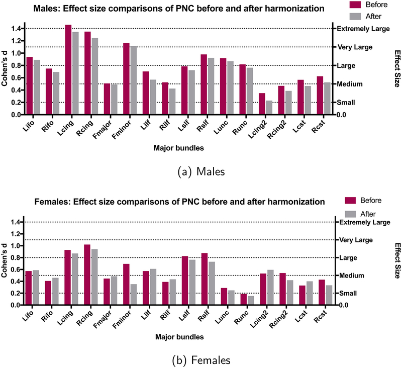
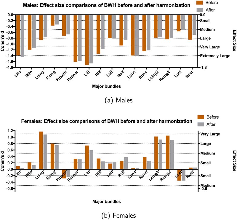
In this experiment, our aim is to show that the effect sizes due to aging are preserved after harmonization. For this purpose, we compute the effect sizes (Cohen’s d) between the first and the third age group from Table 4 for both males and females separately. Cohen’s d is calculated in a similar fashion as above.

3.2.2.2.1. BWH reference site.

In this case, BWH is the reference site and all data analysis before and after harmonization is done on the PNC site. Since FA increases in young adolescent subjects during maturation (Lebel et al., 2008), it is natural to observe mostly large and positive effect sizes due to aging. Besides, the effect sizes are highly sensitive to gender (see Fig. 8). As can be seen, the effect sizes stay almost the same after harmonization in all experiments. In Table C3, we report the effect sizes of the first and the third age group before and after harmonization and their absolute differences Δ for males and females separately. Group differences as measured by effect sizes, which are significantly different before harmonization for all bundles, still stay significantly different after harmonization (Δ is always < 0.2). Additionally, the grouped effect size results stay similar after harmonization (Table 8-cyan rows).

Fig. 8.

Results for age-related differences between groups with BWH as the reference site and PNC as the target site. The effect sizes (Cohen’s d) between the first and the last group (see Table 4 for the age distribution of the groups) are shown for each gender separately (before harmonization (purple) and after harmonization (gray)).

Table 8.

Comparison of the average grouped (from small to extremely large) aging effect sizes before and after harmonization. Cyan rows: the results for BWH is reference and PNC is the target site; Gray rows: the results for PNC is reference and BWH is the target site. Δ is the absolute difference between effect sizes (before and after harmonization).4

	Small	Medium	Large	Very Large	Extremely Large
Before PNC	0.188	0.389	0.615	0.913	1.324
After PNC	0.153	0.372	0.538	0.844	1.235
Δ PNC	0.035	0.017	0.077	0.069	0.089
Before BWH	0.092	0.315	0.722	0.924	1.381
After BWH	0.090	0.283	0.660	0.822	1.338
Δ BWH	0.002	0.032	0.062	0.102	0.043

In this regard, we would also like to point the results of age-dependent maturation curves in the PNC data set. As can be seen in Figure B2, the maturation curves are accurately preserved by the harmonization algorithm. When PNC data is the target site (i.e., PNC data is updated for harmonization), we see a robust trend in maturation of different white matter bundles consistent with those reported in the literature (Paus et al., 2001; Paus, 2010).

3.2.2.2.2. PNC reference site.

We also perform a similar analysis for PNC as the reference site and BWH as the target site (i.e., BWH data was harmonized and analyzed before and after harmonization). Due to small sample size and differences in age-ranges, the maturation curves and the effect sizes do not match with those from the much larger PNC data set. However, to clarify once more, our aim is only to validate the harmonization performance regardless of the underlying trends in the data. As can be seen, the harmonization procedure preserves the trends as well as the effect sizes. In Table C4, we report the effect sizes and Δ for the BWH site before and after harmonization for males and females respectively. The effect sizes are preserved after harmonization for all white matter bundles (see also Fig. 9) and for each group (Table 8-gray rows).

Fig. 9.

Results for age-related differences between groups with PNC as the reference site and BWH as the target site. The effect sizes (Cohen’s d) between the first and the last group (see Table 4 for the age distribution of the groups) are shown for each gender separately (before harmonization (orange) and after harmonization (gray)).

3.2.3. Tractography analysis

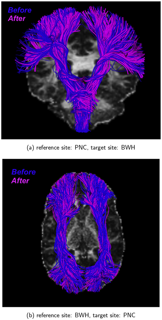
In order to ensure that our harmonization method (which involves modifying the dMRI signal) does not in any way to change the fiber orientations, we performed whole brain tractography using a multitensor unscented Kalman filter (UKF) method (Malcolm et al., 2010; Reddy and Rathi, 2016). The same parameters were used to generate whole brain tracts from the original and harmonized dMRI data. Next, the White Matter Query Language was utilized (WMQL) (Wassermann et al., 2016) to extract specific anatomical white matter bundles from the whole brain tracts. Fig. 10 depicts WMQL results for corticospinal tract (CST) and the inferior occipital-frontal fibers (IOFF) before (blue) and after (pink) harmonization. After extracting the tracts from a subject before and after harmonization, the Bhattacharyya overlap distance (B) was used to quantify the overlap between the tracts (Rathi et al., 2013):

$$B=\frac{1}{3}\left(\int \sqrt{P_h\left(x\right)P\left(x\right)}dx+\int \sqrt{P_h\left(y\right)P\left(y\right)}dy+\int \sqrt{P_h\left(z\right)P\left(z\right)}dz\right)$$ (5)

where P(.) represents the ground truth spatial probability distribution of the fiber bundle, P_h(.) is the spatial probability distribution of the tracts from the harmonized data and $\left(x,y,z\right)\in {ℝ}^3$ are the fiber coordinates. B is 1 for a perfect match between two fiber bundles and 0 for no overlap at all. We observed very high overlap greater than 0.93 for all fiber bundles indicating that fiber orientation is well preserved by the harmonization algorithm.

Fig. 10.

Significant (> 93%) overlap is seen in CST and IOFF fiber bundles before and after harmonization. Blue: before harmonization; Pink: after harmonization.

3.3. Comparison of our method with ComBat data pooling technique

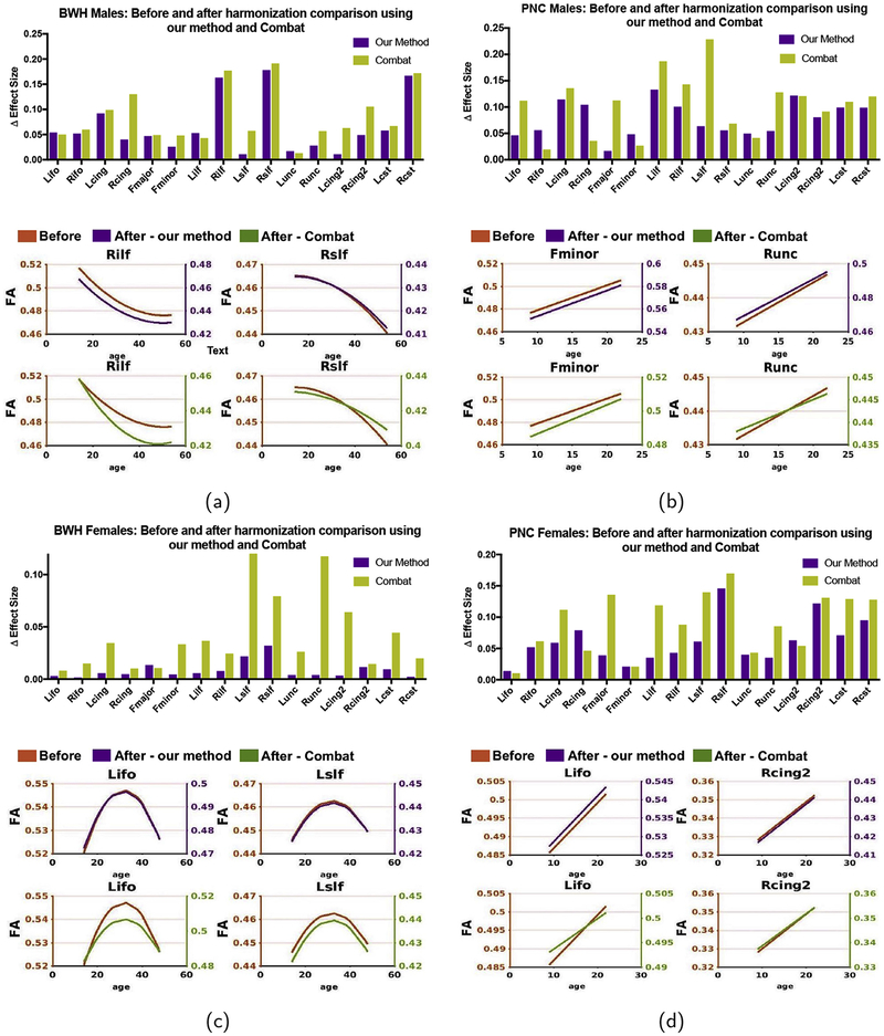
To validate the performance of our harmonization algorithm, we compare our method with the recently proposed ComBat statistical harmonization tool² using both PNC and BWH (870 subjects in total). We include age and gender as biological covariates for all results. In the first experiment, we choose PNC as the reference site and BWH as the target site (Fig. 11 (a: for males, c: for females)), whereas in the second experiment we use BWH as the reference site and PNC as the target site (Fig. 11 (b: for males, d: for females)). We investigate the maturational pattern of WM ROIs using FA as described in section 3.2.2.2. Our aim is to see if the effect sizes due to aging are preserved after harmonization. In each subfigure, we plot Δ- the effect size difference before and after harmonization on the top and the maturation curves of a few representative tracts on the bottom. As can be seen, for both harmonization methods Δ is always < 0.2, however, the proposed method outperforms ComBat in many WM regions (see effect sizes in Fig. 11(c)). We also notice that ComBat has slightly higher error as measured by Δ (~ 0.23) for PNC males in the Lslf region apart from the fact that several maturational curves do not retain the same shape after harmonization (see curves for BWH: Females - Lilf, or BWH: Males: Rilf). For the majority of the tracts, we observe that our harmonization method performs better than ComBat.

Fig. 11.

Comparison of our harmonization method with the ComBat data pooling technique: Δ is the absolute differences of the effect sizes before and after harmonization for each method. Also shown are maturational curves before and after harmonization using each of the methods. As can be seen, ComBat fails to accurately preserve the maturational curves in Rilf and Lifo, whereas those are preserved using the proposed technique.

4. Discussion

We believe that accurate harmonization of dMRI data is of utmost importance to allow for a large-scale data-driven way to understand brain disorders. In this paper, we presented a harmonization method to retrospectively remove scanner-specific differences from the raw dMRI signal across various sites, even if acquired with different acquisition parameters. The harmonization procedure requires a well-matched set of controls across sites to learn the mapping between sites.

Acquisition parameters, magnetic field inhomogeneities, coil sensitivity, and other scanner related effects can cause non-linear changes in the signal in different tissue types. To remove these site effects, we first mapped the b-values from each site to a canonical b-value of 1000s/mm² and resampled the data to 1.5³ mm³ (Section 2.3.1). Later, we utilized RISH features that are able to capture different frequency components of the diffusion signal to learn the inter-site differences (Section 2.3.2). In Fig. 3, we showed that the scanner related differences are substantially different for sub-cortical gray, versus the neighboring white matter region or the distant cortical gray matter regions. Further, these differences can be captured selectively by the different frequency bands of the SH basis (i.e., in different RISH features).

We note that, the methodology proposed here harmonizes the raw dMRI signal in a model-independent manner. Further, dMRI data harmonization has to be done only once. Thus, any subsequent analysis will necessarily be consistent, unlike methods (such as ComBat) that work with model-specific measures such as FA, which are obtained at the last stage of the processing pipeline. Note that, it is not clear how nonlinear scanner effects affect the downstream processing and model fitting of dMRI data. Consequently, we recommend that dMRI data be harmonized at the earliest possible processing stage. In the interest of open-science, we will make the code publicly available soon.

Using several experiments, in this paper, we evaluated our method’s performance on two independent sites: PNC with 800 healthy controls and BWH with 70 healthy controls. Our results lead us to conclude the following: (i) At-least 16 to 18 well matched healthy controls from each site are required to learn a robust mapping that can capture only site-related differences. (ii) Irrespective of the effect size (small, medium or large), the proposed harmonization procedure preserved the effect sizes after harmonization. (iii) The harmonization procedure also ensured that the fiber orientation directions were left unchanged, which is important for brain connectivity analysis.

5. Limitations

Despite its ability to harmonize clinical dMRI data, the proposed method nevertheless has certain limitations. First, the b-value matching procedure described herein works only in the lower b-value regime (500 < b < 1500). Beyond this range, a non-linear technique such as the one in Rathi et al. (2014) would have to be used for adjusting the b-values across sites. Note that, this limitation is not specific to our technique, and is also a limitation of other techniques such as ComBat. Interpolation to normalize the spatial resolution might result in some smoothing of the data, which is potentially the reason for the slight differences in effect sizes seen in our experiments. Similar smoothing effects can also be expected in the case of ComBat (which requires matching of spatial resolution). Due to scanner drift during the length of a longer neuroimaging study, it is necessary to use control subjects spread during the entire duration of the study. In this case, ComBat has an advantage as it does not need matched control subjects. However, for proper use of ComBat, nonlinearities due to age and sex differences have to be accurately modeled to capture effects of demographic and other variables (which may not be known accurately if the sample size is small). We also note that, signal-to-noise ratio of the raw dMRI data from each site may also play a role in our ability to accurately harmonize multi-site data. While the robustness of the harmonization technique for a range of SNR values was demonstrated using simulation data in Mirzaalian et al. (2016), yet this needs to be tested using in-vivo data.

Despite these limitations, we believe that the proposed method is the only technique currently available that can directly harmonize the raw dMRI signal. None of the previous approaches including ComBat can reconstruct the raw harmonized signal, which is essential for consistent microstructural, tractography and connectivity studies.

Appendix A

Figure A.1.

Grayscale figure of Fig. 5: Voxel-wise scale map differences between RISH feature scale map (L0, L2 and L4) estimated with a training size of 20 (as “gold standard”) and some representative training data size of 2, 12, 16 and 18 shown in each column respectively.

Appendix B. Age-related trends in FA, before and after harmonization

Figure B.2.

Reference Site: BWH, before and after harmonization female (blue) and male (orange) age vs FA curves of PNC for each major white matter bundle.1

Figure B.3.

Reference Site: PNC, before and after harmonization female (blue) and male (orange) age vs FA curves of BWH for each major white matter bundle.

Appendix C. Effect sizes before and after harmonization for BWH as the reference site and PNC as the target site

C.1. Analysis of sex differences

Table C.1.

Target site: PNC. Sexual dimorphism effect sizes effect sizes before and after harmonization for each major bundle. Absolute differences (Δ) between before and after harmonization effect sizes are observed to be < 0.2 in all cases.

WM ROIs	Age 8–12			Age 13–17			Age 18–22
	Before	After	Δ	Before	After	Δ	Before	After	Δ
Lifo	0.079	0.072	0.007	0.028	0.010	0.018	−0.157	−0.162	0.005
Rifo	0.093	0.084	0.009	0.033	0.014	0.019	−0.224	−0.212	0.012
Lcing	0.063	0.059	0.004	0.074	0.061	0.013	−0.027	−0.040	0.013
Rcing	0.063	0.051	0.012	0.085	0.068	0.017	0.006	0.018	0.012
Fmajor	0.073	0.062	0.011	0.032	0.015	0.017	−0.053	−0.077	0.024
Fminor	0.069	0.067	0.002	0.049	0.031	0.018	−0.165	−0.178	0.013
Lilf	0.074	0.067	0.007	−0.002	−0.019	0.017	0.100	0.094	0.006
Rilf	0.081	0.075	0.006	0.002	−0.015	0.017	−0.084	−0.095	0.011
Lslf	0.095	0.085	0.010	0.050	0.027	0.023	−0.125	−0.143	0.018
Rslf	0.066	0.063	0.003	0.083	0.047	0.036	−0.119	−0.147	0.028
Lunc	0.106	0.124	0.018	−0.019	−0.028	0.009	−0.090	−0.100	0.010
Runc	0.131	0.101	0.030	−0.012	−0.020	0.008	−0.107	−0.121	0.014
Lcing2	0.028	0.020	0.008	0.026	0.008	0.018	−0.062	−0.082	0.020
Rcing2	0.053	0.046	0.007	0.047	0.025	0.022	−0.106	−0.121	0.015
Lcst	0.012	0.011	0.001	0.019	0.007	0.012	−0.143	−0.163	0.020
Rcst	−0.001	0.002	0.003	0.057	0.036	0.021	−0.127	−0.144	0.017

Table C.2.

Target site: BWH. Sexual dimorphism effect sizes before and after harmonization for each major bundle. Absolute differences (Δ) between before and after harmonization effect sizes are observed to be < 0.2 in all cases.

WM ROIs	Age 8–12			Age 13–17			Age 18–22
	Before	After	Δ	Before	After	Δ	Before	After	Δ
Lifo	−1.089	−0.995	0.094	0.172	0.315	0.143	0.455	0.546	0.091
Rifo	−1.125	−0.968	0.157	0.629	0.749	0.120	0.388	0.394	0.006
Lcing	−1.431	−1.260	0.171	0.234	0.426	0.192	0.450	0.404	0.046
Rcing	−0.736	−0.655	0.081	−0.560	−0.429	0.131	0.281	0.278	0.003
Fmajor	−0.288	−0.281	0.007	0.645	0.625	0.020	0.224	0.214	0.010
Fminor	−1.851	−1.878	0.027	0.853	0.993	0.140	0.413	0.384	0.029
Lilf	−1.818	−1.622	0.196	0.497	0.694	0.197	0.717	0.774	0.057
Rilf	−1.104	−0.915	0.189	0.780	0.868	0.088	0.619	0.557	0.062
Lslf	−0.814	−0.738	0.076	0.055	0.237	0.182	0.203	0.315	0.112
Rslf	−1.018	−0.915	0.103	0.195	0.392	0.197	0.338	0.386	0.048
Lunc	−1.675	−1.599	0.076	−0.059	0.115	0.174	−0.008	0.070	0.078
Runc	−1.714	−1.524	0.190	0.178	0.142	0.036	0.232	0.217	0.015
Lcing2	−1.462	−1.294	0.168	−0.027	0.037	0.064	0.364	0.393	0.029
Rcing2	−2.073	−1.896	0.177	0.100	0.141	0.041	−0.051	−0.164	0.113
Lcst	−0.199	−0.059	0.140	0.703	0.842	0.139	−0.058	0.082	0.140
Rcst	−0.962	−0.781	0.181	0.784	0.979	0.195	−0.124	−0.080	0.044

Appendix C.2. Analysis of aging

Table C.3.

Target site: PNC. Age related effect sizes before and after harmonization for each major bundle. Absolute differences (Δ) between before and after harmonization effect sizes are observed to be < 0.2 in all cases.

WM ROIs	Males			Females
	Before	After	Δ	Before	After	Δ
Lifo	0.938	0.891	0.046	0.574	0.588	0.014
Rifo	0.749	0.693	0.056	0.407	0.459	0.052
Lcing	1.459	1.345	0.114	0.929	0.870	0.059
Rcing	1.349	1.245	0.104	1.021	0.942	0.079
Fmajor	0.508	0.491	0.017	0.447	0.486	0.039
Fminor	1.162	1.114	0.048	0.694	0.353	0.341
Lilf	0.703	0.570	0.133	0.575	0.610	0.035
Rilf	0.526	0.425	0.101	0.391	0.434	0.043
Lslf	0.785	0.722	0.064	0.825	0.764	0.061
Lunc	0.918	0.868	0.050	0.288	0.248	0.040
Runc	0.818	0.763	0.054	0.188	0.153	0.035
Lcing2	0.351	0.229	0.122	0.532	0.595	0.063
Rcing2	0.468	0.387	0.080	0.541	0.419	0.122
Lcst	0.566	0.467	0.099	0.329	0.400	0.071
Rcst	0.625	0.526	0.099	0.428	0.333	0.095

Table C.4.

Target site: BWH. Age related effect sizes before and after harmonization for each major bundle. Absolute differences (Δ) between before and after harmonization effect sizes are observed to be < 0.2 in all cases.

WM ROIs	Males			Females
	Before	After	Δ	Before	After	Δ
Lifo	−1.389	−1.443	0.054	0.096	0.036	0.060
Rifo	−1.195	−1.143	0.052	0.219	0.135	0.084
Lcing	−0.861	−0.769	0.092	1.174	1.084	0.090
Rcing	−0.372	−0.332	0.040	0.800	0.750	0.050
Fmajor	−0.719	−0.672	0.047	−0.280	−0.241	0.039
Fminor	−1.606	−1.580	0.026	0.326	0.312	0.014
Lilf	−1.714	−1.661	0.053	0.739	0.595	0.144
Rilf	−1.333	−1.170	0.163	0.336	0.246	0.090
Lslf	−0.801	−0.812	0.011	0.180	0.234	0.054
Rslf	−1.050	−0.872	0.178	0.258	0.381	0.123
Lunc	−1.391	−1.408	0.017	0.039	0.035	0.004
Runc	−1.244	−1.216	0.028	0.378	0.266	0.112
Lcing2	−0.783	−0.772	0.011	1.019	0.926	0.093
Rcing2	−0.838	−0.789	0.049	1.047	0.903	0.144
Lcst	−0.567	−0.509	0.058	−0.352	−0.351	0.001
Rcst	−0.852	−0.685	0.167	0.052	0.054	0.002

References

- Asato M, Terwilliger R, Woo J, Luna B, 2010. White matter development in adolescence: a dti study. Cerebr. Cortex 20, 2122–2131. [DOI] [PMC free article] [PubMed] [Google Scholar]
- Avants BB, Tustison NJ, Song G, Cook PA, Klein A, Gee JC, 2011. A reproducible evaluation of ants similarity metric performance in brain image registration. Neuroimage 54, 2033–2044. http://dblp.uni-trier.de/db/journals/neuroimage/neuroimage54.html#AvantsTSCKG11. [DOI] [PMC free article] [PubMed] [Google Scholar]
- Avants BB, Yushkevich P, Pluta J, Minkoff D, Korczykowski M, Detre J, Gee JC, 2010. The optimal template effect in hippocampus studies of diseased populations. Neuroimage 49, 2457–2466. http://www.sciencedirect.com/science/article/pii/S1053811909010611. 10.1016/j.neuroimage.2009.09.062. [DOI] [PMC free article] [PubMed] [Google Scholar]
- Descoteaux M, Angelino E, Fitzgibbons S, Deriche R, 2007. Regularized, fast, and robust analytical q-ball imaging. Magn. Reson. Med 58, 497–510. [DOI] [PubMed] [Google Scholar]
- Dyrby TB, Lundell H, Burke MW, Reislev NL, Paulson OB, Ptito M, Siebner HR, 2014. Interpolation of diffusion weighted imaging datasets. Neuroimage 103, 202–213. [DOI] [PubMed] [Google Scholar]
- Farrell J, Landman BA, Jones CK, Smith SA, Prince JL, van Zijl PC, Mori S, 2007. Effects of signaltonoise ratio on the accuracy and reproducibility of diffusion tensor imagingderived fractional anisotropy, mean diffusivity, and principal eigenvector measurements at 1.5t. J. Magn. Reson. Imag 26, 756–767. 10.1002/jmri.21053. https://onlinelibrary.wiley.com/doi/abs/10.1002/jmri.21053. https://onlinelibrary.wiley.com/doi/pdf/10.1002/jmri.21053. [DOI] [PMC free article] [PubMed] [Google Scholar]
- Fick RH, Wassermann D, Caruyer E, Deriche R, 2016. Mapl: tissue microstructure estimation using laplacian-regularized map-mri and its application to hcp data. Neuroimage 134, 365–385. [DOI] [PubMed] [Google Scholar]
- Forsyth JK, McEwen SC, Gee DG, Bearden CE, Addington J, Goodyear B, Cadenhead KS, Mirzakhanian H, Cornblatt BA, Olvet DM, Mathalon DH, McGlashan TH, Perkins DO, Belger A, Seidman LJ, Thermenos HW, Tsuang MT, van Erp TG, Walker EF, Hamann S, Woods SW, Qiu M, Cannon TD, 2014. Reliability of functional magnetic resonance imaging activation during working memory in a multi-site study: analysis from the north american prodrome longitudinal study. Neuroimage 97, 41–52. http://www.sciencedirect.com/science/article/pii/S1053811914002821. 10.1016/j.neuroimage.2014.04.027. [DOI] [PMC free article] [PubMed] [Google Scholar]
- Fortin JP, Parker D, Tun B, Watanabe T, Elliott MA, Ruparel K, Roalf DR, Satterthwaite TD, Gur RC, Gur RE, Schultz RT, Verma R, Shinohara RT, 2017. Harmonization of multi-site diffusion tensor imaging data. Neuroimage 161, 149–170. http://www.sciencedirect.com/science/article/pii/S1053811917306948. 10.1016/j.neuroimage.2017.08.047. [DOI] [PMC free article] [PubMed] [Google Scholar]
- Gur RC, Turetsky BI, Matsui M, Yan M, Bilker W, Hughett P, Gur RE, 1999. Sex differences in brain gray and white matter in healthy young adults: correlations with cognitive performance. J. Neurosci 19, 4065–4072. [DOI] [PMC free article] [PubMed] [Google Scholar]
- Helmer KG, Chou MC, Preciado RI, Gimi B, Rollins NK, Song A, Turner J, Mori S, 2016. Multi-site study of diffusion metric variability: characterizing the effects of site, vendor, field strength, and echo time using the histogram distance. In: Proc.SPIE 10.1117/12.2217449, 9788 – 9788 – 11. 10.1117/12.2217449. [DOI] [PMC free article] [PubMed] [Google Scholar]
- Jahanshad N, Kochunov PV, Sprooten E, Mandl RC, Nichols TE, Almasy L, Blangero J, Brouwer RM, Curran JE, de Zubicaray GI, Duggirala R, Fox PT, Hong LE, Landman BA, Martin NG, McMahon KL, Medland SE, Mitchell BD, Olvera RL, Peterson CP, Starr JM, Sussmann JE, Toga AW, Wardlaw JM, Wright MJ, Pol HEH, Bastin ME, McIntosh AM, Deary IJ, Thompson PM, Glahn DC, 2013. Multi-site genetic analysis of diffusion images and voxelwise heritability analysis: a pilot project of the enigmadti working group. Neuroimage 81, 455–469. http://www.sciencedirect.com/science/article/pii/S1053811913004084. 10.1016/j.neuroimage.2013.04.061. [DOI] [PMC free article] [PubMed] [Google Scholar]
- Jenkins J, Chang LC, Hutchinson E, Irfanoglu MO, Pierpaoli C, 2016. Harmonization of methods to facilitate reproducibility in medical data processing: applications to diffusion tensor magnetic resonance imaging, in: 2016. IEEE International Conference on Big Data 3992–3994. 10.1109/BigData.2016.7841086. Big Data. [DOI] [Google Scholar]
- Jenkinson M, Pechaud M, Smith S, 2005. BET2: MR-based estimation of brain, skull and scalp surfaces. In: Eleventh Annual Meeting of the Organization for Human Brain Mapping. [Google Scholar]
- Jensen JH, Helpern JA, Ramani A, Lu H, Kaczynski K, 2005. Diffusional kurtosis imaging: the quantification of non-Gaussian water diffusion by means of magnetic resonance imaging. Magn. Reson. Med 53, 1432–1440. 10.1002/mrm.20508. 10.1002/mrm.20508. [DOI] [PubMed] [Google Scholar]
- Kellner E, Dhital B, Kiselev V, Reisert M, 2015. Gibbsringing artifact removal based on local subvoxelshifts. Magn. Reson. Med 76, 1574–1581. [DOI] [PubMed] [Google Scholar]
- Kelly S, Jahanshad N, Zalesky A, Kochunov PV, Agartz I, Alloza C, Andreassen OA, Arango C, Banaj N, Bouix S, Bousman CA, Brouwer RM, Bruggemann J, Bustillo JR, Cahn WC, Calhoun VD, Cannon D, Carr VJ, Catts SV, Chen J.x, Chen J, Chen X, Chiapponi C, Cho KK, Ciullo V, Corvin AS, Crespo-Facorro B, Cropley VL, de Rossi P, Diaz-Caneja CM, Dickie EW, Ehrlich S, Fan FM, Faskowitz J, Fatouros-Bergman H, Flyckt LK, Ford JM, Fouche JP, Fukunaga M, Gill M, Glahn DC, Gollub RL, Goudzwaard ED, Guo H, Gur RE, Gur RC, Gurholt TP, Hashimoto R, Hatton S, Henskens FA, Hibar DP, Hickie IB, Hong LE, Horacek J, Howells FM, Pol HEH, Hyde CL, Isaev D, Jablensky A, Jansen PR, Janssen JAMJL, Jonsson EG, Jung LA, Kahn RS, Kikinis Z, Liu K, Klauser PC, Knochel C, Kubicki MM, Lagopoulos J, de Langen CDJ, Lawrie S, Lenroot RK, Lim KO, Lopez-Jaramillo C, Lyall A, Magnotta V, Mandl RCW, Mathalon DH, McCarley RW, McCarthy-Jones S, McDonald C, McEwen SA, McIntosh AM, Melicher T, Mesholam-Gately RI, Michie PT, Mowry B, Mueller BA, Newell DT, O’Donnell P, Oertel-Knochel V, Oestreich LKL, Paciga SA, Pantelis C, Pasternak O, Pearlson GD, Pellicano G, Pereira A, Zapata JAP, Piras F, Potkin SG, Preda A, Rasser PE, Roalf DR, Roiz R, Roos A, Rotenberg D, Satterthwaite T, Savadjiev P, Schall U, Scott RJ, Seal ML, Seidman L, Weickert CS, Whelan CD, Shenton ME, Kwon JS, Spalletta G, Spaniel F, Sprooten E, Stablein M, Stein DJ, Sundram SK, Tan Y, Tan S, Tang S, Temmingh HS, Westlye LT, Tonnesen S, Tordesillas-Gutierrez D, Doan N, Vaidya J, van Haren NE, Vargas CD, Vecchio D, Velakoulis D, Voineskos AN, Voyvodic J, Wang Z, Wan P, Wei D, Weickert TW, Whalley HC, White T, Whitford TJ, Wojcik J, Xiang H, Xie Z, Yamamori H, Yang F, Yao N, Zhang G, Zhao J, van Erp TGM, Turner J, Thompson PM, Donohoe GG, 2017. Widespread white matter microstructural differences in schizophrenia across 4322 individuals: results from the enigma schizophrenia dti working group. Mol. Psychiatr 23, 1261–1269. [DOI] [PMC free article] [PubMed] [Google Scholar]
- Kochunov P, Jahanshad N, Sprooten E, Nichols TE, Mandl RC, Almasy L, Booth T, Brouwer RM, Curran JE, de Zubicaray GI, Dimitrova R, Duggirala R, Fox PT, Hong LE, Landman BA, Lemaitre H, Lopez LM, Martin NG, McMahon KL, Mitchell BD, Olvera RL, Peterson CP, Starr JM, Sussmann JE, Toga AW, Wardlaw JM, Wright MJ, Wright SN, Bastin ME, McIntosh AM, Boomsma DI, Kahn RS, den Braber A, de Geus EJ, Deary IJ, Pol HEH, Williamson DE, Blangero J, van ‘t Ent D, Thompson PM, Glahn DC, 2014. Multi-site study of additive genetic effects on fractional anisotropy of cerebral white matter: comparing meta and megaanalytical approaches for data pooling. Neuroimage 95, 136–150. http://www.sciencedirect.com/science/article/pii/S1053811914001803. 10.1016/j.neuroimage.2014.03.033. [DOI] [PMC free article] [PubMed] [Google Scholar]
- Landman BA, Farrell JA, Jones CK, Smith SA, Prince JL, Mori S, 2007. Effects of diffusion weighting schemes on the reproducibility of dti-derived fractional anisotropy, mean diffusivity, and principal eigenvector measurements at 1.5 t. Neuroimage 36, 1123–1138. [DOI] [PubMed] [Google Scholar]
- Landman BA, Huang AJ, Gifford A, Vikram DS, Lim IAL, Farrell JA, Bogovic JA, Hua J, Chen M, Jarso S, et al. , 2011. Multi-parametric neuroimaging reproducibility: a 3-t resource study. Neuroimage 54, 2854–2866. [DOI] [PMC free article] [PubMed] [Google Scholar]
- Lebel C, Walker L, Leemans A, Phillips L, Beaulieu C, 2008. Microstructural maturation of the human brain from childhood to adulthood. Neuroimage 40, 1044–1055. [DOI] [PubMed] [Google Scholar]
- Malcolm JG, Shenton ME, Rathi Y, 2010. Filtered multitensor tractography. IEEE Trans. Med. Imag 29, 1664–1675. [DOI] [PMC free article] [PubMed] [Google Scholar]
- Mirzaalian H, Ning L, Savadjiev P, Pasternak O, Bouix S, Michailovich O, Grant G, Marx C, Morey R, Flashman L, George M, McAllister T, Andaluz N, Shutter L, Coimbra R, Zafonte R, Coleman M, Kubicki M, Westin C, Stein M, Shenton M, Rathi Y, 2016. Inter-site and inter-scanner diffusion mri data harmonization. Neuroimage 135, 311–323. http://www.sciencedirect.com/science/article/pii/S1053811916300817. 10.1016/j.neuroimage.2016.04.041. [DOI] [PMC free article] [PubMed] [Google Scholar]
- Mirzaalian H, Ning L, Savadjiev P, Pasternak O, Bouix S, Michailovich O, Karmacharya S, Grant G, Marx CE, Morey RA, Flashman LA, George MS, McAllister TW, Andaluz N, Shutter L, Coimbra R, Zafonte RD, Coleman MJ, Kubicki M, Westin CF, Stein MB, Shenton ME, Rathi Y, 2017. Multi-site Harmonization of Diffusion Mri Data in a Registration Framework. Brain Imaging and Behavior. 10.1007/s11682-016-9670-y. 10.1007/s11682-016-9670-y. [DOI] [PMC free article] [PubMed] [Google Scholar]
- Mirzaalian H, de Pierrefeu A, Savadjiev P, Pasternak O, Bouix S, Kubicki M, Westin CF, Shenton ME, Rathi Y, 2015. Harmonizing Diffusion MRI Data across Multiple Sites and Scanners. Springer, pp. 12–19. http://scholar.harvard.edu/files/hengameh/files/miccai2015.pdf. [DOI] [PMC free article] [PubMed] [Google Scholar]
- Ning L, Laun F, Gur Y, DiBella EV, Deslauriers-Gauthier S, Megherbi T, Ghosh A, Zucchelli M, Menegaz G, Fick R, et al. , 2015a. Sparse reconstruction challenge for diffusion mri: validation on a physical phantom to determine which acquisition scheme and analysis method to use? Med. Image Anal. 26, 316–331. [DOI] [PMC free article] [PubMed] [Google Scholar]
- Ning L, Özarslan E, Westin CF, Rathi Y, 2017. Precise inference and characterization of structural organization (picaso) of tissue from molecular diffusion. Neuroimage 146, 452–473. [DOI] [PMC free article] [PubMed] [Google Scholar]
- Ning L, Westin CF, Rathi Y, 2015b. Estimating diffusion propagator and its moments using directional radial basis functions. IEEE Trans. Med. Imag 34, 2058–2078. [DOI] [PMC free article] [PubMed] [Google Scholar]
- Palacios E, Martin A, Boss M, Ezekiel F, Chang Y, Yuh E, Vassar M, Schnyer D, MacDonald C, Crawford K, Irimia A, Toga A, Mukherjee P, 2016. Toward precision and reproducibility of diffusion tensor imaging: a multicenter diffusion phantom and traveling volunteer study. Am. J. Neuroradiol 10.3174/ajnr.A5025. http://www.ajnr.org/content/early/2016/12/22/ajnr.A5025. http://www.ajnr.org/content/early/2016/12/22/ajnr.A5025.full.pdf. [DOI] [PMC free article] [PubMed] [Google Scholar]
- Paus T, 2010. Growth of white matter in the adolescent brain: myelin or axon? Brain Cognit. 72, 26–35. http://www.sciencedirect.com/science/article/pii/S0278262609001006. 10.1016/j.bandc.2009.06.002. adolescent Brain Development: Current Themes and Future Directions). [DOI] [PubMed] [Google Scholar]
- Paus T, Collins D, Evans A, Leonard G, Pike B, Zijdenbos A, 2001. Maturation of white matter in the human brain: a review of magnetic resonance studies. Brain Res. Bull 54, 255–266. http://www.sciencedirect.com/science/article/pii/S0361923000004342. 10.1016/S0361-9230(00)00434-2. [DOI] [PubMed] [Google Scholar]
- Pohl KM, Sullivan EV, Rohlfing T, Chu W, Kwon D, Nichols BN, Zhang Y, Brown SA, Tapert SF, Cummins K, Thompson WK, Brumback T, Colrain IM, Baker FC, Prouty D, Bellis MDD, Voyvodic JT, Clark DB, Schirda C, Nagel BJ, Pfefferbaum A, 2016. Harmonizing dti measurements across scanners to examine the development of white matter microstructure in 803 adolescents of the ncanda study. Neuroimage 130, 194–213. http://www.sciencedirect.com/science/article/pii/S1053811916000914. 10.1016/j.neuroimage.2016.01.061. [DOI] [PMC free article] [PubMed] [Google Scholar]
- Rathi Y, Gagoski B, Setsompop K, Michailovich O, Grant P, Westin CF, 2013. Diffusion propagator estimation from sparse measurements in a tractography framework. MICCAI 2013, 510–517. [DOI] [PMC free article] [PubMed] [Google Scholar]
- Rathi Y, Michailovich O, Laun F, Setsompop K, Grant PE, Westin CF, 2014. Multi-shell diffusion signal recovery from sparse measurements. Med. Image Anal. 18, 1143–1156. [DOI] [PMC free article] [PubMed] [Google Scholar]
- Reddy CP, Rathi Y, 2016. Joint multi-fiber noddi parameter estimation and tractography using the unscented information filter. Front. Neurosci 10, 166. [DOI] [PMC free article] [PubMed] [Google Scholar]
- Salimi-Khorshidi G, Smith SM, Keltner JR, Wager TD, Nichols TE, 2009. Meta-analysis of neuroimaging data: a comparison of image-based and coordinate-based pooling of studies. Neuroimage 45, 810–823. http://www.sciencedirect.com/science/article/pii/S1053811908012901. 10.1016/j.neuroimage.2008.12.039. [DOI] [PubMed] [Google Scholar]
- Satterthwaite TD, Connolly JJ, Ruparel K, Calkins ME, Jackson C, Elliott MA, Roalf DR, Hopson R, Prabhakaran K, Behr M, Qiu H, Mentch FD, Chiavacci R, Sleiman PM, Gur RC, Hakonarson H, Gur RE, 2016. The philadelphia neurodevelopmental cohort: a publicly available resource for the study of normal and abnormal brain development in youth. Neuroimage 124, 1115–1119. http://www.sciencedirect.com/science/article/pii/S1053811915002529. 10.1016/j.neuroimage.2015.03.056. sharing the wealth: Brain Imaging Repositories in 2015. [DOI] [PMC free article] [PubMed] [Google Scholar]
- Satterthwaite TD, Elliott MA, Ruparel K, Loughead J, Prabhakaran K, Calkins ME, Hopson R, Jackson C, Keefe J, Riley M, Mentch FD, Sleiman P, Verma R, Davatzikos C, Hakonarson H, Gur RC, Gur RE, 2014. Neuroimaging of the philadelphia neurodevelopmental cohort. Neuroimage 86, 544–553. http://www.sciencedirect.com/science/article/pii/S1053811913008331. 10.1016/j.neuroimage.2013.07.064. [DOI] [PMC free article] [PubMed] [Google Scholar]
- Smith SM, 2002. Fast robust automated brain extraction. Hum. Brain Mapp. 17, 143–155. 10.1002/hbm.10062. https://onlinelibrary.wiley.com/doi/abs/10.1002/hbm.10062. https://onlinelibrary.wiley.com/doi/pdf/10.1002/hbm.10062. [DOI] [PMC free article] [PubMed] [Google Scholar]
- Steven AJ, Zhuo J, Melhem ER, 2014. Diffusion kurtosis imaging: an emerging technique for evaluating the microstructural environment of the brain. AJR. American journal of roentgenology 202 (1), W26–W33. [DOI] [PubMed] [Google Scholar]
- Varentsova A, Zhang S, Arfanakis K, 2014. Development of a high angular resolution diffusion imaging human brain template. Neuroimage 91, 177–186. http://www.sciencedirect.com/science/article/pii/S1053811914000202. 10.1016/j.neuroimage.2014.01.009. [DOI] [PMC free article] [PubMed] [Google Scholar]
- Venkatraman VK, Gonzalez CE, Landman B, Goh J, Reiter DA, An Y, Resnick SM, 2015. Region of interest correction factors improve reliability of diffusion imaging measures within and across scanners and field strengths. Neuroimage 119, 406–416. http://www.sciencedirect.com/science/article/pii/S1053811915005832. 10.1016/j.neuroimage.2015.06.078. [DOI] [PMC free article] [PubMed] [Google Scholar]
- Vollmar C, O’Muircheartaigh J, Barker G, R Symms M, Thompson P, Kumari V, S Duncan J, Richardson M, Koepp M, 2010. Identical, but not the same: intra-site and inter-site reproducibility of fractional anisotropy measures on two 3.0 t scanners. Neuroimage 51, 1384–1394. [DOI] [PMC free article] [PubMed] [Google Scholar]
- Walker L, Curry M, Nayak A, Lange N, Pierpaoli C, Group BDC, 2013. A framework for the analysis of phantom data in multicenter diffusion tensor imaging studies. Hum. Brain Mapp. 34, 2439–2454. [DOI] [PMC free article] [PubMed] [Google Scholar]
- Wassermann D, Makris N, Rathi Y, Shenton M, Kikinis R, Kubicki M, Westin CF, 2016. The white matter query language: a novel approach for describing human white matter anatomy. Brain Struct. Funct 221, 4705–4721. [DOI] [PMC free article] [PubMed] [Google Scholar]
- Yeatman JD, Wandell BA, Mezer AA, 2014. Lifespan maturation and degeneration of human brain white matter. Nat. Commun 5, 4932. [DOI] [PMC free article] [PubMed] [Google Scholar]
- Zhang S, Arfanakis K, 2018. Evaluation of standardized and study-specific diffusion tensor imaging templates of the adult human brain: template characteristics, spatial normalization accuracy, and detection of small inter-group fa differences. Neuroimage 172, 40–50. http://www.sciencedirect.com/science/article/pii/S1053811918300466. 10.1016/j.neuroimage.2018.01.046. [DOI] [PMC free article] [PubMed] [Google Scholar]