Enhanced contrast in X‐ray microtomographic images of the membranous labyrinth using different X‐ray sources and scanning modes

Abstract

The vestibular system, located in the inner ear, plays a crucial role in balance and gaze stabilisation by sensing head movements. The interconnected tubes with membranous walls of the vestibular system are located in the skull bone (the ‘membranous labyrinth’). Unfortunately, these membranes are very hard to visualise using three‐dimensional (3D) X‐ray imaging techniques. This difficulty arises due to the embedment of the membranes in the dense skull bone, the thinness of the membranes, and the small difference in X‐ray absorption between the membranes and the surrounding fluid. In this study, we compared the visualisation of very small specimens (lizard heads with vestibular systems smaller than 3 mm) by X‐ray computed micro‐tomography (μCT) based on synchrotron radiation and conventional sources. A visualisation protocol using conventional X‐ray μCT would be very useful thanks to the ease of access and lower cost. Careful optimisation of the acquisition parameters enables detection of the membranes by using μCT scanners based on conventional microfocus sources, but in some cases a low contrast‐to‐noise ratio (CNR) prevents fast and reliable segmentation of the membranes. Synchrotron radiation μCT proved to be preferable for the visualisation of the small samples with very thin membranes, because of their high demands for spatial and contrast resolution. The best contrast was obtained by using synchrotron radiation μCT working in phase‐contrast mode, leading to up to twice as high CNRs than the best conventional μCT results. The CNR of the synchrotron radiation μCT scans was sufficiently high enough to enable the construction of a 3D model by the means of semi‐automatic segmentation of the membranous labyrinth. Membrane thickness was found to range between 2.7 and 36.3 μm. Hence, the minimal membrane thickness was found to be much smaller than described previously in the literature (between 10 and 50 μm).

Introduction

Challenges when visualising the vestibular system

Head accelerations are sensed by the vestibular system in the inner ear. This organ plays an essential role during many animals’ everyday tasks, such as orientation, gaze fixation and maintaining balance while moving (Angelaki & Cullen, 2008). The importance of the vestibular system becomes apparent in the high prevalence of pathologies of the organ in humans (35.4% of US adults older than 40 years of age), leading to serious balance problems with debilitating effects on the patients (Agrawal et al. 2009; Brandt & Dieterich, 2017). It is, therefore, reasonable to assume that a properly functioning vestibular system is crucial for the survival of many animal species. Comparative research has even shown adaptation of the vestibular morphology to the behaviour and ecology of many animals. For example, morphological adaptations can adjust the response time and sensitivity of the vestibular system to the animals’ agility (Spoor et al. 2007; Maddin & Sherratt, 2014; Ekdale, 2016; Grohé et al. 2016). Unfortunately, however, a morphological investigation of the vestibular system remains challenging due to the difficulty of visualising its internal structure. X‐ray computed micro‐tomography (μCT) scanning is most promising in this regard. As opposed to histological sectioning and other methods that require extensive sample preparation (e.g. light sheet fluorescence microscopy), μCT is a non‐destructive technique (Rau et al. 2006, 2012; Lareida et al. 2009). It is, therefore, also suitable for unique samples and museum specimens. Furthermore, subsequent sample preparation for complementary analyses often remains possible (Metscher, 2009; Galiová et al. 2010). Micro‐magnetic resonance imaging also preserves the sample; however, its resolution remains lower than that which can be achieved using X‐ray μCT scanning (Rau et al. 2013; Cheriyedath, 2017). A high spatial and contrast resolution is a requisite for visualising the vestibular system, because its walls are made of very thin membranes (thickness of approximately 10–50 μm; Curthoys et al. 1977; Rabbitt et al. 2004; Wu & Wang, 2011). These membranous walls constitute three semicircular ducts that are filled with endolymph fluid (together called the ‘membranous labyrinth’; Rabbitt et al. 2004; Ekdale, 2016). The membranous labyrinth ducts float in perilymph fluid within semicircular tunnels in the skull bone (the so‐called ‘bony labyrinth’). This raises two additional difficulties when visualising the membranous labyrinth. First, the X‐ray μCT contrast is limited because of the small difference in density between the membranes (soft tissue) and the watery fluid surrounding them (endolymph and perilymph). Further, the visualisation of the membranous labyrinth is complicated due to its embedment in the skull bone. The vestibular system is located in the petrous part of the temporal bone in the skull, which is one of the most dense bones of the body (Zachary & Mc Gavin, 2016). Hence, the X‐rays first have to penetrate the dense bone material before they reach the membranes inside. Only high‐energy radiation is able to do so. However, such hard X‐rays readily travel through the membranes because they are weakly absorbed by soft tissue (Bushberg et al. 2002). Low‐energy X‐rays are more suitable for visualising soft tissues; however, these are already strongly absorbed by the bony tissue before they reach the membranes within.

Aims of the present study

Due to the threefold difficulty of visualising the membranous labyrinth (thinness of the membranes, small density difference with surrounding fluid, and embedment in dense skull bone), most existing comparative research on the vestibular system focusses on the bony labyrinth. However, the anatomy of the membranous labyrinth, rather than the bony labyrinth anatomy, determines the functional properties of the vestibular system (i.e. sensitivity, response time; Spoor, 2003; David et al. 2010). Visualising the membranous labyrinth is all the more important because its size and shape can differ substantially from that of the bony labyrinth (Curthoys et al. 1977; Rabbitt et al. 2004; Ifediba et al. 2007; David et al. 2016; Schultz et al. 2017). Only a couple of authors have successfully visualised the membranous labyrinth yet (Uzun et al. 2007; Wu & Wang, 2011; David et al. 2016; Johnson Chacko et al. 2018). Our investigation is the first to compare scanning and reconstruction parameters and several types of X‐ray sources in order to obtain the best contrast of the membranous labyrinth. In particular, (i) we compared the results obtained with synchrotron and conventional (lab‐based) X‐ray sources; and (ii) we optimised the image processing protocols applied to the acquired and reconstructed μCT images. Due to the nearly parallel geometry and high spatial coherence of the X‐ray beam, synchrotron radiation μCT imaging usually provides a higher spatial resolution and contrast resolution than μCT scans that are based on a conventional X‐ray source. In particular, thanks to the high transverse coherence length of the synchrotron X‐ray beam, it is possible to apply phase‐contrast imaging (PCI) techniques with a simple experimental set‐up. PCI has shown to be a powerful tool for the investigation of biological samples (Wilkins et al. 1996; Fitzgerald, 2000; Mayo et al. 2012; Mohammadi et al. 2014; Huang et al. 2015). Hence, synchrotron imaging may result in an improved detectability and in sharper borders around the thin membranes. However, because of limited access to synchrotron‐based X‐ray μCT instruments, the application of an X‐ray μCT technique that relies on (lab‐based) microfocus sources could be an interesting alternative.

The first lab‐based X‐ray μCT measurements in this study were performed using a custom‐developed scanner based on a microfocus X‐ray source. Due to the open and flexible set‐up that enables exploiting phase‐contrast effects, it provides a halfway house between phase‐contrast μCT imaging using large synchrotron sources and attenuation μCT imaging with commercial microfocus X‐ray instruments. The results obtained with this scanner subsequently inspired our parameter optimisation using a more compact, commercial, μCT scanner (Skyscan from Bruker, Kontich, Belgium), which also uses a conventional microfocus X‐ray source.

In the preparation of our samples, we avoided decalcification treatments. Such chemical treatments were used in some of the former studies of the membranous labyrinth because they improve contrast by reducing the density of the surrounding bone. However, this kind of treatment also inevitably incurs shrinkage of the soft tissues, leading to artefacts in the shape and size of the membranous labyrinth. Further, we chose very small specimens (small lizard species; head width 7.81 ± 1.79 mm; Table 1) for which the visualisation challenges are the greatest, because this renders our results as widely applicable as possible (e.g. also for ontogenetic studies; Mennecart & Costeur, 2016; Costeur et al. 2017). Because the difficulties in visualising the membranous labyrinth are certainly not unique to the vestibular system, our results will also probably be applicable to many other biological samples as well.

Table 1.

CNR (average ± standard deviation), thickness of the membranous labyrinth walls (range), size of the vestibular system (anterior–posterior length) and head width (left–right width at the level of the ears)

Dataset	Species	PR	Fig.	CNR	Thickness (μm)	Length (mm)	Head width (mm)
SYRMEP 1	T. sexlineatus	No	1A	0.83 ± 0.08	2.74–21.34	2.96	7.02
SYRMEP 2	T. sexlineatus	Yes	1B	4.04 ± 0.15	2.74–21.34	2.96	7.02
SYRMEP 3	T. sexlineatus	Yes	1C	3.23 ± 0.12	4.76–25.69	2.74	6.55
SYRMEP 4	T. sexlineatus	Yes	1D	2.88 ± 0.09	5.71–20.56	2.71	6.61
SYRMEP 5	T. sexlineatus	Yes	–	3.55 ± 0.18	3.95–19.67	2.82	6.73
SYRMEP 6	T. sexlineatus	Yes	–	3.33 ± 0.13	2.71–26.84	2.73	6.73
SYRMEP 7	T. sexlineatus	Yes	–	3.14 ± 0.09	2.86–18.93	1.46	6.45
SYRMEP 8	T. sexlineatus	Yes	–	4.08 ± 0.18	3.43–36.32	2.14	6.88
TomoLab 1	E. bedriagae	No	6	1.88 ± 0.28	19.38–37.11	2.41	11.05
Skyscan 1	P. laevis	No	7A	0.15 ± 0.10	–	3.59	11.33
Skyscan 2	L. agilis	No	7B	0.65 ± 0.14	–	3.35	10.21
Skyscan 3	T. sexlineatus	No	7C	1.61 ± 0.09	4.66–28.86	2.71	6.93
Skyscan 4	T. sexlineatus	No	7D	2.09 ± 0.31	3.64–24.58	2.60	7.24

CNR, contrast‐to‐noise ratio; PR, phase retrieval.

In this study, the contrast‐to‐noise ratio (CNR) has been selected as the main image quality measurement parameter (see more details in ‘Visualisation and processing of X‐ray μCT reconstructed images’).

Phase‐contrast imaging

A relatively simple and flexible (and therefore largely adopted) experimental set‐up for the visualisation of biological tissues applies propagation‐based (PB) synchrotron X‐ray PCI. Third‐generation synchrotron sources deliver highly coherent X‐ray beams. When the X‐ray field travels through a material, its phase alters. Tissues within the sample that are characterised by different refractive indexes shift the phase differently. Subsequently, contrast arises from interference between parts of the wave front that experienced different phase shifts. This interference occurs during the free‐space propagation of the waves between the sample and the detector (hence the name ‘propagation‐based’ PCI). The interference transforms the phase variations into intensity fluctuations that are detected by the sensor. In this study, PB‐PCI has been employed to enhance the contrast between the membranous labyrinth and the surrounding liquid, because: (i) the intensity fluctuations are especially apparent at the edges between materials; (ii) PB‐PCI can strongly enhance the contrast of weakly absorbing objects (such as the membranes); (iii) it enhances the visibility of the edges between regions with only small differences in the refraction index (Snigirev et al. 1995; Cloetens et al. 1996; Mancini et al. 1998; Ruiz‐Yaniz et al. 2016), and it sometimes makes even materials with undetectable attenuation contrast distinguishable (Richter et al. 2009). This makes PCI a very promising technique not only for weakly absorbing biological samples such as the membranous labyrinth, but also for (e.g.) lung tissues and (micro) metastatic tumours (Wilkins et al. 1996; Fitzgerald, 2000; Mayo et al. 2012; Mohammadi et al. 2014; Huang et al. 2015).

Even though one might expect that a monochromatic X‐ray beam (i.e. consisting of a single wavelength) is necessary for PCI, it has been shown that a polychromatic beam is sufficient for in‐line PCI, as long as the beam has a high spatial coherence (Wilkins et al. 1996; Paganin et al. 2002). This is very advantageous, because a large part of the X‐ray flux is lost when a monochromator is used (Fitzgerald, 2000). However, a point source is (in theory) necessary to meet the prerequisite of high spatial coherence with polychromatic beams (Fitzgerald, 2000). This condition is more closely met when using third‐generation synchrotron radiation sources, rather than the X‐ray tube of a conventional μCT scanner. In fact, highly collimated and partially coherent X‐ray beams available at synchrotron‐based hard X‐ray imaging beamlines enable the use of PB‐PCI in an experimental set‐up without additional optical elements. Such additional elements are required for some other PCI techniques, such as grating‐based PCI (Paganin et al. 2002; Mohammadi et al. 2014; Huang et al. 2015) and analyser‐based imaging (Bravin et al. (2003)).

Also modern microfocus μCT systems have shown limited (but clearly detectable) phase‐contrast effects due to their small focal spot size (Wilkins et al. 1996; Vågberg et al. 2015). Some of these systems benefit from PB‐PCI, such as the ZEISS Xradia 520 Versa μCT system. Other commercial μCT systems with conventional X‐ray sources implement grating‐based PCI (e.g. Bruker Skyscan 1294), which provides a higher density contrast than PB‐PCI. Nevertheless, we chose to implement PB‐PCI in this study because it results in a higher spatial resolution and because its data acquisition protocol is more straightforward (Ruiz‐Yaniz et al. 2016).

Materials and methods

Sample preparation

Nine Takydromus sexlineatus lizards were purchased from a commercial dealer (Fantasia Reptiles, Antwerp, Belgium). After being killed using Nembutal (according to Belgian legislation and the directives set by the Ethical Committee on Animal Experimentation of the University of Antwerp), their heads were fixated in 4% neutrally buffered formaldehyde (Sigma‐Aldrich, St Louis, USA). Further, lizard heads of Eremias bedriagae, Lacerta agilis and Phoenicolacerta laevis species were obtained from the Zoological Museum of Tel Aviv University (Israel) and from Dr A. Herrel's private collection (Muséum National d'Histoire Naturelle in Paris, France). The heads were fixated in 70% ethanol. Lacertid lizards were chosen because they all have a very similar body and head morphology (Arnold, 1998). Only adult males (with a vestibular system at its fully‐grown size) were used in this study. Vestibular system size is known to be strongly related to head size (Georgi et al. 2013; Maddin & Sherratt, 2014). The T. sexlineatus specimens used in this study have highly similar head sizes (head width 6.79 ± 0.23 mm; Table 1), and therefore also their vestibular system sizes were expected to fall in a narrow range. The other species, which have larger heads (head width 10.86 ± 0.48 mm; Table 1), were imaged in part of the microfocus CT scans.

Because most soft tissues are composed of a very similar set of molecules (largely water), they cannot readily be distinguished on an X‐ray μCT scan (Richter et al. 2009; Descamps et al. 2014). Sometimes, PCI increases the CNR sufficiently in order to alleviate the need for soft tissue staining (Dullin et al. 2017). In other cases, however, this proved not to be sufficient and, in these cases, better results were obtained using both PCI and a staining procedure (Dullin et al. 2017; Saccomano et al. 2018). Because a preliminary test showed that the soft tissue contrast inside unstained lizard skull samples was very low, we stained all of the samples in this investigation. We used phosphotungstic acid (PTA), because this contrast agent has been shown to cause a little less shrinkage than iodide (in a lugol's solution; Buytaert et al. 2014) and because it has been shown to yield especially good results using synchrotron‐based X‐ray μCT scanning (Dullin et al. 2017; Saccomano et al. 2018). We stained all head samples for a period of 3 weeks in a 2.5% PTA solution in water (Merck, Darmstadt, Germany). The samples in ethanol were rehydrated in a graded ethanol series (of 60, 50, 40, 30, 20 and 10% ethanol) before staining.

X‐ray computed μCT

Synchrotron X‐ray μCT measurements

Region of interest (Tafforeau et al. 2006; Rigon et al. 2010) synchrotron radiation μCT scans were recorded for seven T. sexlineatus specimens at the SYRMEP beamline of the Elettra synchrotron facility (Tromba et al. 2010). We used a filtered polychromatic X‐ray beam with a mean energy of 22 keV. The sample‐to‐detector distance was set to 150 mm in order to work in phase‐contrast mode. We continuously rotated the sample, recording 1800 projections over an angular range of 180 ° with a 16‐bit, 2048 × 2048‐pixels, sCMOS microscope camera coupled to a 17‐μm‐thick LSO scintillator screen. The scanning parameters are summarised in Table 2. The tomographic reconstruction was performed by the SYRMEP Tomo Project (STP) software suite (Brun et al. 2015, 2017), applying the Filtered Back Projection algorithm (Herman, 1980) and with an isotropic voxel size of 2.02 μm. A circular mask was then applied to the reconstructed axial slices.

Table 2.

Parameters of all synchrotron X‐ray μCT scans (SYRMEP beamline at Elettra)

Parameter	Value
Elettra mode	2.0 GeV
Mean X‐ray energy	22 keV
Rotation step	0.1 °
Rotation range	180 °
Filters	1.5 mm Si + 1 mm Al
Scan duration	1 h 00 min
Isotropic voxel size	2.02 μm
Sample‐to‐detector distance	150 mm

To reduce the effect of phase‐contrast artefacts and to improve the visibility of the membranous labyrinth, we applied a single‐distance phase‐retrieval algorithm, based on the transport of intensity equation (Paganin et al. 2002), to the acquired sample projection images prior to the reconstruction. We set a value of 50 for the δ/β parameter (ratio between the real and imaginary parts of the refractive index; Paganin et al. 2002; Mohammadi et al. 2014) after a manual optimisation of this algorithm parameter, aiming at preserving the microstructural fine features visible in the as‐reconstructed images (without phase retrieval). The other reconstruction parameters remained the same as for the original reconstruction.

Laboratory X‐ray μCT measurements

The E. bedriagae sample was imaged at the TomoLab station of Elettra (Mancini et al. 2007; Polacci et al. 2009). This is a custom‐developed X‐ray μCT instrument equipped with a sealed microfocus X‐ray source (minimum focal spot size of 5 μm). It is fully complementary to the SYRMEP beamline in terms of energy range and vertical beam size. The X‐ray source can operate in a voltage range from 40 to 130 kV, with a maximum current of 300 μA. The system has been designed and constructed at Elettra as an open instrument, allowing the installation of several in situ devices and detectors. In this study, the detector used was a water‐cooled, 12‐bit, CCD camera (VHR, Photonic Science) with 4008 × 2672 pixels, consisting of a full‐frame CCD imager coupled to a Gadox scintillator by a fibre‐optic taper. The effective pixel size of the detector is 12.5 × 12.5 μm, corresponding to a maximum field of view of 50 mm (h) × 33 mm (w). The source‐to‐sample and the source‐to‐detector distances can be varied over a range of approximately 1.5 m to achieve a spatial resolution close to the focal spot size of the source, and to work both in absorption and PB‐PCI mode. Therefore, it provides an interesting intermediate between PB‐PCI scanning using synchrotron radiation on the one hand and attenuation scanning using a conventional, commercial μCT scanner on the other. The scanning parameters used for the phase‐contrast X‐ray μCT scan at TomoLab are reported in Table 3. We used the small focal spot size mode in order to achieve a high spatial resolution. Based on the absorption of the (relatively) large specimen, we selected a voltage of 120 kV. The maximal X‐ray source current under these settings (66 μA) was applied. In order to reduce beam hardening effects, we used a 1.5‐mm‐thick Al filter that eliminates the softer X‐ray part of the spectrum. In principle, these softer X‐rays could provide a higher contrast for soft tissues, but they would not reach the membranous labyrinth anyway, because of its embedment in the skull bone. The slice reconstruction was performed by the commercial software COBRA (Exxim, USA), applying the Feldkamp algorithm (Feldkamp et al. 1984). Ring artefacts present in the slices were reduced with a modified version of the Sijbers and Postnov algorithm (Sijbers & Postnov, 2004), implemented in the Pore3D software library (Brun et al. 2010).

Table 3.

Parameters of the laboratory X‐ray μCT scans (TomoLab and Skyscan 1–4)

	TomoLab 1	Skyscan 1	Skyscan 2	Skyscan 3	Skyscan 4
Species	E. bedriagae	P. laevis	L. agilis	T. sexlineatus	T. sexlineatus
Source voltage (kV)	120	100	100	60	40
Source current (μA)	66	100	100	165	250
Source‐to‐sample distance (mm)	90.0	59.3	59.3	59.3	59.3
Sample‐to‐detector distance (mm)	270.0	214.5	214.5	214.5	214.5
Exposure time (s)	7.0	1.7	1.7	3.1	4.2
Detector fov	2004 × 1335 pxs	4000 × 2664 pxs	4000 × 2664 pxs	4000 × 2664 pxs	4000 × 2664 pxs
Frame averaging	None	4	6	6	6
Number of projections	2400	1059	2400	1636	1636
Rotation range (°)	360	180	360	180	180
Filter	1.5 mm Al	1 mm Al‐Cu	1 mm Al‐Cu	1 mm Al	1 mm Al
Scan duration	4 h 40 min	3 h 20 min	10 h 27 min	11 h 23 min	17 h 10 min
Isotropic voxel size (μm)	6.25	2.49	2.49	2.49	2.49

Next to the TomoLab scans using a conventional source, we performed X‐ray μCT scans with a commercially available Skyscan 1172 laboratory scanner (Bruker, Kontich, Belgium) that is also based on a microfocus X‐ray source. With this scanner, we compared scans of two very small (T. sexlineatus) and two larger (P. laevis and L. agilis) samples.

For the first scan (of P. laevis), we used scanning settings that are commonly used to scan ~ 1 cm (lateral dimension) biological samples (‘Skyscan 1’; Table 3). For the second specimen of a similar size (L. agilis; ‘Skyscan 2’; Table 3), we attempted to improve the contrast of the membranous labyrinth by increasing the frame averaging [which increases the signal‐to‐noise ratio (BrukerMicroCT 2014)], decreasing the rotation step [which increases the signal‐to‐noise ratio (BrukerMicroCT 2014)] and recording the sample projections over 360 °, rather than over 180 ° [which reduces depletion artefacts in case of samples that combine both low‐ and high‐density materials (BrukerMicroCT 2014)]. These parameters were also chosen to resemble those of David et al. (2016), who visualised the membranous labyrinth of larger specimens with conventional μCT.

In some cases, the contrast of low‐density structures (such as the membranes) can be improved by reducing the voltage of the X‐ray source (Bushberg et al. 2002). Therefore, in the first scan of T. sexlineatus (‘Skyscan 3’), we selected a source voltage of 60 kV instead of 100 kV. Because X‐rays have a lower energy in this situation, we had to increase the exposure time in order to stay within the most sensitive range of the camera. Subsequently, we updated the flat field. Furthermore, in order to maintain a similar scanning duration as the previous scan, we recorded over a 180 ° angular range rather than over a 360 ° range. Preliminary tests showed that longer scans usually show large motion artefacts, even when the sample is firmly mounted. In the second T. sexlineatus scan (‘Skyscan 4’), we reduced the source voltage further from 60 kV to 40 kV. All scanning parameters are summarised in Table 3.

In accordance with the instructions of the manufacturer (BrukerMicroCT 2014), we applied either a 1‐mm Al‐Cu or Al filter to reduce beam hardening effects. Reconstructions were performed by the NRecon software (Bruker, Kontich, Belgium).

Visualisation and processing of X‐ray μCT reconstructed images

The reconstructed slices of the conventional μCT scanners were filtered using a block‐matching and three‐dimensional (3D) filtering (BM3D) algorithm (Dabov et al. 2007) in Matlab (Matlab R2017a, Natick, USA). Independent of the instrument employed for X‐ray μCT measurements, the obtained 2D reconstructed slices were visualised by the freeware Fiji (Schindelin et al. 2012). Membrane thickness was measured in 50 consecutive slices in the middle of the lateral semicircular duct. For the 3D visualisation through rendering procedures, we used the commercial software VGStudio Max 2.0 (Volume Graphics, Germany). Finally, the reconstructed slices were segmented in the commercial 3D image processing software Amira v. 5.4.4 (FEI, Hillsboro, USA) in order to create a 3D surface model of the membranous labyrinth.

The CNR was calculated for all reconstructed tomographic slices (Albers et al. 2018; Saccomano et al. 2018):

$$\text{CNR}=\frac{|{\mathrm{\mu }}_1-{\mathrm{\mu }}_2|}{\sqrt{1/2({\mathrm{\sigma }}_1^2+{\mathrm{\sigma }}_2^2)}},$$

where μ₁ and σ₁ are, respectively, the average and standard deviation of the grey value of the membrane pixels in the middle of a semicircular duct in 50 consecutive slices; μ₂ and σ ₂ refer to the same parameters for the endolymph pixels inside the membranous labyrinth in these slices.

Results

Synchrotron X‐ray μCT data

Figure 1A shows a representative transverse slice that was obtained by synchrotron X‐ray μCT at Elettra. While the membranes are detectable, the contrast between the membranes and the surrounding liquid is low. Concomitantly, also the CNR is very low (Table 1). As a result, a (semi‐)automatic segmentation, using thresholds based on grey‐scale values, is not possible because the grey‐scale values of the membranes are too similar to those of the surrounding liquid and bone. Even a manual segmentation is difficult on some slices.

Figure 1.

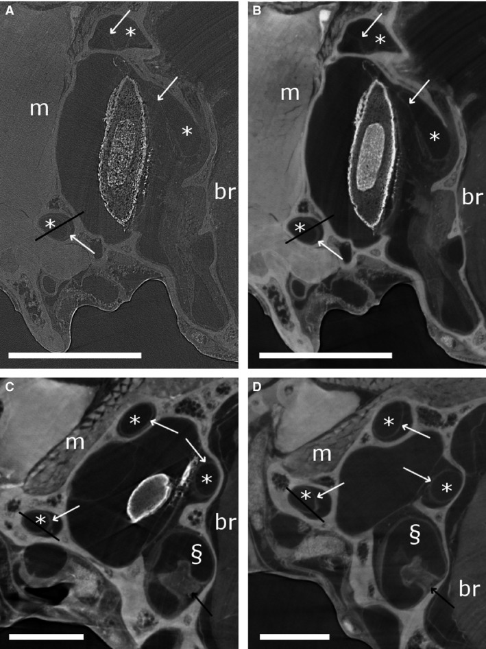
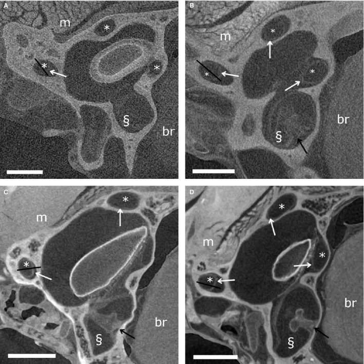
Synchrotron X‐ray micro‐tomography (μCT) transverse slices of Takydromus sexlineatus. (A and B) show the same slice, without (A) and after (B) phase retrieval. (C and D) show reconstructed slices after phase retrieval of the SYRMEP 3 and SYRMEP 4 scans, on which the cupula in the ampulla is visible. Scale bars: 0.5 mm. Semicircular canals (*), ampullas (§), brain tissue (br) and muscle tissue (m) are indicated. White arrows point to the membranous labyrinth, black arrows to cupulas. Black lines indicate the transects depicted in Fig. 2.

Figure 1B shows the same slice as in Fig. 1A after applying phase retrieval with the Paganin's method to the projection images. This substantially improves the contrast between the membranous labyrinth and the surrounding liquid (Fig. 1A,B). This is also apparent as a distinct peak on the grey‐scale value transects through the semicircular duct that was absent without phase retrieval (Fig. 2), and as an additional peak in the grey‐scale value histogram of the entire slice (Fig. 3). As a result, the CNR increases strongly (on average by a factor 4.95 ± 0.57; Fig. 4; Table 1). At the cost of a slight blurring effect, the grey‐scale difference between the membranes and the surrounding liquid becomes sufficiently large to enable a semi‐automatic segmentation in the 3D image manipulation software Amira. This allowed the creation of a 3D model of the membranous labyrinth (Fig. 5 and the image stack showed in Movie S1). The thickness of the membranes ranges between 2.71 and 26.84 microns in the synchrotron X‐ray μCT scans (average thickness of 12.01 ± 7.46 μm). The membranous walls are thickest at the inner side of the canal (towards the centre of the vestibular system), where most perilymph is present between the membranous labyrinth and the bony wall, and membrane thickness is minimal at the outer edge of the canal, where it attaches directly to the skull bone (Fig. 1B–D).

Figure 2.

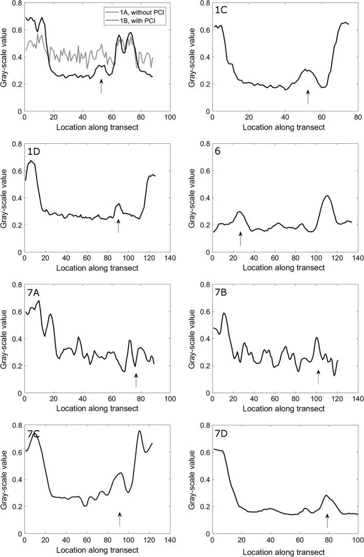
Grey‐scale values along the transect depicted by black lines on Figs 1, 6 and 7. Subplot numbering refers to the numbering in Figs 1, 6 and 7. The location of the membrane of the vestibular system is indicated by an arrow.

Figure 3.

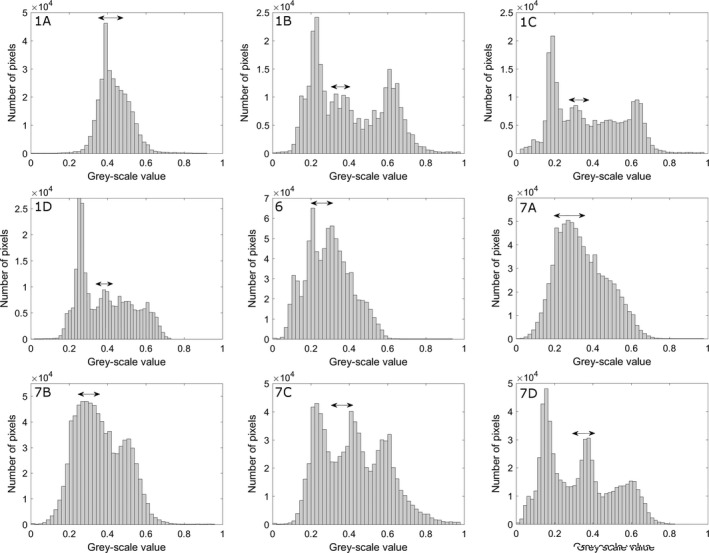
Histograms of the grey‐scale values present in the scans of Figs 1, 6 and 7. Subplot numbering refers to the numbering in Figs 1, 6 and 7. Double arrows indicate the range of grey‐scale values of the membranes of the vestibular system.

Figure 4.

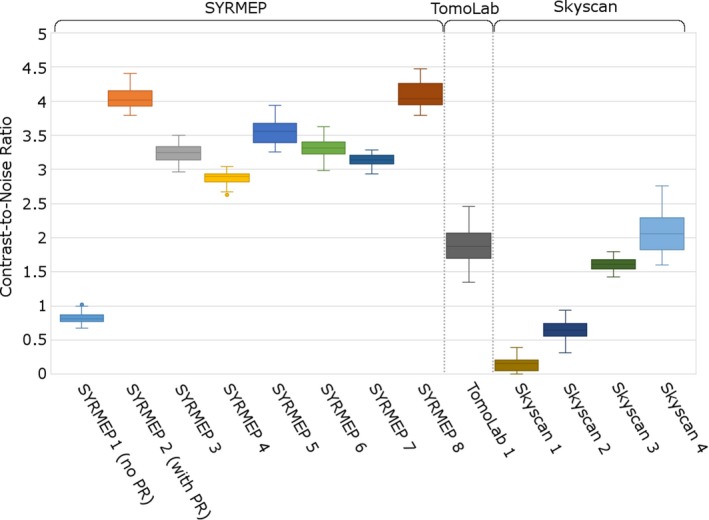
Boxplots showing the second and third quartiles, and the median of the contrast‐to‐noise ratio (CNR). The SYRMEP 1 and SYRMEP 2 datasets are based on the same scan, respectively, without and with phase retrieval (PR). Whiskers show the minimal and maximal values within the outlier range. Outliers are represented by dots.

Figure 5.

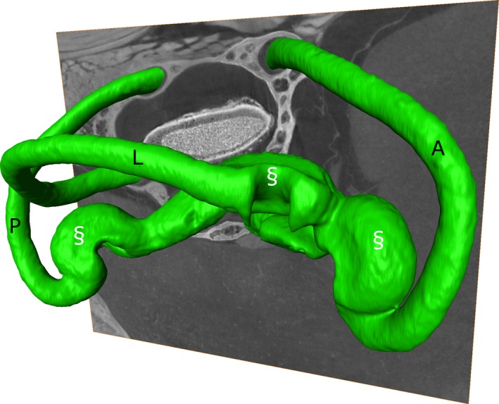
Isosurface rendering obtained after the segmentation of the membranous labyrinth (green) of Takydromus sexlineatus based on a synchrotron micro‐tomography (μCT) scan with phase retrieval (‘SYRMEP 2’; one sagittal slice is depicted). The lateral (L), anterior (A) and posterior (P) semicircular canals are indicated, as well as their ampullas (§).

Laboratory X‐ray μCT data

In Figs 6 and 7, we show representative slices of the different scans that we recorded with the microfocus X‐ray CT scanners (either the TomoLab station at Elettra or the commercially available Skyscan 1172 instrument).

Figure 6.

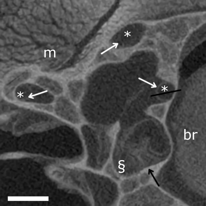
TomoLab laboratory X‐ray micro‐tomography (μCT) scan of Eremias bedriagae (transverse slice). Scale bars: 0.5 mm. Semicircular canals (*), the ampullas (§), brain tissue (br) and muscle tissue (m) are indicated. White arrows point to the membranous labyrinth, the black arrow points to the cupula. The black line indicates the transect depicted in Fig. 2.

Figure 7.

Skyscan laboratory X‐ray micro‐tomography (μCT) transverse slices. (A) Skyscan 1 scan of Phoenicolacerta laevis. (B) Skyscan 2 scan of Lacerta agilis. (C) Skyscan 3 scan of Takydromus sexlineatus. (D) Skyscan 4 scan of Takydromus sexlineatus. Scale bars: 0.5 mm. Semicircular canals (*), ampullas (§), brain tissue (br) and muscle tissue (m) are indicated. White arrows point to the membranous labyrinth, black arrows to cupulas. Black lines indicate the transects depicted in Fig. 2.

TomoLab set‐up

In the scans acquired with the TomoLab set‐up, the membranes of the relatively large E. bedriagae sample are well visible (Fig. 6). Also on the grey‐scale value transect, the membrane is clearly recognisable (Fig. 2). The vestibular system is relatively small (within the range of the T. sexlineatus specimens; Table 1) in this sample. The membranous walls are, however, considerably thicker (Table 1). The relatively high‐contrast resolution is partly due to the image acquisition protocol with a large sample‐to‐detector distance that exploits the advantages of PB‐PCI, even without applying phase retrieval. Because the CNR is lower than that of the synchrotron scans after phase retrieval (Fig. 4; Table 1), however, only manual (and not semi‐automatic) segmentation of the membranes and cupula is possible.

Skyscan instrument: comparison of scanning parameters

By carefully adjusting the scanning parameters of the Skyscan 1172 scanner, we could substantially improve the contrast of the membranous labyrinth. In the shortest scan (3 h 20 min, ‘Skyscan 1’), the membranous labyrinth is not (or hardly) visible inside the bony labyrinth (Figs 2 and 7A). The CNR is only 0.15 ± 0.10 (Table 1). This is not due to artefacts: no ring artefacts, motion artefacts or depletion artefacts were observed. When the scanning parameters are adjusted to resemble those of David et al. (2016), the membranous labyrinth becomes vaguely visible on a part, but not all, of the reconstructed slices (‘Skyscan 2’; Figs 2 and 7B). Also, the cupula in the ampulla is vaguely visible. The CNR remains low, though (Fig. 4; Table 1), and segmentation of the membranous labyrinth is not yet possible.

A much higher contrast of the membranes and the cupula in the ampulla is achieved for a smaller T. sexlineatus sample, for which the source voltage could be reduced from 100 kV to 60 kV (‘Skyscan 3’; Figs 2, 3 and 7C). Visual inspection shows that manual (but not semi‐automatic) segmentation becomes possible. The contrast is comparable to that of the TomoLab scan (CNR of 1.61 ± 0.09 for a larger specimen and, therefore, higher source voltage), and the membranes are even slightly sharper, also due to the smaller voxel size (Figs 4, 6 and 7C; Table 3). Reducing the source voltage even further to 40 kV amplifies this effect, leading to a CNR of 2.09 ± 0.31 (‘Skyscan 4’; Figs 4 and 7D). The elevated grey‐scale value of the membranes compared with the surrounding liquid is clearly recognisable at both the transects and the histograms of Skyscan 3 and Skyscan 4 (Figs 2 and 3).

Discussion

The purpose of our study was to compare several possible X‐ray μCT scanning protocols and tomographic reconstruction methods for the membranous labyrinth in small specimens (vestibular system < 4 mm). Despite the clinical and biological relevance of this organ, its study remains difficult because of the embedment in dense skull bone (Zachary & Mc Gavin, 2016), the thinness of the membranes (Curthoys et al. 1977; Wu & Wang, 2011), and the limited difference in X‐ray density between the membranes and the surrounding liquid (Rabbitt et al. 2004; Ekdale, 2016). As a result, most research on biological adaptations of the vestibular system is based on the anatomy of the bony labyrinth (Spoor et al. 2007; Cox & Jeffery, 2010; Malinzak et al. 2012; Georgi et al. 2013). However, investigation of the membranous labyrinth contributes valuable information because the fluid dynamics, which determine the functional properties of the system, are defined by the membranous labyrinth (Spoor et al. 2007; David et al. 2010).

Careful optimisation of the scanning parameters enabled good visualisation of the membranous labyrinth in even the smallest analysed samples (T. sexlineatus; smallest vestibular system size: 1.46 mm), both with conventional and with synchrotron‐based X‐ray μCT scanning. From a visual comparison of the images reported in the literature (Uzun et al. 2007; Wu & Wang, 2011; David et al. 2016; Johnson Chacko et al. 2018), the quality of the images obtained by our conventional μCT measurements is comparable to, or sometimes even better than, that of a larger specimen (including human, guinea pig, rhesus macaque and squirrel monkey specimens). The samples were decalcified in one of the investigations (Johnson Chacko et al. 2018), but our results as well as the other cited investigations show that this step can be omitted, avoiding artefacts. Further, our results, together with those of David et al. (2016), show that PTA staining performs as well as osmium tetroxide staining [used by Wu & Wang (2011), Uzun et al. (2007) and Johnson Chacko et al. (2018)]. Hence, the use of the volatile, toxic and expensive osmium tetroxide staining can be circumvented (Metscher, 2009).

The cited literature reports on conventional μCT set‐ups. Our study shows that the CNR of the membranous labyrinth can be enhanced further by using synchrotron radiation. We found that the best contrast of the membranous labyrinth can be achieved by acquiring a phase‐contrast synchrotron μCT scan followed by the application of a single‐distance phase‐retrieval algorithm to the sample projections (Paganin et al. 2002), prior to the tomographic reconstruction (Fig. 1; Table 1). The contrast is good enough to enable semi‐automatic segmentation of the thin membranes in 3D image manipulation software (such as Amira; Fig. 5). This makes a 3D modelling of the system and comparative analyses based on μCT data feasible. PCI achieved superior contrast because it relies on differences in the refractive index of materials, rather than on differences in the X‐ray attenuation thereof. Our results confirm that this is particularly beneficial for the visualisation and subsequent image segmentation of the soft tissue, which is known to have very little variation in X‐ray density. Moreover, using PCI, it is, in principle, possible to detect objects that are smaller than the image pixel size (Cloetens et al. 1997), which makes it even more promising for the visualisation of thin structures, such as membranes. We found a membrane thickness < 3 μm at some places, which is considerably less than the 10–50 μm thickness that was previously described in the literature (Curthoys et al. 1977; Rabbitt et al. 2004; Wu & Wang, 2011). Next to the higher spatial coherence of the X‐ray beam, allowing to benefit from strong phase‐contrast effects in X‐ray images, a further advantage of synchrotron X‐ray μCT set‐ups over conventional μCT scanners is the shorter scanning time due to the higher photon flux. This is not only convenient from the point of view of the operator, but it also decreases artefacts due to sample drying during scanning. Furthermore, shorter scans with limited radiation doses may even enable in vivo scanning at some point (Astolfo et al. 2013; Mohammadi et al. 2014).

Despite the clear advantages of synchrotron X‐ray μCT scanning, it is important that the membranous labyrinth can also be visualised using conventional μCT scanners in a laboratory setting (Wu & Wang, 2011; David et al. 2016). The protocols employed for the TomoLab and Skyscan scans (Table 3) benefit from phase‐contrast effects (albeit to a lesser extent than in synchrotron set‐up) due to the relatively large distance between source, sample and detector. No additional optical elements were necessary, as is the case for grating‐based PCI. We found that the average CNR of the TomoLab scan of the (relatively large) E. bedriagae sample is 65% of the lowest CNR of the synchrotron‐based scanner (Table 1).

Commercially available X‐ray μCT scanners with a conventional microfocus source generally have smaller distances between source, sample and camera due to their compact design. This reduces the phase‐contrast effects, but we selected the longest possible source‐to‐sample and sample‐to‐detector distances that were compatible with the selected magnification in our measurements (Table 3). Nevertheless, we found that a careful optimisation of the scanning parameters enables the visualisation of the membranous labyrinth even in very small T. sexlineatus samples (vestibular system size < 3 mm). It is worthwhile to invest in additional frame averaging and a small rotation step in order to reduce noise (BrukerMicroCT 2014). Scanning with an angular range of 360 ° also improves the contrast compared with 180 ° scanning, but reducing the source voltage proved to be much more beneficial to improve contrast. Especially in small specimens, for which sufficient transmission can be obtained at lower voltages, voltage reduction can improve contrast. This is probably due to an increase of the relative importance of the phase‐contrast effects. The lowest source voltage tested (40 V) resulted in a CNR that is very similar to that of the TomoLab scan (which concerns a larger specimen and, consequently, has a higher source voltage; Fig. 4; Tables 1 and 3). The reduced source voltage does, however, imply investing in a long exposure time (elongating the scan) even though the sample is smaller. Nevertheless, in many cases, it will be necessary or preferable to use a conventional μCT scanner, as this is less expensive and easier and faster to access compared with synchrotron facilities.

Conflict of interest

The authors declare no competing or financial interests.

Author contributions

JG, LM and JS designed this study; JG, MVK, RC and LM performed the scans; JG analysed the data; JG, LM and JS interpreted the data; all authors drafted the manuscript.

Supporting information

Movie S1. Transverse image stack of a synchrotron micro‐tomography (μCT) scan of Takydromus sexlineatus with phase retrieval (‘SYRMEP 2’). The green isosurface rendering shows the segmentation of the membranous labyrinth.

References

- Agrawal Y, Carey JP, Della Santina CC, et al. (2009) Disorders of balance and vestibular function in US adults. Arch Intern Med 169, 938–944. [DOI] [PubMed] [Google Scholar]
- Albers J, Markus MA, Alves F, et al. (2018) X‐ray based virtual histology allows guided sectioning of heavy ion stained murine lungs for histological analysis. Sci Rep 8, 1–10. [DOI] [PMC free article] [PubMed] [Google Scholar]
- Angelaki DE, Cullen KE (2008) Vestibular system: the many facets of a multimodal sense. Annu Rev Neurosci 31, 125–150. [DOI] [PubMed] [Google Scholar]
- Arnold EN (1998) Structural niche, limb morphology and locomotion in lacertid lizards (Squamata, Lacertidae); a preliminary survey. Bull Nat Hist Mus Zool Ser 64, 63–89. [Google Scholar]
- Astolfo A, Schültke E, Menk RH, et al. (2013) In vivo visualization of gold‐loaded cells in mice using x‐ray computed tomography. Nanomedicine 9, 284–292. [DOI] [PubMed] [Google Scholar]
- Brandt T, Dieterich M (2017) The dizzy patient: don't forget disorders of the central vestibular system. Nat Rev Neurol 13, 352–362. [DOI] [PubMed] [Google Scholar]
- Bravin A (2003) Exploiting the x‐ray refraction contrast with an analyser: the state of the art. Journal of Physics D: Applied Physics 36, A24–A29. [Google Scholar]
- BrukerMicroCT (2014) Bruker microCT method note: Workflow SkyScan 1172.
- Brun F, Mancini L, Kasae P, et al. (2010) Pore3D: a software library for quantitative analysis of porous media. Nucl Instrum Methods Phys Res, Sect A 615, 326–332. [Google Scholar]
- Brun F, Pacilè S, Accardo A, et al. (2015) Enhanced and flexible software tools for X‐ray computed tomography at the Italian synchrotron radiation facility Elettra (eds Dulio P, Frosini A, Rozenberg G). Fundam Inform 141, 233–243. [Google Scholar]
- Brun F, Massimi L, Fratini M, et al. (2017) SYRMEP Tomo Project: a graphical user interface for customizing CT reconstruction workflows. Adv Struct Chem Imaging 3, 4. [DOI] [PMC free article] [PubMed] [Google Scholar]
- Bushberg JT, Seibert JA, Leidholdt EM Jr, et al. (2002) The Essential Physics of Medical Imaging. Philadelphia: Lippincott Williams & Wilkins. [Google Scholar]
- Buytaert J, Goyens J, De Greef D, et al. (2014) Volume shrinkage of bone, brain and muscle tissue in sample preparation for micro‐CT and light sheet fluorescence microscopy (LSFM). Microsc Microanal 20, 1208–1217. [DOI] [PubMed] [Google Scholar]
- Cheriyedath S (2017) Micro‐MRI principles, strengths, and weaknesses. Available at: https://www.news-medical.net/life-sciences/Micro-MRI-Principles-Strengths-and-Weaknesses.aspx (accessed 6 November 2017).
- Cloetens P, Barrett R, Baruchel J, et al. (1996) Phase objects in synchrotron radiation hard x‐ray imaging. J Phys D: Appl Phys 29, 133–146. [Google Scholar]
- Cloetens P, Pateyron‐Salomé M, Buffière JY, et al. (1997) Observation of microstructure and damage in materials by phase sensitive radiography and tomography. J Appl Phys 81, 5878–5886. [Google Scholar]
- Costeur L, Mennecart B, Müller B, et al. (2017) Prenatal growth stages show the development of the ruminant bony labyrinth and petrosal bone. J Anat 230, 347–353. [DOI] [PMC free article] [PubMed] [Google Scholar]
- Cox PG, Jeffery N (2010) Semicircular canals and agility: the influence of size and shape measures. J Anat 216, 37–47. [DOI] [PMC free article] [PubMed] [Google Scholar]
- Curthoys IS, Blanks RH, Markham CH (1977) Semicircular canal radii of curvature (R) in cat, guinea pig and man. J Morphol 151, 1–15. [DOI] [PubMed] [Google Scholar]
- Dabov K, Foi A, Katkovnik V, et al. (2007) Image denoising by Sparse 3‐D transform‐domain collaborative filtering. IEEE Trans Image Process 16, 2080–2095. [DOI] [PubMed] [Google Scholar]
- David R, Droulez J, Allain R, et al. (2010) Motion from the past. A new method to infer vestibular capacities of extinct species. CR Palevol 9, 397–410. [Google Scholar]
- David R, Stoessel A, Berthoz A, et al. (2016) Assessing morphology and function of the semicircular duct system: introducing new in‐situ visualization and software toolbox. Sci Rep 6, 32 772. [DOI] [PMC free article] [PubMed] [Google Scholar]
- Descamps E, Sochacka A, De Kegel B, et al. (2014) Soft tissue discrimination with contrast agents using micro‐ct scanning. Belg J Zool 144, 20–40. [Google Scholar]
- Dullin C, Ufartes R, Larsson E, et al. (2017) μCT of ex‐vivo stained mouse hearts and embryos enables a precise match between 3D virtual histology, classical histology and immunochemistry. PLoS ONE 12, 1–15. [DOI] [PMC free article] [PubMed] [Google Scholar]
- Ekdale EG (2016) Form and function of the mammalian inner ear. J Anat 228, 324–337. [DOI] [PMC free article] [PubMed] [Google Scholar]
- Feldkamp LA, Davis LC, Kress JW (1984) Practical cone‐beam algorithm. J Opt Soc Am A 1, 612. [Google Scholar]
- Fitzgerald R (2000) Phase ‐sensitive X‐ray imaging. Phys Today 53, 23–26. [Google Scholar]
- Galiová M, Kaiser J, Novotný K, et al. (2010) Investigation of the osteitis deformans phases in snake vertebrae by double‐pulse laser‐induced breakdown spectroscopy. Anal Bioanal Chem 398, 1095–1107. [DOI] [PubMed] [Google Scholar]
- Georgi JA, Sipla JS, Forster CA (2013) Turning semicircular canal function on its head: dinosaurs and a novel vestibular analysis. PLoS ONE 8, e58517. [DOI] [PMC free article] [PubMed] [Google Scholar]
- Grohé C, Tseng ZJ, Lebrun R, et al. (2016) Bony labyrinth shape variation in extant Carnivora: a case study of Musteloidea. J Anat 228, 366–383. [DOI] [PMC free article] [PubMed] [Google Scholar]
- Herman GT (1980) Image Reconstruction from Projections. New York: Academic Press. [Google Scholar]
- Huang S, Kou B, Chi Y, et al. (2015) In‐line phase‐contrast and grating‐based phase‐contrast synchrotron imaging study of brain micrometastasis of breast cancer. Sci Rep 5, 9418. [DOI] [PMC free article] [PubMed] [Google Scholar]
- Ifediba MA, Rajguru SM, Hullar TE, et al. (2007) The role of 3‐canal biomechanics in angular motion transduction by the human vestibular labyrinth. Ann Biomed Eng 35, 1247–1263. [DOI] [PMC free article] [PubMed] [Google Scholar]
- Johnson Chacko L, Schmidbauer DT, Handschuh S, et al. (2018) Analysis of vestibular labyrinthine geometry and variation in the human temporal bone. Front Neurosci 12, 1–13. [DOI] [PMC free article] [PubMed] [Google Scholar]
- Lareida A, Beckmann F, Schrott‐Fischer A, et al. (2009) High‐resolution X‐ray tomography of the human inner ear: synchrotron radiation‐based study of nerve fibre bundles, membranes and ganglion cells. J Microsc 234, 95–102. [DOI] [PubMed] [Google Scholar]
- Maddin HC, Sherratt E (2014) Influence of fossoriality on inner ear morphology: insights from caecilian amphibians. J Anat 225, 83–93. [DOI] [PMC free article] [PubMed] [Google Scholar]
- Malinzak MD, Kay RF, Hullar TE (2012) Locomotor head movements and semicircular canal morphology in primates. Proc Natl Acad Sci USA 109, 17 914–17 919. [DOI] [PMC free article] [PubMed] [Google Scholar]
- Mancini L, Reiner E, Cloetens J, et al. (1998) Investigation of defects in AlPdMn icosahedral quasicrystals by combined synchrotron X‐ray topography and phase radiography. Philos Mag A 78, 1175–1194. [Google Scholar]
- Mancini L, Dreossi D, Fava C, et al. (2007) TOMOLAB: The nex X‐ray microtomographic facility @ ELETTRA. Elettra Highlights 2006–2007, 128–129.
- Mayo SC, Stevenson AW, Wilkins SW (2012) In‐line phase‐contrast X‐ray imaging and tomography for materials science. Materials (Basel) 5, 937–965. [DOI] [PMC free article] [PubMed] [Google Scholar]
- Mennecart B, Costeur L (2016) Shape variation and ontogeny of the ruminant bony labyrinth, an example in Tragulidae. J Anat 229, 422–435. [DOI] [PMC free article] [PubMed] [Google Scholar]
- Metscher BD (2009) MicroCT for developmental biology: a versatile tool for high‐contrast 3D imaging at histological resolutions. Dev Dyn 238, 632–640. [DOI] [PubMed] [Google Scholar]
- Mohammadi S, Larsson E, Alves F, et al. (2014) Quantitative evaluation of a single‐distance phase‐retrieval method applied on in‐line phase‐contrast images of a mouse lung. J Synchrotron Radiat 21, 784–789. [DOI] [PMC free article] [PubMed] [Google Scholar]
- Paganin D, Mayo SC, Gureyev TE, et al. (2002) Simultaneous phase and amplitude extraction from a single defocused image of a homogeneous object. J Microsc 206, 33–40. [DOI] [PubMed] [Google Scholar]
- Polacci M, Burton MR, La Spina A, et al. (2009) The role of syn‐eruptive vesiculation on explosive basaltic activity at Mt. Etna, Italy. J Volcanol Geoth Res 179, 265–269. [Google Scholar]
- Rabbitt RD, Damiano ER, Grant WJ (2004) Biomechanics of the semicircular canals and otolith organs In: The Vestibular System (eds Highstein SM, Fay RR.), pp. 153–201. New York: Springer. [Google Scholar]
- Rau C, Robinson IK, Richter C‐P (2006) Visualising soft tissue in the mammalian cochlea with coherent hard x‐rays. Microsc Res Tech 69, 660–665. [DOI] [PubMed] [Google Scholar]
- Rau C, Hwang M, Lee WK, et al. (2012) Quantitative X‐ray tomography of the mouse cochlea. PLoS ONE 7, e33568. [DOI] [PMC free article] [PubMed] [Google Scholar]
- Rau TS, Würfel W, Lenarz T, et al. (2013) Three‐dimensional histological specimen preparation for accurate imaging and spatial reconstruction of the middle and inner ear. Int J Comput Assist Radiol Surg 8, 481–509. [DOI] [PMC free article] [PubMed] [Google Scholar]
- Richter CP, Shintani‐Smith S, Fishman A, et al. (2009) Imaging of cochlear tissue with a grating interferometer and hard X‐rays. Microsc Res Tech 72, 902–907. [DOI] [PubMed] [Google Scholar]
- Rigon L, Erik V, Fulvia A, et al. (2010) Synchrotron‐radiation microtomography for the non‐destructive structural evaluation of bowed stringed instruments. e‐Preserv Sci 7, 71–77. [Google Scholar]
- Ruiz‐Yaniz M, Zanette I, Sarapata A, et al. (2016) Hard X‐ray phase‐contrast tomography of non‐homogeneous specimens: grating interferometry versus propagation‐based imaging. J Synchrotron Radiat 23, 1202–1209. [DOI] [PubMed] [Google Scholar]
- Saccomano M, Albers J, Tromba G, et al. (2018) Synchrotron inline phase contrast μCT enables detailed virtual histology of embedded soft‐tissue samples with and without staining. J Synchrotron Radiat 25, 1–9. [DOI] [PubMed] [Google Scholar]
- Schindelin J, Arganda‐Carreras I, Frise E, et al. (2012) Fiji: an open source platform for biological image analysis. Nat Methods 9, 676–682. [DOI] [PMC free article] [PubMed] [Google Scholar]
- Schultz JA, Zeller U, Luo Z‐X (2017) Inner ear labyrinth anatomy of monotremes and implications for mammalian inner ear evolution. J Morphol 278, 236–263. [DOI] [PubMed] [Google Scholar]
- Sijbers J, Postnov A (2004) Reduction of ring artifacts in high resolution micro‐CT reconstructions. Phys Med Biol 49, N247–N253. [DOI] [PubMed] [Google Scholar]
- Snigirev A, Snigireva I, Kohn V, et al. (1995) On the possibilities of x‐ray phase contrast by coherent high‐energy synchrotron radiations. Rev Sci Instrum 66, 5486–5492. [Google Scholar]
- Spoor F (2003) The semicircular canal system and locomotor behaviour, with special reference to hominin evolution. Courier Forschungsinstitut Senckenberg 243, 93–104. [Google Scholar]
- Spoor F, Garland T Jr, Krovitz G, et al. (2007) The primate semicircular canal system and locomotion. Proc Natl Acad Sci USA 104, 10 808–10 812. [DOI] [PMC free article] [PubMed] [Google Scholar]
- Tafforeau P, Boistel R, Boller E, et al. (2006) Applications of X‐ray synchrotron microtomography for non‐destructive 3D studies of paleontological specimens. Appl Phys A 83, 195–202. [Google Scholar]
- Tromba G, Longo R, Abrami A, et al. (2010) The SYRMEP Beamline of Elettra: clinical mammography and bio‐medical applications. In: AIP Conference Proceedings, pp. 18–23. Available at: http://aip.scitation.org/doi/abs/10.1063/1.3478190 (accessed 20 November 2017).
- Uzun H, Curthoys IS, Jones AS (2007) A new approach to visualizing the membranous structures of the inner ear – high resolution X‐ray micro‐tomography. Acta Otolaryngol 127, 568–573. [DOI] [PubMed] [Google Scholar]
- Vågberg W, Larsson DH, Li M, et al. (2015) X‐ray phase‐contrast tomography for high‐spatial‐resolution zebrafish muscle imaging. Sci Rep 5, 16 625. [DOI] [PMC free article] [PubMed] [Google Scholar]
- Wilkins SW, Gureyev TE, Gao D, et al. (1996) Phase‐contrast imaging using polychromatic hard X‐rays. Nature 384, 335–338. [Google Scholar]
- Wu C, Wang K (2011) Three‐dimensional models of the membranous vestibular labyrinth in the guinea pig inner ear. In: 4th International Conference on Biomedical Engineering and Informatics, pp. 544–547.
- Zachary JF, Mc Gavin MD (2016) Pathologic Basis of Veterinary Disease. Berlin, Germany: Elsevier Health Sciences. [Google Scholar]
Associated Data
This section collects any data citations, data availability statements, or supplementary materials included in this article.
Supplementary Materials