Rapid Compositional Mapping of Knee Cartilage with Compressed Sensing MRI

Abstract

More than one decade after the introduction of compressed sensing (CS) in MRI, researchers are still working on ways to translate it into different research and clinical applications. The greatest advantage of CS in MRI is the reduced amount of k-space data needed to reconstruct images, which can be exploited to reduce scan time or to improve spatial resolution and volumetric coverage. Efficient data acquisition using CS is extremely important for compositional mapping of the musculoskeletal system in general and knee cartilage mapping techniques in particular. High-resolution quantitative information about tissue biochemical composition could be obtained in just a few minutes using CS MRI. However, in order to make this goal a reality, some issues still need to be addressed. In this paper, we review the current state of the art of CS methods for rapid compositional mapping of knee cartilage. Specifically, data acquisition strategies, image reconstruction algorithms, and data fitting models are discussed. Different CS studies for T₂ and T_1ρ mapping of knee cartilage are reviewed, with illustrative results. Future directions, opportunities, and challenges of rapid compositional mapping techniques are also discussed.

Summary:

Compressed sensing MRI is a leap forward for rapid compositional mapping techniques, especially for knee cartilage. There are still several points to be refined for effective practical use, but there is no doubt that it will transform compositional mapping of knee cartilage into a rapid and reliable source of quantitative information for clinicians and researchers, without degrading the quality of relaxation maps, and providing a more comfortable experience for patients.

INTRODUCTION:

MRI systems are extremely versatile, being able to provide anatomical, functional and biochemical images of the human body (1). Quantitative mapping reveals parameter values of the MR signal relaxation process, providing important information to assess tissue biochemical composition (2, 3). Relaxation times, such as spin-lattice relaxation time (T₁), spin-spin relaxation time (T₂), spin-lattice relaxation time in the rotating frame (T_1ρ), or even a combination of them can provide more quantitative information about tissue structural and biochemical composition. For human knee cartilage, quantitative relaxation mapping is able to reveal biochemical changes in cartilage composition before morphological changes occur (4, 5).

For osteoarthritis (OA), a recent meta-analysis has validated the reliability (compiling 58 studies) and discriminative ability (compiling 26 studies) of cartilage compositional MRI mapping in knee (6, 7), where T₂ and T_1ρ relaxometry demonstrated discrimination validity in mild OA. This can help us to detect early stages of OA (8, 9).

In order to obtain precise relaxation parameters for voxels in a region of interest with high spatial resolution, long scanning time is usually required (10–12). This may include a large number of samples in k-space and several time points of a particular relaxation process of interest. However, long acquisition time is expensive and leads to patient discomfort. Captured data are more susceptible to be corrupted by patient motion and the overall experience is stressful.

Conventional reduction of scan time generally leads to some kind of degradation in image quality, such as reduced spatial resolution and/or aliasing artifacts (1). For quantitative imaging, a reduction in the number of time points decreases the precision of the estimated relaxation parameters (10), especially for more complex models such as biexponential relaxation (11). Initial approaches to acquire fewer k-space samples, such as partial k-space and key-hole (13), have halved acquisition time compared to fully sampled acquisitions, which is a modest reduction for quantitative relaxation mapping. Parallel imaging using multiple receive coils can be used to reduce the number of k-space samples required for reconstruction, due to different spatial sensitivities of the coil elements. Also, the SNR is usually higher than the one obtained from a volume (body) coil. With these methods, each receive coil is able to capture a different sensitivity-weighted signal from the object. Aliasing from regular undersampling can be solved with methods such as simultaneous acquisition of spatial harmonics (SMASH) (14), sensitivity encoding (SENSE) (15), generalized autocalibrating partially parallel acquisitions (GRAPPA) (16), and others (17). Some of the multi-coil reconstruction methods, such as SENSE, require the coil sensitivities to be known or estimated by an auxiliary method, such as (18), usually using a fully sampled central area of k-space, which is fast to acquire. Parallel imaging has been used for knee cartilage (19, 20) with up to 3 and 4 (21) fold acceleration factors (AF), taking nearly 5 min for data acquisition.

Compressed sensing (CS) aims to reduce the number of k-space samples by exploiting compressibility or sparsity in an appropriate transform domain. In order to exploit sparsity, the undersampling process is designed in such a way that the introduced aliasing artifacts look like random noise (22–24), which can be effectively removed with a nonlinear operation that enforces for example sparsity on a vector, low rankness on a matrix and combinations of sparse and low-rank models (24–26). The AF using CS for knee cartilage varies in the literature, however, it can reach between an 8 to 10 fold when combined with parallel imaging (27, 28), taking around 3 min for data acquisition.

While this is theoretically sound, there are many details, such as the optimal k-space sampling scheme, the regularization function, and the reconstruction algorithm, that need to be set correctly for efficient and widespread applications. In this paper, we will review the currently existing state-of-the-art compressed sensing approaches for rapid quantitative, compositional mapping of the knee cartilage.

The next section provides an overview of CS background including image data acquisition, image reconstruction from undersampled data, fitting models and parameters recovery. The following section briefly reviews the different CS studies for compositional T₂ and T_1ρ mapping of knee cartilage with illustrative examples. In the final section, future directions, opportunities, and challenges of rapid compositional mapping techniques are discussed.

REVIEW OF COMPRESSED SENSING MRI FOR COMPOSITIONAL MAPPING:

Theoretical Background:

Over the last decade, compressed sensing (24, 29), also known as compressive sampling (30, 31) was consolidated as an important breakthrough in sampling theory. It requires three specific ingredients: 1) sparse image representation (32), which states an image could be sparsely represented in a transformed domain, such as wavelet domain (33); 2) incoherent sampling (29, 30), which states any element in the sparse representation domain spreads almost uniformly (like a random noise) in the sampling domain, i.e. k-space; and 3) nonlinear image reconstruction (34), that exploits sparsity and incoherence to stably recover the exact image.

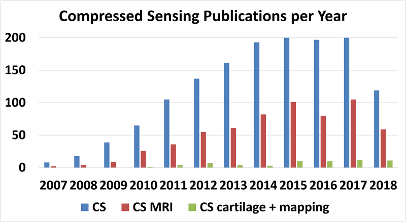
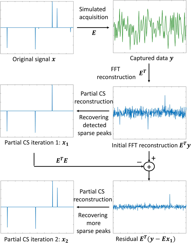
The field of MRI rapidly adopted compressed sensing (24) as shown in Figure 1, since k-space, is largely incoherent with the spatial domain (34) and with the domain defined by typical sparsifying transforms (22). In other words, when k-space is undersampled incoherently, the resulting aliasing artifacts look like noise in the sparse domain, rather than a structured artifact. This is exactly why sparse reconstruction works well, the sparse peaks are easily distinguishable and the noise-like artifact can be removed, as illustrated in Figure 2.

Figure 1:

Publications per year in the PubMed database related to compressed sensing (CS) in general, compressed sensing and magnetic resonance imaging (CS-MRI), and CS of cartilage and mapping (CS cartilage + mapping). Less than 8% of CS MRI publications are related to quantitative mapping or cartilage imaging.

Figure 2:

General concept used in CS. The original signal x should be sparse, and the system matrix E should be incoherent. The effect of this is that E^Ty, where y is the k-space data and E^T is the adjoint of E, should be basically sparse peaks mixed with noise-like artifacts, which are easily recovered by a nonlinear CS reconstruction. Most significant peaks are usually recovered at the initial iteration ${\widehat{\mathit{x}}}_1$. However, remaining sparse elements can be seen when the residual is mapped back to image domain, via ${\mathit{E}}^T(\mathit{y}-\mathit{E}{\widehat{\mathit{x}}}_1)$, and they are recovered in the following iterations, such as ${\widehat{\mathit{x}}}_2$.

From the practical point of view, it is not clear what the ideal sparse representation, i.e. sparsifying transform, for a sequence of relaxation-weighted images involving the knee cartilage area would be. In addition, the ideal sampling pattern should have minimum coherence between k-space and the sparse representation, which means these choices are connected. Next, we review the choices that have been found in the literature for knee cartilage mapping.

Data Acquisition:

In general, quantitative mapping of knee cartilage requires capturing multiple weighted images of a particular relaxation process of interest. The more the number of weighted images, the better the precision of the estimated parameter (35) with the penalty of long acquisition time.

Most current MRI sequences use contrast-preparation RF pulses followed by the imaging readout (36). The contrast-preparation pulses manipulate the spins in order to control the object with the appropriate magnetization that leads to the desired relaxation-weighted image. The imaging readout pulses generate phase and frequency encoding at the relaxation-weighted object in such a way its captured data lies in appropriate k-space position for further reconstruction (1). Usually, only a small portion of the k-space is captured after contrast-preparation, then the process is repeated until enough k-space samples are collected. Special attention is given to components located in the central area of the k-space (low-frequency components). They are usually captured first after magnetization preparation when the signal is strong and less deteriorated by imperfections of main magnetic field or gradient system (36).

T₂ mapping sequences can be based on both two-dimensional (2D) or on three-dimensional (3D) pulse sequences. In general, 2D sequences have limited volume coverage and often have poor through plane resolution compared to 3D sequences. However, 3D sequences usually come at the cost of a significant increase in scan time. MRI sequences such as 2D-multi-echo spin-echo (MESE) (37) has been utilized for CS studies in (38, 39) for T₂ weighting. Recently, however, 3D sequences such as double-echo steady-state (DESS) (40), triple-echo steady-state (TESS) (41), and a modified Turbo-FLASH or spoiled gradient echo (SPGR) sequences with T₂ preparation module have been used in (11, 42), respectively. The 3D sequences are preferred over 2D-MESE sequences due to stimulated echoes, magnetization transfer and diffusion effects (37, 43, 44). For T_1ρ weighting, relaxation preparation pulses (45) are applied before a sequence of gradient echo pulses for phase and frequency encoding. The sequence Magnetization-Prepared Angle-Modulated Partitioned k-Space Spoiled Gradient Echo Snapshots (MAPSS) (46) was used in some CS studies (47, 48), while in other CS studies (27, 49) a T_1ρ preparation module has been combined with a modified Turbo-FLASH sequence (12).

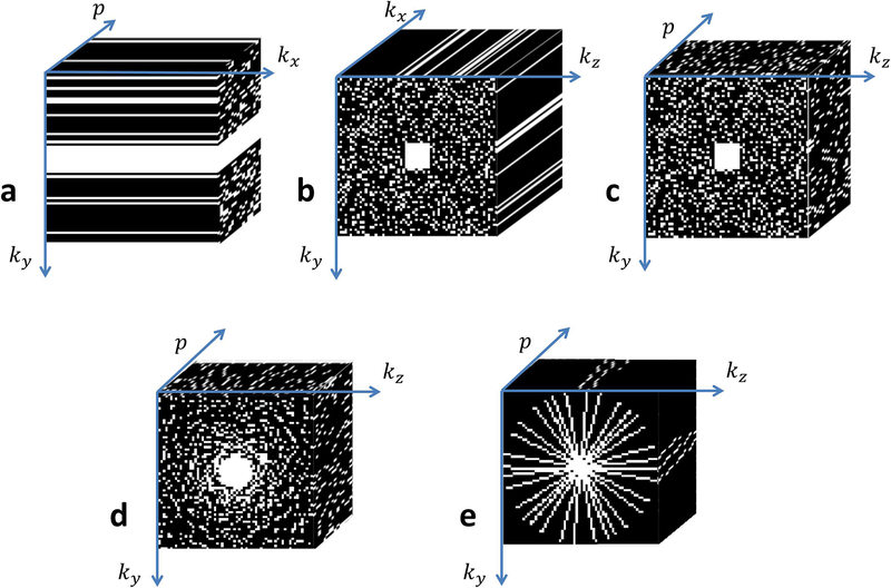
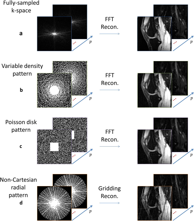
Compressed sensing exploits the concept of k-space undersampling, this is, encoding fewer points than required by the Nyquist sampling rate. In multislice 2D Cartesian acquisitions, 2D k-space from each slice is randomly undersampled along the phase-encoding (k_y) dimension only, since undersampling the frequency encoding direction (k_x) does not save scan time. In this case, phase encoding direction is undersampled in a random fashion, as shown in Figure 3(a). This sampling pattern is used in (39, 48, 50, 51). Since many relaxation-weighted images have to be captured to reconstruct relaxation maps, the acquisition process is repeated several times. CS works more efficiently in higher dimensional spaces, which are inherently more compressible, therefore the time of the relaxation process is treated as a third dimension (denoted by p) and random sampling pattern in the resulting k_y × p space (50) is considered jointly. The most commonly used undersampling pattern for this k_y × p space is the 2D Poisson disk, with some small fully sampled area in the central part of the k-space (52), as shown in Figure 3(a). When 3D k-space acquisitions are performed, one of the encoding directions is chosen as a readout (k_x), and it is fully sampled. The other two encoding directions, say k_y and k_z, which are phase encoded, are undersampled. In most of the cases, we preserve a central area of k-space, such as used in (27), and undersampling the remaining outer k-space area, either using 2D Poisson disk sampling (53), as shown in Figure 3(b), or Gaussian random sampling combined with regular undersampling (47), or even radially variable density (54), as shown in Figure 3(d). The 2D k_y × k_z undersampling pattern is usually different if looked at the p direction, as shown in Figure 3(c) for a 3D Poisson disk. The visual effect of noise-like aliasing artifacts of variable density and Poisson disk patterns are seen in Figures 4(b) and 4(c).

Figure 3:

Typical k-space sampling patterns utilized in compressed sensing for mapping of the knee cartilage. (a) 2D acquisitions for one slice, p is the relaxation parameter direction and k_x is the readout direction, where k_y × p is randomly undersampled with Poisson disk in the mid-high frequencies. (b) 3D acquisition for one relaxation-weighted volume and (c) for one slice in the x direction (after FFT in k_x direction) the k_y × k_z × p sampled points follow a 3D Poisson disk pattern. (d) The sample points follow a radially variable density pattern, and (e) radial sampling with golden angle increments and different initial angle for each p.

Figure 4:

Visual effect of the sampling pattern compared to (a) fully sampled knee images when FFT is used for reconstruction: (b) variable density pattern, with 45% of k-space sampled, (c) Poisson disk pattern, also with 45% of k-space sampled, and (d) radial pattern with 40% of k-space sampled.

Radial k-space acquisition is usually more robust to motion artifacts, and acquisition signal to noise ratio (SNR) are a little higher due to sampling of the central k-space position at every readout (55), as seen in Figure 3(e). Radial acquisitions do not fall onto the Cartesian grid and requires gridding for reconstruction (56). For iterative reconstructions, the non-uniform fast Fourier transform (NUFFT) (57) is usually employed (58, 59), which increases computation time. So far, radial sampling had only been applied to T₂ mapping (60) and sodium MRI (61) for knee cartilage. The visual effects of noise-like aliasing artifacts of radial sampling are seen in Figure 4(d).

The number of temporal points in the p direction (echo time (TE) for T₂ mapping or length of spin-lock time (TSL) for T_1ρ mapping) and their distribution chosen to measure the relaxation process are extremely relevant, especially if the expected behavior of the relaxation process is not monoexponential (62). Optimal time spacing has been discussed in (35) for T₂, while efficient sampling in (10) for T_1ρ. However, it has never been discussed how CS affects the choice of temporal sampling points.

Image Reconstruction from Undersampled Data:

Compressed sensing reconstruction is an inverse problem that aims to recover an image that is sparse in some transformed domain using undersampled data only. The reconstruction problem can be formulated as:

$$\widehat{\mathit{x}}={\text{argmin}}_{\mathit{x}}{‖\mathit{y}-\mathit{E}\mathit{x}‖}_{\mathbf{2}}^{\mathbf{2}}+\lambda \mathit{R}\left(\mathit{x}\right),$$ [1]

where x is a vector that represents the reconstructed set of relaxation-weighted images, with its original size of N_y × N_z × p, y is a vector that represents the captured k-space data for all relaxation-weighted images, its original size is k_y × k_z × c × p, where c is the number of receive coils, and the matrix E represents the encoding matrix mapping x to y, containing coil sensitivities (when parallel imaging and CS is jointly used (64)), Fourier transforms, and sampling pattern (27). Many CS methods for knee cartilage use the joint parallel imaging and CS approach to achieve higher undersampling rates, as shown in (27, 28, 47, 48, 65). The use of squared l₂-norm, or Euclidean norm, ${‖\mathit{e}‖}_2^2={\sum }_{i=1}^N{\left|e_i\right|}^2$, is quite common either because it is related to the usual assumption of Gaussian noise (63), or because it leads to a more tractable mathematical problem. Also, in [1], λ is the regularization parameter and R(x) is the regularization function.

Sparsity is a key assumption for CS image recovery. In [1], sparsity is induced by the regularization function R(x). Typically, $\mathit{R}\left(\mathit{x}\right)=\Vert {\mathit{T}}_{\mathit{x}}{\Vert }_1$ is utilized, where the l₁-norm, ${‖\mathit{u}‖}_1={\sum }_{i=1}^M\left|u_i\right|$, is small for sparse, or nearly sparse u vectors, and u = Tx, where T is a sparsifying transform. The size of u depends on the chosen T. Wavelet transforms or finite differences are commonly used as spatial sparsifying transforms. However, as the set of relaxation-weighted images are jointly reconstructed, as x, more sophisticated temporal or spatiotemporal models can be used. In order to deal with the higher correlation between relaxation-weighted images, temporal model-based learned dictionaries from Principal Component Analysis (PCA) or K-means Singular Value Decomposition (K-SVD), or even 3D wavelet (2D+time) and spatiotemporal finite differences (60, 65, 66) are used. Figure 5 illustrates an example when only the top 15% coefficients are used to recover the images with 3D wavelet.

Figure 5:

Example of the sparsity or compressibility of the knee images in the 3D wavelet (2D+time) transformed domain. The original images x are sparse when transformed via Tx, such as wavelet transform. If only the top 15% of the coefficients are preserved, and the rest nulled, we can still recover a very similar image $\tilde{\mathit{x}}$ using inverse transform T⁻¹. The difference $\tilde{\mathit{x}}-\mathit{x}$ is usually very small and has a noise-like aspect.

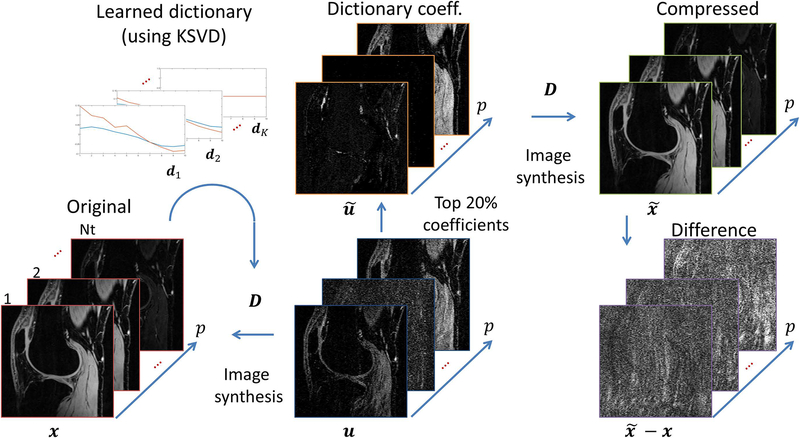
When a dictionary is learned simultaneously with the reconstructed image, the regularization $\mathit{R}\left(\mathit{x}\right)={‖\mathit{D}\mathit{u}-\mathit{P}\mathit{x}‖}_2^2,\mathrm{ }\mathrm{ }\mathrm{ }\mathrm{s}.\mathrm{t}.{‖\mathit{u}‖}_0\le T$ is usually used, as in (66). In this case, D is the dictionary, P is a patch selector, and ‖u‖₀ is the l₀-pseudonorm which defines the number of non-zero elements of u. One of the issues with this kind of regularization is that it is non-convex (due to l₀-pseudonorm) and may not produce stable solutions (34). If reference data or signal model is available, the dictionary can be learned before the reconstruction, using tools as K-SVD (50). Figure 6 illustrates as an example when K-SVD is used to learn an overcomplete temporal dictionary. Since the voxel representation over time is redundant (67), only some small number of coefficients can be used to reconstruct the image with very little difference.

Figure 6:

Example of the sparsity or compressibility of the knee images using a learned overcomplete temporal dictionary D. The dictionary atoms d_k can be learned from a model or the data itself using K-SVD, for example. The dictionary is usually redundant and x = Du is non-unique, but a sparse version $\tilde{\mathit{u}}$ can be found such that the difference $\tilde{\mathit{x}}-\mathit{x}$ is small.

Another kind of sparsity is produced by low rank models (38). One example is R(x) = ‖x‖_*, or the nuclear-norm (68) of x. Low rank models reshape the reconstructed image sequence in to a Casorati matrix, say X, with spatial position of the voxels oriented in one dimension and time position in the other. This matrix is usually of low rank.

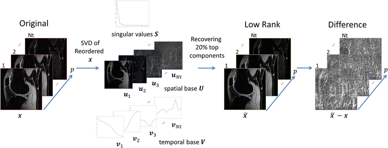
The singular values decomposition (SVD), such as X = VSU^T, where matrices V and U represents principal components in its columns, ordered by importance from left to right, where V contains spatial information and U relaxation (or time) signal information. The diagonal matrix S contains the singular values, which weights the components by its importance. If X is low rank, then only the first elements of the diagonal of S are significant (non-zero). Columns of V and U related to small elements of S can be removed without significant changes in X. In some sense, low rank model represents sparsity of the SVD structure of the matrix X, so the requirement of sparsity still holds true. Figure 7 illustrates low rank representation for knee cartilage images.

Figure 7:

Example of the low rank model for relaxation-weighted images. The “sparsity” of this model is in the singular values of the Casorati matrix of the images, as X = VSU^T. A reduced structure given by the principal components of the SVD, using only the first and most significant components of U = [u₁,.., u_Nt], V = [v₁,..,v_Nt], and S = diag(s1,…,s_Nt), reconstructs $\tilde{\mathit{X}}$ which yields a signal $\tilde{\mathit{x}}\mathit{ }$ with very small difference $\tilde{\mathit{x}}-\mathit{x}$.

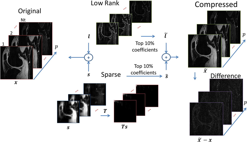
Many recent studies (26, 27) observed that low rank models can be combined with some typical sparse representation in such a way that both could be used to represent the reconstructed signal. This gave rise to low rank plus sparse (L+S) models where $\lambda \mathit{R}\left(\mathit{x}\right)={{\lambda }_{\mathit{l}}‖\mathit{l}‖}_{\mathit{*}}+{\lambda }_{\mathit{s}}{‖\mathit{T}\mathit{s}‖}_1$, being x = l + s, were s is the sparse part, using the l₁-norm to induce sparsity, and when l is the low rank part, based on the nuclear-norm. This is also an overcomplete representation of the image, as illustrated in Figure 8. Having so many options for regularization functions may be confusing. In (27), twelve different variations were compared for T_1ρ mapping, concluding that 3D finite difference for T, or exponential dictionary for D, or 2D finite difference for T in the L+S model were among the best for the problem.

Figure 8:

Illustration of the low rank (L) plus sparse (S) decomposition, which combines two models: the low rank and sparse, as x = s + l. Note the sparse component s can, actually, be sparse in a domain given by a sparsifying transform T, 2D wavelet in this case. If only the top 10% of the sparse coefficients are preserved to generate $\tilde{\mathit{s}}$ and the top 10% principal components are preserved to generate $\tilde{\mathit{l}}$, then a compressed $\tilde{\mathit{x}}=\tilde{\mathit{s}}+\tilde{\mathit{l}}$ can still represent x with very small difference $\tilde{\mathit{x}}-\mathit{x}$.

The cost function showed in [1] still needs to be solved by a minimization algorithm. The first compressed sensing approaches in MRI (22, 24, 69) and some that followed them (64) used nonlinear conjugate gradient (NLCG) (70). This is the most commonly used algorithm for CS in cartilage applications (47, 60, 61). NLCG is not very effective for problems with l₁-norm and definitely cannot handle low rank and low rank plus sparse models, requiring more sophisticated mathematical tools such as the proximal operator (71). Perhaps due to this, several customized CS algorithms had been used for knee cartilage, such as (28, 66). A negative point of customized algorithms is that convergence is not always mathematically analyzed, meaning it is not guaranty to work on different scanning configurations or initial values, for example. The use of well-studied algorithms such as alternating direction method of multipliers (ADMM) (72) or fast iterative shrinkage-thresholding algorithm (FISTA) (73, 74), used in (39) and (27) respectively, are somewhat safer from this point of view.

One important point left unanswered in most CS studies is the choice of the regularization parameters λ, or λ_s and λ_l. For feasibility tests, choosing the regularization parameter in order to have results similar to the fully sampled reconstructions makes sense, either by comparing image reconstruction error (27, 65) or estimated relaxation parameter error (75). In these cases, the fully sampled data is available for comparison. Nevertheless, in practical applications, when prospective undersampling needs to be done, this is still an open problem. Classical criteria that does not make use of any reference, such as L-curve (76), generalized cross-validation, or Stein’s unbiased risk estimate (77) remain untested for quantitative mapping of knee cartilage using CS.

Fitting Models and Parameters Recovery:

In general, relaxation processes are assumed to be exponentially decaying. Models based on magnitude decay are expressed as:

$$\left|x(t,\mathit{n})\right|=a\left(\mathit{n}\right)\text{exp}\left(-\frac{t}{\tau \left(\mathit{n}\right)}\right)+b$$ [2]

where x(t,n) is one particular voxel over time t at position n, a(n) is a positive real-valued measurement of the magnitude of the magnetization, and τ(n) is the relaxation decaying time at position n. The constant component b is included due to residual noise.

Multicomponent exponential models had also received more attention recently (78–80). Different exponential decaying time constants are observed in biological systems due to the presence of protons in different molecules. Biexponential model is usually the next step after monoexponential decaying (11, 12, 49, 81). But three components had already been reported in the literature (79, 82). It was also reported nonexponential decay in (83, 84) for knee cartilage, but there is not much investigation on it. Generally, multiexponential models can be written as:

$$\left|x(t,\mathit{n})\right|=a\left(\mathit{n}\right)\left[{\sum }_{j=1}^J{f}_j\left(\mathit{n}\right)\text{exp}\left(-\frac{t}{{\tau }_j\left(\mathit{n}\right)}\right)\right]+b,$$ [3]

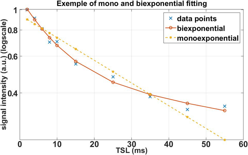
where τ_j(n) is the relaxation decaying time and f_j(n) is the fraction of the component j of the multicomponent exponential. Figure 9 illustrates the decaying measured in one voxel of a 3D-T_1ρ mapping of the human knee cartilage. Clearly, the biexponential model better represents the observations.

Figure 9:

Measured T_1ρ decaying signal from the knee cartilage. Different TSL Points were fitted with monoexponential and biexponential models. Biexponential provided a better fit with lower residual error than monoexponential model.

Multiexponential evaluation can also be obtained by a dictionary with fixed exponentials with different relaxation times τ_j, also known as an inverse Laplace transform (85), which can be written as:

$$\left|x(t,\mathit{n})\right|={\sum }_{j=1}^J{c}_j\left(\mathit{n}\right)\text{exp}\left(-\frac{t}{{\tau }_j}\right)+b,$$ [4]

In this case, only the coefficients c_j(n), related to exponential functions with times τ_j, need to be estimated.

Model fitting can be efficiently done with nonlinear least squares (NLS) (86). This is usually executed by voxel-by-voxel, and one can use it with any model, from monoexponential to multiexponential. However, NLS defines only the cost function (and the term nonlinear is due to the use of exponential models), an optimization algorithm is still necessary. The Levenberg-Marquardt (86) algorithm is the most commonly used for the fitting part of the quantitative mapping. It has been used in (48) for T_1ρ mapping and in (50) for T₁ and T₂ mapping with monoexponential models. The conjugate gradient Steihaug’s trust-region algorithm (87) is used in (27) for monoexponential and in (49) for biexponential T_1ρ mapping. In (39) the variable projection algorithm for NLS (88) is utilized for monoexponential T₁ and T₂ problems.

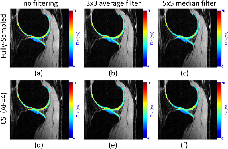
Spatial filtering before the fitting process is sometimes useful. This is typically done in non-CS approaches to reduce noise, but it is actually useful in CS approaches as well (27). Figure 10 illustrates some representative examples. When filtering is utilized, the error between the relaxation map obtained by a fully sampled reconstruction and CS reconstruction is much smaller. The price, however, is the lack of details in the obtained relaxation maps.

Figure 10:

Effect of pre-filtering the reconstructed knee joint images before the fitting process on T_1ρ mapping. In this example, CS method using Poisson disk pattern for sampling and spatiotemporal finite differences for regularization is utilized, according to (27).

APPLICATIONS OF CS-MRI TO COMPOSITIONAL MAPPING OF KNEE CARTILAGE:

T₂ Mapping:

T₂ mapping is perhaps the most studied for knee cartilage due to the availability of imaging sequences on all major vendors. It is known that T₂ is sensitive to water, collagen content and tissue anisotropy (43). In (6) is shown that T₂ is usually higher in knee OA patients, compared to healthy subjects, with significant differences between subjects (standardized mean difference of 0.49). The acceleration of T₂ mapping using compressed sensing was among the first applications for knee cartilage, where radial acquisition and PCA sparsity were used to demonstrate the possibility of reducing acquisition time by 8 times, requiring 2 min and 17 sec, with little loss compared to the gold standard (60).

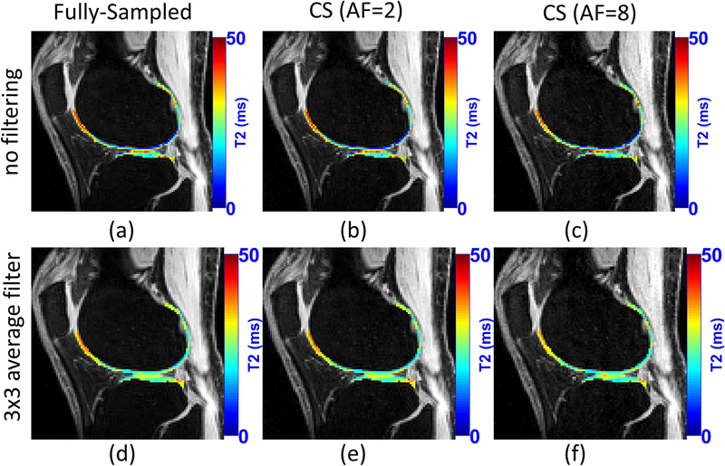
In (28), Peng et al. shown similar acceleration results for knee cartilage, but with multi-coil Cartesian sampling and a mix of sparsity and low rank priors. Nevertheless, specific error bounds for T₂ mapping of knee cartilage for different levels of acceleration are not precisely known yet. Figure 11 illustrates a comparison of T₂ mapping using CS. A list of studies on T₂ mapping of knee cartilage using CS is included in Table 1.

Figure 11:

A visual example of the acceleration provided by CS for T₂ mapping of knee cartilage. CS method used Poisson disk pattern for sampling and sparsity on exponential dictionaries. The use of filtering before fitting is also illustrated. Note that T₂ maps of knee cartilage after filtering is much smoother.

Table 1:

Publications related to compressed sensing MRI for rapid compositional mapping of the knee cartilage

Authors	Year	Application	Sampling Pattern	time points	Regularization	Reconstruction	Fitting
Madelin et. al	2012	Sodium	Radial	1	sparsifying transform + TV	nonlinear Conjugate Gradient	not reported
Huang et. al	2012	T2	Radial fast spin echo sequence	8 (echo spacing ~ 8.38 ms)	Sparse PCA, model based	nonlinear Conjugate Gradient	not reported
Peng et. al	2016	T2	Cartesian 2D multislice, k-p sampled as Poisson disk	10 (from TE=17 ms, echo spacing ~ 8.5 ms)	wavelet, casorati low rank, hankel low rank (nuclear norm)	Custom, alternated filtering and data-consistency	NLS
Pandit et. al	2016	T1ρ	Cartesian 3D, 2D center preserved, ARC + 2D Gaussian random	8 (TSL=0/2/4/8/12/20/40/80 ms)	modified total variation	nonlinear Conjugate Gradient	not reported
Zhou et. al	2016	T1ρ	Cartesian 2D multislice, k-p sampled as Poisson disk	8 (TSLs=0/2/4/8/12/20/40/80 ms)	Sparse PCA with (locally-adaptive iterative support detection)	FOCUSS algorithm	NLS -Levenberg-Marquardt fitting algorithm
Zibetti et. al	2018	T1ρ	Cartesian 3D, 2D center preserved, Poisson Disk (2D+ time)	10 (TSLs=2/4/6/8/10/15/25/35/45/55ms)	12 different methods (sparsity: wavelet, finite differences, PCA, KSVD; low rank, L+S with spatial, wavelet and finite difference sparsity)	FISTA, FISTA-FGP, and modified FISTA/FISTA-FGP	NLS - conjugate gradient Steihaug’s trust-region (CGSTR) algorithm
Wang et. al	2018	T1 - GAG - dGEMRIC	Cartesian 2D spin-echo imaging	5 (T= 0/0.4/1.1/2.2/4.0s) or (T=0/0.1/0.3/0.5/1.0s)	sparifying transform + TV	nonlinear Conjugate Gradient	Donnan equilibrium theory

T_1ρ Mapping:

T_1ρ is sensitive to proteoglycan content (89). The previous studies (6, 8, 90) have shown the potential of using T_1ρ to detect early biochemical changes in osteoarthritis. T_1ρ is also increased in patients with knee OA, demonstrating the best discriminatory ability for subjects with disease (6) (with standardized mean difference of 0.73). Due to its importance, acceleration of T_1ρ mapping using CS has been better studied than with T₂ in knee cartilage. See Table 1 for a list of studies on CS for knee cartilage mapping.

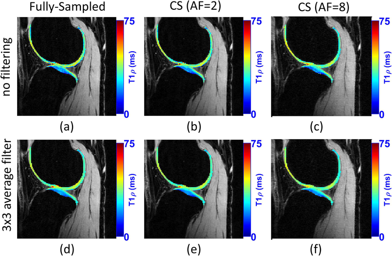
Pandit et al. combined CS with autocalibrating reconstruction for Cartesian sampling (ARC) in (47). They reported acceleration factors of 3 compared to the fully sampled acquisition, but the resulting acquisition time of 3 min is what is typically observed in other CS studies. In (48), a combined reconstruction with locally adaptive iterative support detection (k-t LAISD) and joint image reconstruction and sensitivity estimation in SENSE (JSENSE) method was proposed for knee cartilage, with AF up to 3 and 3.5. In (27, 49), Zibetti et al. showed a detailed comparison of twelve different regularization functions, where some of them are able to achieve error below 6.5% compared with maps produced by fully sampled k-space, but with AF of 10, resulting in 3.2 minutes of acquisition. Figure 12 illustrates a comparison of T_1ρ mapping using CS.

Figure 12:

A visual example of the acceleration provided by CS for T_1ρ mapping of knee cartilage. CS method used Poisson disk pattern for sampling and L+S with sparsity in the spatial finite difference, as shown in (27). The use of filtering before fitting is also illustrated. Similarly, T_1ρ maps of knee cartilage after filtering is much smoother.

Other Types of Mapping:

Madelin et al. applied compressed sensing to map sodium concentration in (61) for knee cartilage using radial acquisitions and combined wavelet and total variation sparsity constraints, to obtain an AF of 4 and reduce the acquisition from 20 min to 5 min. The signal-to-noise ratio is still an issue with sodium MRI. In (91), Behl et al. showed that repeating the same radial spokes, in a radial acquisition with a reduced number of angles followed by CS reconstruction, is better than capturing more angular points and reconstruct with gridding methods.

The delayed gadolinium-enhanced MRI of cartilage (dGEMRIC) (92) is sensitive to glycosaminoglycans (GAG), presenting different T₁ relaxation time in knee cartilage, which can also be used to detect cartilage degradation. In (54), Wang et al. applied compressed sensing to accelerate GAG quantization with ex-vivo microscopic MRI, achieving AF up to 16, reducing the scan time to ~8–30 min from fully sampled scans of ~2–8h.

FUTURE DIRECTIONS OF RAPID COMPOSITIONAL MAPPING OF KNEE CARTILAGE:

Open Questions for CS of Knee Cartilage:

Even though compressed sensing MRI is currently mature and vendors are starting to introduce commercial products, clinical and basic researchers still need to address many questions in order to fully exploit its benefits.

There is no consensus on a method to choose the number of relaxation time points of the relaxation process. Most studies regarding relaxation time points use only fully sampled acquisitions (10, 35). The problem is different when CS reconstruction is used. Just to elucidate some differences: the noise in the reconstructed images is no longer Gaussian, as shown in (27), and depends on the kind of regularization function utilized, among other factors. Ideal sampling time points also depend on expected tissue time decay and may change depending on the clinical study. In other words, we may expect to see more studies in this direction in the near future.

Another unanswered question is regarding the ideal k-space undersampling pattern. Poisson disk seems to be the dominant approach for multi-slice 2D and 3D acquisitions, but other optimized approaches with variable density, such as (93), may be better. New comparative studies on this point should be done in the future.

Regularization functions with learned sparsifying transforms or dictionaries have been reported in the literature (94). Learning dictionaries are already a reality (66) with knee cartilage mapping. However, instability due to non-convexity still needs to be resolved. Methods like blind compressed sensing (95, 96) are important steps in terms of learning sparsifying basis within a more stable optimization. Blind CS has been applied for brain mapping in (94).

Other Emerging Rapid Imaging Methods:

Model-based reconstruction is an interesting approach that has already produced good results for brain mapping using monoexponential models with 4 to 6 fold AF (97, 98). Essentially, the system matrix E from [1] is combined with the exponential model, similar to [2]–[4], usually leading to a nonlinear operator. Instead of reconstructing the image and then proceed to model fitting, the model-based reconstruction finds the parameters directly. Note that if a multiexponential linear model, similar to the inverse Laplace transform in [4] is utilized, it can be straightforwardly combined with CS, as illustrated in (27) for knee cartilage for 10 fold AF.

Another promising approach for multiple quantitative parameters is magnetic resonance fingerprinting (MRF) (99, 100). MRF uses a different approach, instead of varying one parameter and keeping the others fixed as in most quantitative imaging, it changes all acquisition parameters in a pseudorandom fashion such that each tissue generates a unique evolution, or “fingerprinting”, detected by a pattern recognition algorithm. This technique has been applied to rapid brain (99–101) and abdominal (102) mapping, but it can soon be applied to cartilage mapping as well.

Artificial intelligence methods that make use of deep learning (103), such as convolutional neural networks (104) and domain-transform manifold learning (105) are finding their way to imaging. These methods have been successfully applied to computed tomography (106) and MRI (107, 108), and recently used for compositional brain mapping (109). One challenge when using these methods is how to obtain the training data sets. Large fully sampled datasets may be required, but this is exactly what rapid acquisitions want to avoid. In (109) simulated signals were used to generate the training database with good results.

Challenges in prospective CS:

The quality of CS reconstruction depends on the right choice of the regularization parameters. In retrospective CS studies, the parameter is usually adjusted to provide an image as similar as possible to the fully sampled reference image. However, this is not possible in prospective studies. In this sense, methods for automatically choose the regularization parameters need to be studied.

Potential Advantages of CS MRI:

The most important advantage is the reduction of scan time. Considering the different studies presented here, on average, it is observed a reduction of acquisition time from ~20–30 min, required by a fully sampled scan, to ~3–5min, taken by a CS undersampled scan. These scan times are similar to the time required by most anatomical routine clinical acquisitions.

The benefits of the reduced scan time are many, from the economical point-of-view more patients can be examined per period of time; from the comfort point-of-view, patients do not need to stay still inside the scanner for long periods of time. The chances of the scanned data are corrupted by patient motion are smaller, but if data are corrupted, then an eventual repetition of the scan can be done without seriously affect scanner schedule. High-resolution mapping is possible without increasing acquisition time to much. More time points can be acquired, making studies with multiexponential models and evaluation of multi-relaxation mapping a reality in clinical practice and revealing more information about the biology and pathobiology of cartilage tissue, as well the effects of cartilage preserving therapies.

REFERENCES

- 1.Liang ZP, Lauterbur PC: Principles of Magnetic Resonance Imaging: A Signal Processing Perspective. IEEE Press; 2000. [Google Scholar]
- 2.Matzat SJ, van Tiel J, Gold GE, Oei EHG: Quantitative MRI techniques of cartilage composition. Quant Imaging Med Surg 2013; 3:162–174. [DOI] [PMC free article] [PubMed] [Google Scholar]
- 3.Ross R, Goodpaster B, Kelley D, Boada F: Magnetic resonance imaging in human body composition research. From quantitative to qualitative tissue measurement. Ann N Y Acad Sci 2000; 904:12–7. [DOI] [PubMed] [Google Scholar]
- 4.Binks DA, Hodgson RJ, Ries ME, et al. : Quantitative parametric MRI of articular cartilage: A review of progress and open challenges. Br J Radiol 2013:20120163. [DOI] [PMC free article] [PubMed] [Google Scholar]
- 5.Li X, Majumdar S: Quantitative MRI of articular cartilage and its clinical applications. J Magn Reson Imaging 2013; 38:991–1008. [DOI] [PMC free article] [PubMed] [Google Scholar]
- 6.MacKay JW, Low SBL, Smith TO, Toms AP, McCaskie AW, Gilbert FJ: Systematic review and meta-analysis of the reliability and discriminative validity of cartilage compositional MRI in knee osteoarthritis. Osteoarthr Cartil 2018. [DOI] [PubMed] [Google Scholar]
- 7.Link TM, Li X: Establishing compositional MRI of cartilage as a biomarker for clinical practice. Osteoarthr Cartil 2018:2–4. [DOI] [PubMed] [Google Scholar]
- 8.Regatte RR, Akella SVS, Lonner JH, Kneeland JB, Reddy R: T1ρ relaxation mapping in human osteoarthritis (OA) cartilage: Comparison of T1ρ with T2. J Magn Reson Imaging 2006; 23:547–553. [DOI] [PubMed] [Google Scholar]
- 9.Li X, Benjamin Ma C, Link TM, et al. : In vivo T1ρ and T2 mapping of articular cartilage in osteoarthritis of the knee using 3T MRI. Osteoarthr Cartil 2007; 15:789–797. [DOI] [PMC free article] [PubMed] [Google Scholar]
- 10.Johnson CP, Thedens DR, Magnotta VA: Precision-guided sampling schedules for efficient T1ρ mapping. J Magn Reson Imaging 2015; 41:242–250. [DOI] [PubMed] [Google Scholar]
- 11.Sharafi A, Chang G, Regatte RR: Biexponential T2 relaxation estimation of human knee cartilage in vivo at 3T. J Magn Reson Imaging 2018; 47:809–819. [DOI] [PMC free article] [PubMed] [Google Scholar]
- 12.Sharafi A, Xia D, Chang G, Regatte RR: Biexponential T1ρ relaxation mapping of human knee cartilage in vivo at 3 T. NMR Biomed 2017; 30:e3760. [DOI] [PMC free article] [PubMed] [Google Scholar]
- 13.Wheaton AJ, Borthakur A, Reddy R: Application of the keyhole technique to T1ρ relaxation mapping. J Magn Reson Imaging 2003; 18:745–9. [DOI] [PubMed] [Google Scholar]
- 14.Sodickson DK, McKenzie C a, Ohliger M a, Yeh EN, Price MD: Recent advances in image reconstruction, coil sensitivity calibration, and coil array design for SMASH and generalized parallel MRI. Magn Reson Mater physics, Biol Med 2002; 13:158–163. [DOI] [PubMed] [Google Scholar]
- 15.Pruessmann KP, Weiger M, Scheidegger MB, Boesiger P: SENSE: Sensitivity encoding for fast MRI. Magn Reson Med 1999; 42:952–962. [PubMed] [Google Scholar]
- 16.Griswold MA, Jakob PM, Heidemann RM, et al. : Generalized autocalibrating partially parallel acquisitions (GRAPPA). Magn Reson Med 2002; 47:1202–1210. [DOI] [PubMed] [Google Scholar]
- 17.Blaimer M, Breuer F, Mueller M, Heidemann RM, Griswold MA, Jakob PM: SMASH, SENSE, PILS, GRAPPA. Top Magn Reson Imaging 2004; 15:223–236. [DOI] [PubMed] [Google Scholar]
- 18.Uecker M, Lai P, Murphy MJ, et al. : ESPIRiT-an eigenvalue approach to autocalibrating parallel MRI: Where SENSE meets GRAPPA. Magn Reson Med 2014; 71:990–1001. [DOI] [PMC free article] [PubMed] [Google Scholar]
- 19.Pakin SK, Xu J, Schweitzer ME, Regatte RR: Rapid 3D-T1ρ mapping of the knee joint at 3.0T with parallel imaging. Magn Reson Med 2006; 56:563–571. [DOI] [PubMed] [Google Scholar]
- 20.Zuo J, Li X, Banerjee S, Han E, Majumdar S: Parallel imaging of knee cartilage at 3 Tesla. J Magn Reson Imaging 2007; 26:1001–1009. [DOI] [PubMed] [Google Scholar]
- 21.Fritz J, Fritz B, Thawait GG, Meyer H, Gilson WD, Raithel E: Three-Dimensional CAIPIRINHA SPACE TSE for 5-Minute High-Resolution MRI of the Knee. Invest Radiol 2016; 51:609–617. [DOI] [PubMed] [Google Scholar]
- 22.Lustig M, Donoho DL, Santos JM, Pauly JM: Compressed Sensing MRI. IEEE Signal Process Mag 2008; 25:72–82. [Google Scholar]
- 23.Candes EJ, Wakin MB: An Introduction to Compressive Sampling. IEEE Signal Process Mag 2008; 25:21–30. [Google Scholar]
- 24.Lustig M, Donoho DL, Pauly JM: Sparse MRI: The application of compressed sensing for rapid MR imaging. Magn Reson Med 2007; 58:1182–95. [DOI] [PubMed] [Google Scholar]
- 25.Feng L, Benkert T, Block KT, Sodickson DK, Otazo R, Chandarana H: Compressed sensing for body MRI. J Magn Reson Imaging 2017; 45:966–987. [DOI] [PMC free article] [PubMed] [Google Scholar]
- 26.Otazo R, Candès E, Sodickson DK: Low-rank plus sparse matrix decomposition for accelerated dynamic MRI with separation of background and dynamic components. Magn Reson Med 2015; 73:1125–1136. [DOI] [PMC free article] [PubMed] [Google Scholar]
- 27.Zibetti MVW, Sharafi A, Otazo R, Regatte RR: Accelerating 3D-T1ρ mapping of cartilage using compressed sensing with different sparse and low rank models. Magn Reson Med 2018. [DOI] [PMC free article] [PubMed] [Google Scholar]
- 28.Peng X, Ying L, Liu Y, Yuan J, Liu X, Liang D: Accelerated exponential parameterization of T2 relaxation with model-driven low rank and sparsity priors (MORASA). Magn Reson Med 2016; 76:1865–1878. [DOI] [PubMed] [Google Scholar]
- 29.Donoho DL: Compressed Sensing. IEEE Trans Inf Theory 2006; 52:1289–1306. [Google Scholar]
- 30.Candes EJ, Romberg J: Sparsity and incoherence in compressive sampling. Inverse Probl 2007; 23:969–985. [Google Scholar]
- 31.Zibetti MVW, De Pierro AR: Improving compressive sensing in MRI with separate magnitude and phase priors. Multidimens Syst Signal Process 2016; 28:1109–1131. [Google Scholar]
- 32.Elad M, Figueiredo M a T, Ma Y: On the role of sparse and redundant representations in image processing. Proc IEEE 2010; 98:972–982. [Google Scholar]
- 33.Antonini M, Barlaud M, Mathieu P, Daubechies I: Image coding using wavelet transform. IEEE Trans Image Process 1992; 1:205–220. [DOI] [PubMed] [Google Scholar]
- 34.Romberg JK, Candes EJ, Tao T: Robust Uncertainty Principles: Exact Signal Reconstruction from Highly Incomplete Frequency Information. IEEE Trans Inf Theory 2006; 52:489–509. [Google Scholar]
- 35.Shrager RI, Weiss GH, Spencer RGS: Optimal time spacings for T2 measurements: monoexponential and biexponential systems. NMR Biomed 1998; 11:297–305. [DOI] [PubMed] [Google Scholar]
- 36.Bernstein M, King K, Zhou X: Handbook of MRI Pulse Sequences. Academic Press; 2004. [Google Scholar]
- 37.Pai A, Li X, Majumdar S: A comparative study at 3 T of sequence dependence of T2 quantitation in the knee. Magn Reson Imaging 2008; 26:1215–1220. [DOI] [PMC free article] [PubMed] [Google Scholar]
- 38.Zhang T, Pauly JM, Levesque IR: Accelerating parameter mapping with a locally low rank constraint. Magn Reson Med 2015; 73:655–661. [DOI] [PMC free article] [PubMed] [Google Scholar]
- 39.Zhao B, Lu W, Hitchens TK, Lam F, Ho C, Liang Z-P: Accelerated MR parameter mapping with low-rank and sparsity constraints. Magn Reson Med 2015; 74:489–498. [DOI] [PMC free article] [PubMed] [Google Scholar]
- 40.Staroswiecki E, Granlund KL, Alley MT, Gold GE, Hargreaves BA: Simultaneous estimation of T2 and apparent diffusion coefficient in human articular cartilage in vivo with a modified three-dimensional double echo steady state (DESS) sequence at 3 T. Magn Reson Med 2012; 67:1086–1096. [DOI] [PMC free article] [PubMed] [Google Scholar]
- 41.Juras V, Bohndorf K, Heule R, et al. : A comparison of multi-echo spin-echo and triple-echo steady-state T2 mapping for in vivo evaluation of articular cartilage. Eur Radiol 2016; 26:1905–1912. [DOI] [PMC free article] [PubMed] [Google Scholar]
- 42.Zarins ZA, Bolbos RI, Pialat JB, et al. : Cartilage and meniscus assessment using T1rho and T2 measurements in healthy subjects and patients with osteoarthritis. Osteoarthr Cartil 2010; 18:1408–1416. [DOI] [PMC free article] [PubMed] [Google Scholar]
- 43.Mosher TJ, Dardzinski BJ: Cartilage MRI T2 Relaxation Time Mapping: Overview and Applications. Semin Musculoskelet Radiol 2004; 8:355–368. [DOI] [PubMed] [Google Scholar]
- 44.Matzat SJ, McWalter EJ, Kogan F, Chen W, Gold GE: T 2 Relaxation time quantitation differs between pulse sequences in articular cartilage. J Magn Reson Imaging 2015; 42:105–113. [DOI] [PMC free article] [PubMed] [Google Scholar]
- 45.Yuan J, Wang Y-XJ: T1rho MR imaging: Principle, technology, and application In MRI Physics, Image Reconstr Anal. Edited by Majumdar A, Ward RK. CRC Press; 2015:565–592. [Google Scholar]
- 46.Li X, Han ET, Busse RF, Majumdar S: In vivo T1ρ mapping in cartilage using 3D magnetization-prepared angle-modulated partitionedk-space spoiled gradient echo snapshots (3D MAPSS). Magn Reson Med 2008; 59:298–307. [DOI] [PMC free article] [PubMed] [Google Scholar]
- 47.Pandit P, Rivoire J, King K, Li X: Accelerated T1ρ acquisition for knee cartilage quantification using compressed sensing and data-driven parallel imaging: A feasibility study. Magn Reson Med 2016; 75:1256–1261. [DOI] [PMC free article] [PubMed] [Google Scholar]
- 48.Zhou Y, Pandit P, Pedoia V, et al. : Accelerating t1ρ cartilage imaging using compressed sensing with iterative locally adapted support detection and JSENSE. Magn Reson Med 2016; 75:1617–1629. [DOI] [PMC free article] [PubMed] [Google Scholar]
- 49.Zibetti MVW, Sharafi A, Otazo R, Regatte RR: Compressed Sensing Acceleration of Biexponential 3D-T1ρ Relaxation Mapping of Knee Cartilage. Magn Reson Med 2018; accepted. [DOI] [PMC free article] [PubMed] [Google Scholar]
- 50.Doneva M, Börnert P, Eggers H, Stehning C, Sénégas J, Mertins A: Compressed sensing reconstruction for magnetic resonance parameter mapping. Magn Reson Med 2010; 64:1114–1120. [DOI] [PubMed] [Google Scholar]
- 51.Lee D, Jin KH, Kim EY, Park S-H, Ye JC: Acceleration of MR parameter mapping using annihilating filter-based low rank hankel matrix (ALOHA). Magn Reson Med 2016; 76:1848–1864. [DOI] [PubMed] [Google Scholar]
- 52.Lustig M, Alley M, Vasanawala S, Donoho DL, Pauly JM: L1 SPIR-iT: autocalibrating parallel imaging compressed sensing. In Proc Intl Soc Mag Res Med. Volume 17; 2009:379. [Google Scholar]
- 53.Dunbar D, Humphreys G: A spatial data structure for fast Poisson-disk sample generation. ACM Trans Graph 2006; 25:503. [Google Scholar]
- 54.Wang N, Badar F, Xia Y: Compressed sensing in quantitative determination of GAG concentration in cartilage by microscopic MRI. Magn Reson Med 2018; 79:3163–3171. [DOI] [PMC free article] [PubMed] [Google Scholar]
- 55.Block KT, Uecker M, Frahm J: Undersampled radial MRI with multiple coils. Iterative image reconstruction using a total variation constraint. Magn Reson Med 2007; 57:1086–98. [DOI] [PubMed] [Google Scholar]
- 56.Fessler JA: On NUFFT-based gridding for non-Cartesian MRI. J Magn Reson 2007; 188:191–195. [DOI] [PMC free article] [PubMed] [Google Scholar]
- 57.Fessler JA, Sutton BP: Nonuniform fast fourier transforms using min-max interpolation. IEEE Trans Signal Process 2003; 51:560–574. [Google Scholar]
- 58.Matej S, Fessler JA, Kazantsev IG: Iterative tomographic image reconstruction using Fourier-based forward and back-projectors. IEEE Trans Med Imaging 2004; 23:401–12. [DOI] [PubMed] [Google Scholar]
- 59.Fessler JA, Noll DC: Iterative reconstruction methods for non-Cartesian MRI. In Proc ISMRM Work Non-Cartesian MRI. Volume 29; 2007:222–229. [Google Scholar]
- 60.Huang C, Graff CG, Clarkson EW, Bilgin A, Altbach MI: T2 mapping from highly undersampled data by reconstruction of principal component coefficient maps using compressed sensing. Magn Reson Med 2012; 67:1355–1366. [DOI] [PMC free article] [PubMed] [Google Scholar]
- 61.Madelin G, Chang G, Otazo R, Jerschow A, Regatte RR: Compressed sensing sodium MRI of cartilage at 7T: Preliminary study. J Magn Reson 2012; 214:360–365. [DOI] [PMC free article] [PubMed] [Google Scholar]
- 62.Istratov AA, Vyvenko OF: Exponential analysis in physical phenomena. Rev Sci Instrum 1999; 70:1233–1257. [Google Scholar]
- 63.Kim K, Shevlyakov G: Why gaussianity? IEEE Signal Process Mag 2008; 25:102–113. [Google Scholar]
- 64.Otazo R, Kim D, Axel L, Sodickson DK: Combination of compressed sensing and parallel imaging for highly accelerated first-pass cardiac perfusion MRI. Magn Reson Med 2010; 64:767–776. [DOI] [PMC free article] [PubMed] [Google Scholar]
- 65.Velikina JV, Alexander AL, Samsonov A: Accelerating MR parameter mapping using sparsity-promoting regularization in parametric dimension. Magn Reson Med 2013; 70:1263–1273. [DOI] [PMC free article] [PubMed] [Google Scholar]
- 66.Zhu Y, Zhang Q, Liu Q, et al. : PANDA- T1ρ: Integrating principal component analysis and dictionary learning for fast T1ρ mapping. Magn Reson Med 2015; 73:263–272. [DOI] [PubMed] [Google Scholar]
- 67.Elad M: Sparse and Redundant Representations: From Theory to Applications in Signal and Image Processing. Springer Science + Business Media, LCC; 2010. [Google Scholar]
- 68.Recht B, Fazel M, Parrilo PA: Guaranteed minimum-rank solutions of linear matrix equations via nuclear norm minimization. SIAM Rev 2010; 52:471–501. [Google Scholar]
- 69.Liang D, Liu B, Wang J, Ying L: Accelerating SENSE using compressed sensing. Magn Reson Med 2009; 62:1574–84. [DOI] [PubMed] [Google Scholar]
- 70.Dai Y-H, Kou C-X: A Nonlinear Conjugate Gradient Algorithm with an Optimal Property and an Improved Wolfe Line Search. SIAM J Optim 2013; 23:296–320. [Google Scholar]
- 71.Parikh N: Proximal Algorithms. Found Trends Optim 2014; 1:127–239. [Google Scholar]
- 72.Boyd S: Distributed Optimization and Statistical Learning via the Alternating Direction Method of Multipliers. Found Trends Mach Learn 2010; 3:1–122. [Google Scholar]
- 73.Beck A, Teboulle M: Fast gradient-based algorithms for constrained total variation image denoising and deblurring problems. IEEE Trans Image Process 2009; 18:2419–2434. [DOI] [PubMed] [Google Scholar]
- 74.Beck A, Teboulle M: A Fast Iterative Shrinkage-Thresholding Algorithm for Linear Inverse Problems. SIAM J Imaging Sci 2009; 2:183–202. [Google Scholar]
- 75.Mann LW, Higgins DM, Peters CN, et al. : Accelerating MR Imaging Liver Steatosis Measurement Using Combined Compressed Sensing and Parallel Imaging: A Quantitative Evaluation. Radiology 2016; 278:247–256. [DOI] [PubMed] [Google Scholar]
- 76.Johnston PR, Gulrajani RM: Selecting the corner in the L-curve approach to Tikhonov regularization. IEEE Trans Biomed Eng 2000; 47:1293–1296. [DOI] [PubMed] [Google Scholar]
- 77.Ramani S, Liu Z, Rosen J, Nielsen J, Fessler J: Regularization Parameter Selection for Nonlinear Iterative Image Restoration and MRI Reconstruction Using GCV and SURE-Based Methods. IEEE Trans Image Process 2012; 21:3659–3672. [DOI] [PMC free article] [PubMed] [Google Scholar]
- 78.Saab G, Thompson RT, Marsh GD: Multicomponent T2 relaxation of in vivo skeletal muscle. Magn Reson Med 1999; 42:150–157. [DOI] [PubMed] [Google Scholar]
- 79.Reiter DA, Lin P-C, Fishbein KW, Spencer RG: Multicomponent T2 relaxation analysis in cartilage. Magn Reson Med 2009; 61:803–809. [DOI] [PMC free article] [PubMed] [Google Scholar]
- 80.Liu F, Chaudhary R, Hurley SA, et al. : Rapid multicomponent T2 analysis of the articular cartilage of the human knee joint at 3.0T. J Magn Reson Imaging 2014; 39:1191–1197. [DOI] [PubMed] [Google Scholar]
- 81.Juras V, Apprich S, Zbýň Š, et al. : Quantitative MRI analysis of menisci using biexponential T2* fitting with a variable echo time sequence. Magn Reson Med 2014; 71:1015–1023. [DOI] [PMC free article] [PubMed] [Google Scholar]
- 82.Zheng S, Xia Y: On the measurement of multi-component T2 relaxation in cartilage by MR spectroscopy and imaging. Magn Reson Imaging 2010; 28:537–545. [DOI] [PMC free article] [PubMed] [Google Scholar]
- 83.Qian Y, Williams AA, Chu CR, Boada FE: Multicomponent T2* mapping of knee cartilage: Technical feasibility ex vivo. Magn Reson Med 2010; 64:1426–1431. [DOI] [PMC free article] [PubMed] [Google Scholar]
- 84.Qian Y, Williams AA, Chu CR, Boada FE: Repeatability of ultrashort echo time-based two-component T2* measurements on cartilages in human knee at 3 T. Magn Reson Med 2013; 69:1564–1571. [DOI] [PMC free article] [PubMed] [Google Scholar]
- 85.Celik H, Bouhrara M, Reiter DA, Fishbein KW, Spencer RG: Stabilization of the inverse Laplace transform of multiexponential decay through introduction of a second dimension. J Magn Reson 2013; 236:134–139. [DOI] [PMC free article] [PubMed] [Google Scholar]
- 86.Madsen K, Nielsen HB, Tingleff O: Methods for Non-Linear Least Squares Problems. 2nd edition Technical University of Denmark, DTU; 2004. [Google Scholar]
- 87.Steihaug T: The conjugate gradient method and trust regions in large scale optimization. SIAM J Numer Anal 1983; 20:626–637. [Google Scholar]
- 88.O’Leary DP, Rust BW: Variable projection for nonlinear least squares problems. Comput Optim Appl 2013; 54:579–593. [Google Scholar]
- 89.Akella SVS, Reddy Regatte R, Gougoutas AJ, et al. : Proteoglycan-induced changes in T1ρ-relaxation of articular cartilage at 4T. Magn Reson Med 2001; 46:419–423. [DOI] [PubMed] [Google Scholar]
- 90.Mlynárik V, Trattnig S, Huber M, Zembsch A, Imhof H: The role of relaxation times in monitoring proteoglycan depletion in articular cartilage. J Magn Reson Imaging 1999; 10:497–502. [DOI] [PubMed] [Google Scholar]
- 91.Behl NGR, Gnahm C, Bachert P, Ladd ME, Nagel AM: Three-dimensional dictionary-learning reconstruction of 23 Na MRI data. Magn Reson Med 2016; 75:1605–1616. [DOI] [PubMed] [Google Scholar]
- 92.Tiderius CJ, Olsson LE, Leander P, Ekberg O, Dahlberg L: Delayed gadolinium-enhanced MRI of cartilage (dGEMRIC) in early knee osteoarthritis. Magn Reson Med 2003; 49:488–492. [DOI] [PubMed] [Google Scholar]
- 93.Cheng JY, Zhang T, Alley MT, Lustig M, Vasanawala SS, Pauly JM: Variable-Density Radial View-Ordering and Sampling for Time-Optimized 3D Cartesian Imaging. Proc ISMRM Work Data Sampl Image Reconstr 2013:3. [Google Scholar]
- 94.Bhave S, Lingala SG, Johnson CP, Magnotta VA, Jacob M: Accelerated whole-brain multi-parameter mapping using blind compressed sensing. Magn Reson Med 2016; 75:1175–1186. [DOI] [PMC free article] [PubMed] [Google Scholar]
- 95.Gleichman S, Eldar YC: Blind Compressed Sensing. IEEE Trans Inf Theory 2011; 57:6958–6975. [Google Scholar]
- 96.Lingala SG, Jacob M: Blind Compressive Sensing Dynamic MRI. IEEE Trans Med Imaging 2013; 32:1132–1145. [DOI] [PMC free article] [PubMed] [Google Scholar]
- 97.Zhao B, Lam F, Liang Z-P: Model-based MR parameter mapping with sparsity constraints: parameter estimation and performance bounds. IEEE Trans Med Imaging 2014; 33:1832–1844. [DOI] [PMC free article] [PubMed] [Google Scholar]
- 98.Sumpf TJ, Petrovic A, Uecker M, Knoll F, Frahm J: Fast T2 Mapping With Improved Accuracy Using Undersampled Spin-Echo MRI and Model-Based Reconstructions With a Generating Function. IEEE Trans Med Imaging 2014; 33:2213–2222. [DOI] [PMC free article] [PubMed] [Google Scholar]
- 99.Ma D, Gulani V, Seiberlich N, et al. : Magnetic resonance fingerprinting. Nature 2013; 495:187–192. [DOI] [PMC free article] [PubMed] [Google Scholar]
- 100.Coppo S, Mehta BB, Mcgivney D, et al. : Overview of Magnetic Resonance Fingerprinting. Magnetom Flash 2016; 1:12–21. [Google Scholar]
- 101.Assländer J, Cloos MA, Knoll F, Sodickson DK, Hennig J, Lattanzi R: Low rank alternating direction method of multipliers reconstruction for MR fingerprinting. Magn Reson Med 2018; 79:83–96. [DOI] [PMC free article] [PubMed] [Google Scholar]
- 102.Chen Y, Jiang Y, Pahwa S, et al. : MR Fingerprinting for Rapid Quantitative Abdominal Imaging. Radiology 2016; 279:278–286. [DOI] [PMC free article] [PubMed] [Google Scholar]
- 103.LeCun Y, Bengio Y, Hinton G: Deep learning. Nature 2015; 521:436–444. [DOI] [PubMed] [Google Scholar]
- 104.McCann MT, Jin KH, Unser M: Convolutional Neural Networks for Inverse Problems in Imaging: A Review. IEEE Signal Process Mag 2017; 34:85–95. [DOI] [PubMed] [Google Scholar]
- 105.Zhu B, Liu JZ, Cauley SF, Rosen BR, Rosen MS: Image reconstruction by domain-transform manifold learning. Nature 2018; 555:487–492. [DOI] [PubMed] [Google Scholar]
- 106.Boublil D, Elad M, Shtok J, Zibulevsky M: Spatially-Adaptive Reconstruction in Computed Tomography Using Neural Networks. IEEE Trans Med Imaging 2015; 34:1474–1485. [DOI] [PubMed] [Google Scholar]
- 107.Yang Y, Sun J, Li H, Xu Z: Deep ADMM-Net for Compressive Sensing MRI. NIPS - Adv Neural Inf Process Syst 2017(Nips):10–18. [Google Scholar]
- 108.Hammernik K, Klatzer T, Kobler E, et al. : Learning a variational network for reconstruction of accelerated MRI data. Magn Reson Med 2018; 79:3055–3071. [DOI] [PMC free article] [PubMed] [Google Scholar]
- 109.Cai C, Wang C, Zeng Y, et al. : Single-shot T2 mapping using overlapping-echo detachment planar imaging and a deep convolutional neural network. Magn Reson Med 2018(January):1–13. [DOI] [PubMed] [Google Scholar]