Low Variance Estimation of Backscatter Quantitative Ultrasound Parameters Using Dynamic Programming

Abstract

One of the main limitations of ultrasound imaging is that image quality and interpretation depend on the skill of the user and the experience of the clinician. Quantitative ultrasound (QUS) methods provide objective, system-independent estimates of tissue properties such as acoustic attenuation and backscattering properties of tissue, which are valuable as objective tools for both diagnosis and intervention. Accurate and precise estimation of these properties requires correct compensation for intervening tissue attenuation. Prior attempts to estimate intervening-tissues attenuation based on minimizing cost functions that compared backscattered echo data to models have resulted in limited precision and accuracy. To overcome these limitations, in this work we incorporate the prior information of piece-wise continuity of QUS parameters as a regularization term into our cost function. We further propose to calculate this cost function using Dynamic Programming (DP), a computationally efficient optimization algorithm that finds the global optimum. Our results on tissue-mimicking phantoms show that DP substantially outperforms a published Least Squares Method in terms of both estimation bias and variance.

I. Introduction

Ultrasound is an inexpensive, real-time, safe and easy-to-use imaging modality that is widely used in numerous clinical applications. However, its simplest implementation only provides qualitative brightness values, which cannot be directly used for classification of tissue pathology. Quantitative ultrasound (QUS) aims to solve this limitation by providing attenuation and backscattering properties of the tissue. As such, QUS has numerous applications in both diagnosis and therapy monitoring. Some clinical applications of attenuation estimation include differentiation of fatty liver from normal liver [1], monitoring of liver ablation [2], diagnosis of thyroid cancer [3] and assessment of bone health [4], [5], [6]. Backscatter estimation has been successfully used in the classification of benign versus malignant masses in several different organs such as eyes [7], breast [8], [9], [10] and thyroid [11], [12], and used to monitor the normal function of kidneys [13]. A review of recent QUS techniques and applications can be found in [14], [15].

Nevertheless, QUS has been less widely translated into clinical applications compared to ultrasound elastography. This is mainly due to the difficulty in accurately and precisely estimating attenuation and backscattering. To address this issue, Nam et al. [16] proposed a Least Squares (LSq) method to simultaneously estimate backscatter and attenuation coefficients. Although this method substantially improved the results compared to the commonly used Reference Phantom Method (RPM) [17], it calculates these parameters at each spatial location independent of its neighbors and hence neglects spatial dependency of these coefficients. More recently, Coila et al. [18], [19] adapted the conventional spectral log difference technique for attenuation estimation by adding a regularization term. Despite substantially improving the results, this work only estimates attenuation (not backscattering). These two properties are closely related and our goal is to simultaneously calculate both of them.

Herein, we propose a novel cost function that incorporates both data terms and spatial information in the form of regularization. We propose to use the Dynamic Programming (DP) method to optimize this cost function. DP breaks the main cost function into small problems, and efficiently obtains the global optimum by exploiting overlapping computations in these sub-problems. An analogous use of DP has been reported to estimate high-quality displacement estimates in ultrasound elastography [20], [21] and in computer vision [22].

This paper is summarized as follows. In Section II, we show how the spatial relationship of attenuation and backscatter coefficients can be incorporated into a cost function, and outline the proposed DP framework for optimization of the cost function. Experiments and results on phantoms are provided in Section III, and the paper is concluded in Section V.

II. Methods

Quantitative ultrasound often aims at estimating attenuation and backscatter properties of tissues, and parameters derived from them. The total attenuation along an RF line is usually modeled as:

$$A(f,z)=\mathit{exp}(-4\alpha \mathit{fz})$$ (1)

where A is the total attenuation corresponding to frequency f and depth z, and α is the effective attenuation coefficient versus frequency (i.e., the average attenuation from intervening tissues). Backscatter coefficients are often parametrized with the following power law equation:

$$B(f)={\mathit{bf}}^n$$ (2)

where b is a constant coefficient and n represents the frequency dependence. Our goal is to find the values of α, b and n from Eqs. 1 and 2.

The framework for the proposed algorithm is based on the Reference Phantom Method developed by Yao et al.[17] Let S_s (f, z) and S_r (f, z) be, respectively, the sample and reference echo signal power spectra computed from radiofrequency (RF) echo signals obtained from scanning a tissue sample (or a tissue-mimicking test phantom) and a reference phantom (of known acoustic properties) with the same ultrasound transducer and the same imaging settings (i.e. frequency, focal properties, etc). Taking the ratio of the two spectra eliminates any dependence on the imaging setting (assuming the media have equivalent sound speeds [23]), leaving only attenuation and backscatter-dependent terms:

$$\begin{array}{c}\hfill \mathit{RS}(f,z)=\frac{S_s(f,z)}{S_r(f,z)}=\frac{B_s(f)}{B_r(f)}.\frac{A_s(f,z)}{A_r(f,z)}\hfill \\ =\frac{b_s{f}^{n_s}}{b_r{f}^{n_r}}\mathit{exp}\{-4({\alpha }_s-{\alpha }_r)f.z\}\hfill \end{array}$$ (3)

where the subscripts s and r refer to the sample and the reference phantom, respectively. Taking the natural logarithm of Eq. 3 leads to ln

$$\text{ln}\frac{S_s(f,z)}{S_r(f,z)}=\text{ln}\frac{b_s}{b_r}+(n_s-n_r)\text{ln}f-4({\alpha }_s-{\alpha }_r)f.z.$$ (4)

Substituting the following variables:

$$\text{ln}\frac{S_s(f,z)}{S_r(f,z)}\equiv X(f,z),\text{ln}\frac{b_s}{b_r}\equiv b,n_s-n_r\equiv n,{\alpha }_s-{\alpha }_r\equiv \alpha$$ (5)

into Eq. 4 leads to:

$$X(f,z)=b+n\text{ln}f-4\alpha \mathit{fz}$$ (6)

where X is known from the experimental data, and the goal is to estimate α, b and n, which reveal quantitative properties of the sample.

In the next section, we first briefly overview the Least Squares (LSq) method for recovering these parameters [16]. We will then present a novel framework wherein continuity of quantitative tissue properties is incorporated into the cost function. We also propose a global, yet efficient, optimization of this cost function using DP.

A. Least Squares (LSq) Method

Nam et al. [16] proposed the following LSq formulation for estimating α, b and n:

$$[\widehat{\alpha },\widehat{b},\widehat{n}]=\text{arg}\underset{\alpha ,b,n}{\text{min}}D$$ (7)

where the data term D (in contrast to a regularization term that we will introduce later in Eq. 10) is:

$$D=\sum _{i=1}^K{(X(f_i,z)-b-n\text{ln}{f}_i+4\alpha f_{i}z)}^2$$ (8)

where the summation is over the frequency range of X. The search range for these parameters is usually confined as follows:

$${\alpha }_1\le \alpha \le {\alpha }_2,b_1\le b\le b_2,n_1\le n\le n_2$$ (9)

where α₁ and α₂, b₁ and b₂, and n₁ and n₂ are the lower and upper search limits for the attenuation coefficient α, the magnitude of the backscatter coefficient b, and the frequency dependence of the backscatter coefficient n, respectively. Search ranges contained k = 1,…, K discrete values for α, l = 1,…, L discrete values for b, and m = 1,…, M discrete values for n.

The aforementioned LSq formulation does not consider the fact that the properties of the sample do not arbitrarily change across the phantom, and therefore can result in estimates with large variance. The proposed Dynamic Programming (DP) framework in the next section addresses this issue.

B. Dynamic Programming (DP)

Parameters α, b and n can rapidly change from one tissue type to another, but they change gradually within each tissue type. Thus, these parameters can be considered piecewise continuous.[19] This condition can be used to improve parameter estimation. Similar to our previous work in the field of elastography [24], [21], we proposed a regularized cost function that incorporates both data terms and prior information for parameter estimation. Our cost function has the general form of

$$C=D+R$$ (10)

where D is the data term of Eq. 8 and R is a regularization term defined as:

$$R=w_{\alpha }{({\alpha }_j-{\alpha }_{j-1})}^2+w_b{(b_j-b_{j-1})}^2+w_n{(n_j-n_{j-1})}^2$$ (11)

with subscripts j and j – 1 referring to axial positions at the current and previous rows, and w_α, w_b, and w_n are the regularization weights for each unknown. Let vector u encapsulate the unknowns as follows:

$$\mathbf{u}=[\alpha ,b,n]$$ (12)

To find the global minimum of this cost function, we use the efficient DP framework, and formulate the following recursive cost function:

$$C(j,{\mathbf{u}}_j)=\underset{\mathbf{u}}{\text{min}}\{C(j-1,{\mathbf{u}}_{j-1})+R({\mathbf{u}}_{j-1},\mathbf{u})\}+\Delta (j,\mathbf{u})$$ (13)

where Δ(j, u) is:

$$\Delta (j,\mathbf{u})=\Delta (j,\alpha ,b,n)=\sum _{i=1}^K{(X(f_i,z)-b-n\text{ln}{f}_i+4\alpha f_{i}z)}^2$$ (14)

The minimization is performed on three unknowns u at each location. The cost function in Eq. 13 is formed as a 4D matrix C_jklm including the location (z_j) as well as vector u with components [α_k, b_l, n_m] where j refers to each of the j = 1,…, J axial positions, k = 1, .., K, l = 1 ,…, L and m = 1, …, M refer to the discrete search range values of parameters α, b, and n.

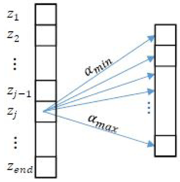
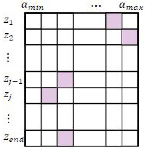
As a simplified illustrative example, Fig. 1 shows a 2D version of C_jklm, i.e., C_jk which considers only one unknown, attenuation coefficient α. We allocate a 2D matrix to store different values of C_jk as z_j and α_k vary (Fig. 2). Every cell in this matrix is filled with cost values at the associated α_k and depth with that cell. In order to find the cost value at a cell in Fig. 2, we first calculate the Δ term in Eq. 13 at z_j and the corresponding α_k. Then, the minimization part in Eq. 13 is performed. The index j — 1 in this term indicates that the cost value at depth j depends on the cost value at the previous depth. In other words, we add the values stored in row Z_j–1 to the regularization term (Eq. 11) and find its minimum. We also store the values of unknown coefficients for which this minimization occurs (a step technically known in DP as memoization). These locations are stored in M, a 2D matrix with the same size as C in this reduced example. Finally, the Δ term added to the minimum value is stored as the value of the cost function at the corresponding cell to be used for the next depth.

Fig. 1.

At each ROI z_j, different values of α_k, b_l, and n_m are explored. To simplify illustration, only α is shown in this figure.

Fig. 2.

2D matrix of cost values at different depths and α_k. Pink cells represent the minimum values that are traced back from the last row to the first one using memoization matrix M. The cost function in this paper is 4D. To simplify illustration, only α is shown in this figure.

The DP cost function must be calculated for every axial row. After that, a final minimization is performed on the cost function in the last row to estimate the α at that depth. Then, starting from the values stored in M, we trace back the minimum points to the first row using the memoization matrix M.

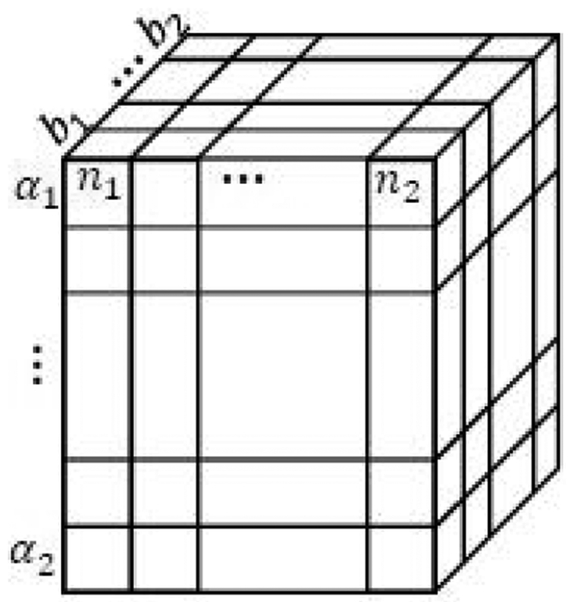
Extending this reduced example of DP to the quantitative ultrasound problem in Eq. 13 with three unknowns, u, and depth dependency, the matrix in Fig. 2 as well as memoization matrix M change to 4D matrices. Consequently, cost values at depth j illustrated as a row in Fig. 2 will be a 3D matrix as shown in Fig. 3.

Fig. 3.

3D matrix of the cost values at one specific depth. It corresponds to one ROI of the 2D matrix in the Fig. 2 wherein only α was considered as an unknown.

C. Data acquisition

1). Homogeneous phantoms:

Two homogeneous tissue-mimicking phantoms, a sample and a reference, were used to compare the performance of the LSq and DP algorithms. The reference phantom consisted of an agarose-based gel with graphite powder within a 15×15×5 cm³ acrylic box [25]. The sample phantom was a mixture of water-based agarose-propylene glycol and filtered milk within a 16×10×10 cm³ acrylic box [25]. Both phantoms had scanning windows covered by a 25 μm thick Saran-Wrap (Dow Chemical, Midland MI, USA). Solid glass beads (5-43μm diameter; Spheriglass 3000E, Potter Industries, Malvern, PA) with a mean concentration of 236 scatterers/mm³ were added to produce incoherent scattering. Ground truth values of each phantom α, b and n (Table I) were measured from 2.5 cm-thick test samples using narrowband substitution (attenuation) and broadband pulse-echo (backscatter) techniques with single-element transducers [26], [27].

TABLE I.

Ground Truth Values for the Uniform Phantom.

	Reference Phantom	Sample Phantom
α (dB/cm-MHz)	0.670	0.654
b (1/cm-sr-MHzn)	8.79e-06	1.02e-06
n	3.14	4.16

Both phantoms were scanned with a 9L4 38 mm-aperture, linear array transducer on a Siemens Acuson S3000 scanner (Siemens Medical. Solutions USA, Inc., Malvern, PA) operated at 6.6 MHz center frequency and a transmit focal depth of 3 cm. The scanner was enabled with the Axius Direct ultrasound research interface to provide radiofrequency (RF) echo data sampled at 40 MHz. [28] Ten statistically independent RF data frames, each separated by at least one elevational aperture, were acquired from each phantom. The following search ranges were used for both LSq and DP:

$$\begin{array}{c}\hfill {\alpha }_s-0.5\le \alpha \le {\alpha }_s+0.5\hfill \\ \hfill e^{-1}{b}_s\le b\le e^1{b}_s\hfill \\ \hfill n_s-2\le n\le n_s+2\hfill \end{array}$$

where α_s, b_s, and n_s are ground truth values of the sample phantom.

2). Layered phantoms:

To compare the performance of the LSq and DP algorithms when estimating piece-wise varying acoustic properties, we applied both methods to RF data from two layered tissue mimicking phantoms, each composed of three axially arranged layers: a 4 cm-thick top layer, a 1.5 cm-thick bottom layer, and a 1.5 cm-thick central layer offering contrast of either attenuation or backscatter with respect to the other two layers. [29] The first phantom had uniform backscatter and higher attenuation in the second layer. The second phantom had uniform attenuation and a central layer with 6 dB higher backscatter than the other two layers. Both phantoms consisted of an emulsion of ultrafiltered milk and water-based gelatin with 5–43 μm diameter glass beads as sources of scattering (3000E, Potters Industries, Valley Forge, Pennsylvania). Attenuation was controlled by varying amounts of evaporated milk, while the strength of backscatter was increased by augmenting the concentration of glass beads. More detail on the phantom properties can be found in Nam et al. [16] Ground truth values of attenuation and backscatter parameters of the three layers were obtained similarly as for the uniform phantoms and are shown in Tables II and III.

TABLE II.

Ground Truth Values for Layered Phantom with Uniform Backscatter.

	Layer 1	Layer 2	Layer 3
α (dB/cm-MHz)	0.510	0.779	0.520
b (1/cm-sr-MHzn)	1.60e-06	3.22e-06	1.60e-06
n	3.52	3.13	3.52

TABLE III.

Ground Truth Values for Layered Phantom with Uniform Attenuation.

	Layer 1	Layer 2	Layer 3
α (dB/cm-MHz)	0.554	0.580	0.554
b (1/cm-sr-MHzn)	4.82e-07	3.94e-06	4.82e-07
n	3.80	3.38	3.80

The layered phantoms were scanned with a 18L6 58 mm-aperture, linear array transducer on a Siemens Acuson S2000 scanner (Siemens Medical. Solutions USA, Inc., Malvern, PA) operated at 8.9 MHz center frequency and a transmit focal depth of 5.3 cm. RF echo data from ten statistically independent RF data frames were obtained through the system’s Axius Direct ultrasound research interface [28].

Reference echo data were obtained from the top layers of the phantoms by scanning from their flank [16]. The search ranges for both DP and LSq for the three parameters of interest included the expected values for each phantom’s layer:

$$\begin{array}{c}\hfill {\alpha }_{\mathit{sMin}}-0.5\le \alpha \le {\alpha }_{\mathit{sMax}}+0.5\hfill \\ \hfill e^{-1}{b}_{\mathit{sMin}}\le b\le e^1{b}_{\mathit{sMax}}\hfill \\ \hfill n_{\mathit{sMin}}-2\le n\le n_{\mathit{sMax}}+2\hfill \end{array}$$

where α_sMin, b_sMin, and n_sMin refer to the minima of the ground truth values in three layers of the layered phantoms for the coefficient α, b, and n, respectively, and α_sMax, b_sMax, and n_sMax correspondingly refer to the maxima of the ground truth values in three layers of the layered phantoms for the coefficient α, b, and n.

D. Data processing

Both LSq and DP were implemented on the RF data frames using custom-built MATLAB routines. Echo-signal power spectra were computed at different axial and lateral locations by raster-scanning a 4×4 mm² spectral estimation window with an 85% overlap ratio and using a multitaper approach with NW=3 [30]. Because different transducers were used in each experiment, this approach produced a power spectrum array with 74 rows and 40 columns for uniform phantoms and 108 rows and 86 columns for layered phantoms, which correspond to different axial and lateral locations, respectively. To reduce correlation between different columns, we selected 4 columns in each phantom separated as far as possible as follows. For the uniform phantom, we selected columns 1, 10, 20 and 40. For the layered phantoms, we picked columns 10, 30, 45, and 80. Each experiment consists of 10 frames, yielding a total of 40 total columns in each experiment. Each cell contained a vector of normalized power spectrum estimates. The LSq and DP estimators were fed with the normalized power spectra in the frequency range from 3.7–7 MHz corresponding to the spectral band with power content at least 10 dB above the noise floor measured at 15 MHz.

We applied DP and LSq to four different lateral positions from 10 different frames of RF data, i.e 40 sample positions in total. The weights of the regularization term in DP for uniform phantom were set to 10⁸ in all 40 sample positions. To provide a fair comparison, we used identical search ranges for both LSq and DP.

In the case of the layered phantoms, the LSq and DP methods were applied to the 108 rows and 40 columns of power spectra from 10 different frames. The weights of the DP regularization were set to w_α = 10⁶ and w_b = w_n = 10³ for the uniform backscatter phantom, and w_α = 5 × 10⁶ and w_b = w_n = 10 for the uniform attenuation phantom. These weights are automatically selected as follows. First, we run LSq and investigate the Normalized Range (NR) of b values by dividing the range of LSq estimations for backscatter coefficient b by the mean value of estimates. If the NR is greater than eight, we use the lower regularization value for w_b and w_n above. Otherwise, these weights are set to a higher value as for the uniform backscatter phantom. This is similar to our previous work on Conditional Random Fields (CRF) [31] where we adjust the regularization term based on the data term.

III. Results

A. Uniform Phantom

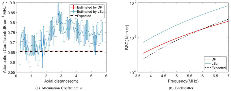
Fig. 4(a) shows the DP (red) and the LSq (blue) estimates of α_s vs axial distance. Thick, colored lines and errorbars correspond to the mean and standard deviations among 40 estimates at each depth, respectively. Fig. 4(b) show the reconstructed BSC parameters b_s and n_s. Black dashed lines indicates expected values. DP substantially outperforms LSq in estimation of all three parameters.

Fig. 4.

LSq and DP estimation in the uniform phantom for (a) attenuation coefficient and (b) backscatter coefficients of Eq. 2.

The bias and standard deviation averaged over the 6cm depth range of α_s, b_s and n_s are shown in Table IV, and the uncertainty in these estimates are shown in Table V. The units for parameters α and b are respectively dB·cm⁻¹MHz⁻¹ and cm⁻¹sr⁻¹MHzⁿ while parameter n has no units. Both the value of bias and variance, as well as their uncertainty, are substantially lower in DP compared to LSq except for the bias of backscatter coefficient n by LSq which is slightly less than DP; however the uncertainty is still lower for DP.

TABLE IV.

The standard deviation (STD) and bias in the Uniform Phantom experiment. The smallest values are highlighted in bold font.

	LSq	DP
Standard Deviation
α (dB/cm-MHz)	0.049	2.236e-16
b (1/cm-sr-MHzn)	9.402e-07	1.706e-21
n	0.410	3.577e-15
Bias
α (dB/cm-MHz)	0.080	0.003
b (1/cm-sr-MHzn)	3.660e-06	3.341e-06
n	0.322	0.820

TABLE V.

Uncertainty in STD and Bias in the Uniform Phantom experiment. The smallest values are highlighted in bold font.

	LSq	DP
Standard Deviation
α (dB/cm-MHz)	0.397	0.031
b (1/cm-sr-MHzn)	6.344e-06	3.648e-06
n	2.221	0.353
Bias
α (dB/cm-MHz)	1.744	0.136
b (1/cm-sr-MHzn)	2.790e-05	1.599e-05
n	9.767	1.549

B. Layered Phantom

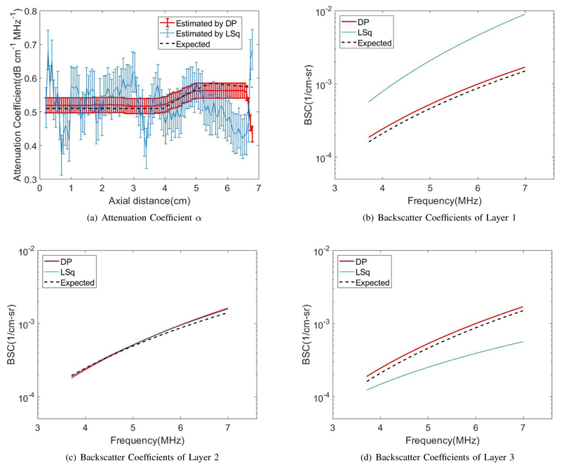
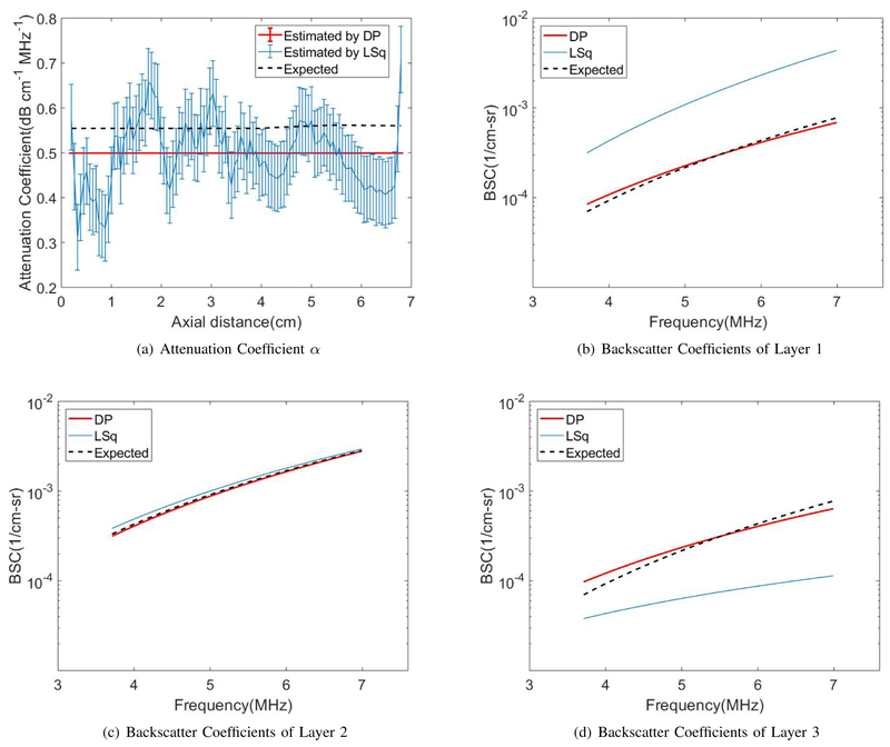
Figs. 5 and 6 show the DP (red) and the LSq (blue) estimates of (a) α_s and (b)-(d) the reconstructed BSC parameters b_s and n_s for each of the three layers vs axial distance. Thick, colored lines and errorbars correspond to the mean and standard deviations among 40 estimates at each depth, respectively. Estimates from the DP method closely follow the depth dependence of effective attenuation α_s, in contrast to the high variance of the LSq method. Black dashed lines indicate expected values. DP substantially outperforms LSq in the estimation of the BSC in each of the three layers.

Fig. 5.

LSq and DP estimation of (a) attenuation coefficients and (b–d) backscatter coefficients of Eq. 2 in the three-layered phantom with uniform backscattering coefficients for layer 1, 2, and 3, respectively.

Fig. 6.

LSq and DP estimation of (a) attenuation coefficient and (b–d) backscatter coefficients of Eq. 2 in the three-layered phantom with uniform attenuation coefficients for layer 1, 2, and 3, respectively.

The standard deviation and bias of the two-layered phantoms, as well as the uncertainties of these measurements, are shown in Tables VI to IX. Again, DP substantially outperforms LSq in terms of both standard deviations of the estimates as well as the uncertainty in these estimates. Although the bias of LSq and DP estimates are comparable, the uncertainty in the estimated bias is substantially lower in DP.

TABLE VI.

The STD and bias in the Layered Phantom with Uniform Backscatter experiment. In each layer, the smallest values are highlighted in bold font.

	Layer 1		Layer 2		Layer 3
	LSq	DP	LSq	DP	LSq	DP
STD
α (dB/cm-MHz)	0.059	0.001	0.038	0.014	0.069	0.035
b (1/cm-sr-MHzn)	8.423e-07	7.132e-09	8.979e-07	1.697e-08	5.774e-06	1.471e-07
n	0.323	0.021	0.400	0.014	0.842	0.081
Bias
α (dB/cm-MHz)	0.022	0.009	0.028	0.004	0.091	0.028
b (1/cm-sr-MHzn)	1.272e-06	3.441e-07	4.155e-07	1.242e-06	5.527e-06	5.036e-07
n	0.117	0.062	0.188	0.320	0.290	0.0139

TABLE IX.

Uncertainties in STD and Bias of Layered Phantom with Uniform Attenuation. In each layer, the smallest values are highlighted in bold font.

	Layer 1		Layer 2		Layer 3
	LSq	DP	LSq	DP	LSq	DP
STD
α (dB/cm-MHz)	0.670	0.156	0.314	0.156	0.237	0.156
b (1/cm-sr-MHzn)	5.006e-06	1.549e-06	1.081e-05	4.788e-06	1.466e-05	1.150e-05
n	3.063	1.056	3.503	1.890	2.883	2.206
Bias
α (dB/cm-MHz)	2.697	0.627	0.800	0.398	0.551	0.365
b (1/cm-sr-MHzn)	1.976e-05	6.208e-06	2.752e-05	1.220e-05	3.368e-05	2.624e-05
n	12.326	4.245	8.929	4.817	6.713	5.147

C. Effects of expected attenuation

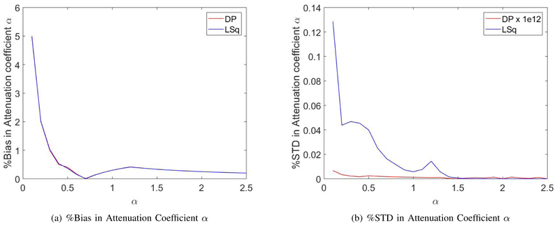
To investigate the performance of DP over a large range of attenuation values, we simulated a new dataset by assigning values of the sample and reference QUS parameters to the log-transformed ratio of power spectra (Eq. 2). Specifically, 0.1 ⩽ α ⩽ 2.5 dB·cm⁻¹MHz⁻¹, and the values of the other parameters were the same as the expected ones for the uniform sample and reference phantoms used in the first experiment. Based on the model developed in Lizzi et al. [32] for the variance of the log-transformed sample-to-reference ratio of power spectra, white noise with variance inversely proportional to the number of independent scanlines used to estimate one power spectrum (N=10) was added to the simulated log-transformed normalized power spectra. DP was run on each of the simulated data sets, and we computed the percent bias and standard deviation of the estimated attenuation with respect to the expected values.

The bias and standard deviation in the results of DP and LSq for different attenuation values are plotted in Fig. 7. As it can be observed in Fig. 7(a), for a higher value of the attenuation coefficient, the bias in the estimation of both methods decreases similarly. However, the standard deviation in the estimation of DP in Fig. 7(b) demonstrates the consistency and substantially smaller standard deviation for all values of α compared to LSq. The standard deviation values of DP are multiplied by 10¹² to be visible in the scale of corresponding values for LSq.

Fig. 7.

Percentage of bias and standard deviation in DP and LSq estimations for simulated data with different attenuation coefficients α.

D. Regularization Weight Analysis

In order to illustrate the impact of regularization weights on the values estimated by DP, we ran the code for a range of regularization weights for the homogeneous phantom to compare the bias (Fig. 8) and standard deviation (Fig. 9) at each weight. The bias and standard deviation of α, b, and n are shown in Figs. 8 and 9, where the corresponding regularization weight is varied from 1 to 10¹⁰ while weights of the other two coefficients were fixed at 10⁸. These results show that increasing the regularization weight has a small effect on bias while substantially reducing the variance.

Fig. 8.

Bias of DP estimations for coefficients α, b, and n at different weight values used in DP. In (a), the regularization weight for b and n are fixed at 1e8 while it varies for α. In (b), the regularization weight for α and n are fixed at 1e8 while it varies for b. In (c), the regularization weight for α and b are fixed at 1e8 while it varies for n.

Fig. 9.

STD of DP estimations for coefficients α, b, and n at different weight values used in DP. In (a), the regularization weight for b and n are fixed at 1e8 while it varies for α. In (b), the regularization weight for α and n are fixed at 1e8 while it varies for b. In (c), the regularization weight for α and b are fixed at 1e8 while it varies for n.

E. DP and LSq Cost Values

In order to observe the functionality of the LSq and DP cost functions at different unknowns along the search ranges we compared them for the layered phantom with uniform backscatter coefficients in Fig. 8. Again, as it is hard to illustrate the 4D cost function, we set α as the only unknown and calculated the cost function of both LSq and DP at their previously estimated values for b and n and different values of α. Fig. 10 compares the averaged cost function values obtained by running LSq and DP for 40 different RF data of this phantom. In Fig. 11, we added n as the second unknown and plotted the 3D cost function with n and α set as variables. These two figures demonstrate that the DP cost function is more convex (i.e. has a higher second order derivative) and is therefore less susceptible to optimization failures.

Fig. 10.

Cost values of DP and LSq at different values of α within the search range in each layer of the phantom with uniform backscattering properties. (a) Layer 1 at the depth of 3.5 cm, (b) Layer 2 at the depth of 4.5 cm, (c) Layer 3 at the depth of 6.5 cm.

Fig. 11.

Cost values of DP and LSq at different values of α and n in each layer of the phantom with uniform backscattering properties. In all three layers, the upper surface is the result by DP. (a) Layer 1 at the depth of 3.5 cm, (b) Layer 2 at the depth of 4.5 cm, (c) Layer 3 at the depth of 6.5 cm.

IV. Discussion

The DP method was introduced to simultaneously estimate attenuation and backscatter coefficients of tissue-mimicking phantoms. DP was selected as the optimization technique because it gives the global minimum of the cost function, and is also computationally efficient. The LSq method, which also simultaneously estimates attenuation and backscatter coefficients, was used as a benchmark. Both methods were tested on three phantoms: one homogeneous phantom and two piecewise homogeneous phantoms.

Fig. 4 clearly indicates that DP results are substantially more precise than Lsq results for both attenuation and backscatter coefficients. The LSq results have a large estimation variance, compared to very small variance in DP results. This large improvement in the performance is due to the inclusion of the regularization term, which acts as a prior information and eliminates noisy data. It is also due to the optimization scheme, wherein DP provides the global minimum of the cost function. Moreover, the bias of DP results in the homogeneous phantom is lower than that of LSq. The exception was the bias of n, which was larger for DP. This bias would affect the bias and precision of estimates of the effective scatterer size, a parameter derived from the frequency dependence of backscatter. We are currently investigating the severity of these effects.

Fig. 5 shows the comparison of the performance of DP and Lsq for the layered phantom with variable attenuation and constant BSC coefficients. Again, as expected, DP estimates have much smaller variance compared to LSq results. We also see that despite the regularization term, DP estimates reproduce more accurately the depth dependence of the three parameters. This is because the penalty for not following the data term at discontinuities overcomes smoothness penalties.

The last experiment which was on the inhomogeneous phantom with constant attenuation and variable BSC coefficients offered interesting results by both LSq and DP (Fig. 6). Although bias averaged over depth was similar between LSq and DP, LSq showed an unexpected trend of decreasing α_s over depth. In addition, the DP results in (b) to (d), demonstrate that BSC parameters estimated by DP are closer to the expected than those estimated by LSq.

The results of Tables IV to IX show the standard deviation and bias of LSq and DP, as well as the uncertainty in these measurements. As expected, DP substantially outperforms LSq in terms of standard deviation of the estimation while giving similar bias. Furthermore, the uncertainty in both standard deviation and bias is substantially lower in the proposed DP method.

Fig. 8 and Fig. 9 show that DP regularization weights have a generally moderate effect on bias and large effect on standard deviation as expected. These weights are often treated as hyperparameters in the machine learning community and have to be adjusted in different applications. Given that ultrasound machines have different imaging presets for imaging different organs (e.g. breast, thyroid, etc.), these hyperparameters can be stored alongside those imaging presets.

As demonstrated by the results, the advantage of the DP method relies on its ability to improve the precision of QUs parameters. In this manuscript, the QUS parameters came from a power-law model of the backscatter coefficient. We chose this model for two reasons. First, this model was assumed in the LSq method, thus facilitating the comparison. Second, the power law does not assume a physical model for the distribution and size of scatterers in the medium. However, Eq. 2 can be considered a particular case of the more general equation:

$$B(f)=B_{0}G(f)$$ (15)

where B₀ and G(f) describe the magnitude and frequency dependence of the backscatter coefficient of tissue, respectively. By properly defining G(f), the DP algorithm can be adapted to quantify different scattering parameters of tissue. For example, G(f) can be defined in terms of scattering form factors to simultaneously estimate attenuation and the effective size of scatterers in tissue, as initially proposed by Bigelow et al. [33]. Under conditions of randomly distributed weak scatters, i.e., diffuse scattering, G(f) takes the form

$$G(f)=f^{4}F(f;a_{\mathit{eff}})$$ (16)

where F(f; a_eff) is the scattering form factor equal to the Fourier transform of the autocovariance function of the scattering field. Under conditions of diffuse scattering, F(f; a_eff) depends only on the effective scatterer size a_eff [34]. Thus, by parameterizing F(f; a_eff), in terms of a mathematical model, such as a Gaussian function or an exponential function, the DP algorithm can be modified to estimate the effective scatter size, as well as parameters related to the magnitude of scattering and the total attenuation. In this sense, this adaptation of the DP algorithm would expand the work of Bigelow et al. [33], [35] by quantifying the backscatter coefficient magnitude (related to the number density and impedance difference of scatterers – relative to the background) and by using regularization and dynamic programing to improve the precision of the estimated parameters. Alternatively, the DP algorithm can be adapted to compute the packing factor and size of aggregates of Rayleigh scatterers, as proposed by Franceschini et al. [36], [37]. In this case, G(z,f) is defined as the product of the Rayleigh backscatter coefficient for individual scatterers (with f⁴ dependence) and the structure factor S(f) which takes into account the interaction of scattering sources. Therefore, the DP strategy can be potentially adapted to quantify parameters from different scattering conditions, improving the precision over previously proposed methods.

We have picked a very large search range to demonstrate that DP provides the correct solution even when no good approximate value is known. When applied to real tissue, based on prior knowledge of the expected values, we can use smaller search ranges that correspond to that tissue, similar to gain settings in imaging presets that current ultrasound machines have for imaging different organs. Since DP running time depends on the search range, this can substantially reduce the computational complexity of DP. For example, if we halve the search range for α, b and n, the running time reduces from 17 hours to 8 hours. Substantially faster runtime can be achieved by implementing the code in C++, parallel implementation of the method, and multi-resolution search [21].

With a look at all results, it is clear that the regularization term substantially reduces the estimation variance as expected. However, the reduction in estimation bias is not as significant as the reduction in variance. This is also expected from the cost function, as the expected value of the parameters slightly changes with the introduction of the regularization term. Bias-variance trade-off is an important issue in estimation theory and an active field of research [38], [39]. We will investigate this trade-off in future work. We are also investigating the performance of the DP algorithm in the presence of specular reflectors that introduce coherent scattering and, therefore, violate the assumption of diffuse scattering behind the derivation of Eq. 6. In addition, we are exploring situations wherein the frequency dependence of scattering is substantially different between reference and sample due to scatterers of different sizes. Moreover, experiments on phantoms with spherical inclusions are a subject of future work.

V. Conclusions

We presented a novel framework for estimation of backscatter quantitative ultrasound parameters based on Dynamic Programming (DP). The new technique incorporates the prior information of depth-continuity of parameters into a cost function that is solved globally using DP. Intuitively, DP considers the data at all depths to estimate u, and finds u that gives the global minimum of the cost function. All values of u at different depths are optimized together in DP, whereas LSq considers each location independently. This substantially reduced the bias and variance in DP estimates compared to LSq in homogeneous phantom.

TABLE VII.

The STD and bias in the Layered Phantom with Uniform Attenuation experiment. In each layer, the smallest values are highlighted in bold font.

	Layer 1		Layer 2		Layer 3
	LSq	DP	LSq	DP	LSq	DP
STD
α (dB/cm-MHz)	0.081	5.037e-16	0.043	2.833e-16	0.067	2.844e-16
b (1/cm-sr-MHzn)	1.123e-06	3.622e-07	1.575e-06	3.336e-07	5.857e-06	4.581e-06
n	0.343	0.084	0.508	0.043	0.820	0.212
Bias
α (dB/cm-MHz)	0.050	0.055	0.050	0.059	0.106	0.061
b (1/cm-sr-MHzn)	1.278e-06	6.677e-07	7.073e-07	8.746e-07	4.521e-06	3.206e-06
n	0.352	0.458	0.175	0.083	1.413	0.828

TABLE VIII.

Uncertainties in STD and Bias of Layered Phantom with Uniform Backscatter. In each layer, the smallest values are highlighted in bold font.

	Layer 1		Layer 2		Layer 3
	LSq	DP	LSq	DP	LSq	DP
STD
α (dB/cm-MHz)	0.750	0.067	0.307	0.054	0.264	0.086
b (1/cm-sr-MHzn)	7.170e-06	1.518e-06	8.701e-06	1.685e-06	1.479e-05	2.259e-06
n	3.095	0.454	3.385	0.490	3.252	0.588
Bias
α (dB/cm-MHz)	3.018	0.269	0.783	0.137	0.616	0.199
b (1/cm-sr-MHzn)	2.877e-05	6.102e-06	2.214e-05	4.286e-06	3.429e-05	5.251e-06
n	12.457	1.826	8.630	1.249	7.585	1.370

Biographies

Zara Vajihi was born in Babol, Iran. She received her B.Sc. degree in electrical engineering from Mazandaran (Noshirvani) University, Babol, Iran. She is now pursuing her M.A.Sc. in electrical and computer engineering at Concordia University, Montreal, Canada. Her research interests include medical image processing, machine learning, and quantitative ultrasound.

Ivan M. Rosado-Mendez was born in Merida, Mexico. He received his B.S. in Engineering Physics in 2006 from the Tecnologico de Monterrey, in Monterrey, Mexico and his M.S. in Medical Physics in 2009 from the Universidad Nacional Autonoma de Mexico, in Mexico City. He received his Ph.D. in Medical Physics from the University of Wisconsin-Madison in 2014. He is currently a Research Associate at the Instituto de Fisica of the Universidad Nacional Autonoma de Mexico. His research interests include quantification of coherent and incoherent ultrasonic scattering for tissue characterization as well as the analysis of tissue viscoelasticity using shear wave elastography.

Timothy J. Hall received his B.A. degree in physics from the University of Michigan Flint in 1983. He received his M.S. and Ph.D. degrees in medical physics from the University of Wisconsin-Madison in 1985 and 1988, respectively. From 1988 to 2002, he was in the Radiology Department at the University of Kansas Medical Center, where he worked on measurements of acoustic scattering in tissues, metrics of observer performance in ultrasound imaging, and developed elasticity imaging methods and phantoms for elasticity imaging. In 2003, he returned to the University of Wisconsin-Madison, where he is a Professor in the Medical Physics Department. He also leads the overall ultrasound effort in the Radiological Society of North America’s (RSNA) Quantitative Imaging Biomarker Alliance (QIBA) that works toward “industrializing” image-based biomarkers. His research interests continue to center on developing new image formation strategies based on acoustic wave propagation and tissue viscoelasticity, the development of methods for system performance evaluation, and quantitative biomarker development.

Hassan Rivaz was born in Tehran, Iran. He received his B.Sc. from Sharif University of Technology, his M.A.Sc. from University of British Columbia, and his Ph.D. from Johns Hopkins University. He did a post-doctoral training at McGill University. He is now an Assistant Professor at the Department of Electrical and Computer Engineering at Concordia University, where he is directing the IMPACT lab: IMage Processing And Characterization of Tissue. He is also a Concordia University Research Chair in Medical Image Analysis. He is an Associate Editor of IEEE TMI, an Area Chair of MICCAI2017 and MICCAI 2018 conferences, a co-organizer of CuRIOUS MICCAI 2018 Challenge on correction of brain shift using ultrasound, and a co-organizer of CereVis MICCAI 2018 challenge on Cerebral Data Visualization.

References

- [1].Feleppa EJ, Machi J, Noritomi T, Tateishi T, Oishi R, Yanagihara E, and Jucha J, “Differentiation of metastatic from benign lymph nodes by spectrum analysis in vitro.” Proc IEEE Ultrason Symp, vol. 2, pp. 1051–0117, 1997. [Google Scholar]
- [2].Rubert N and Varghese T, “Scatterer number density considerations in reference phantom-based attenuation estimation,” Ultrasound in Medicine and Biology, vol. 40, no. 7, pp. 1680–1696, 2014. [DOI] [PMC free article] [PubMed] [Google Scholar]
- [3].Rouyer J, Cueva T, Portal A, Yamamoto T, and Lavarello R, “Attenuation coefficient estimation of the healthy human thyroid in vivo,” Physics Procedia, vol. 70, pp. 1139–1143, 2015. [Google Scholar]
- [4].Anderson CC, Bauer AQ, Holland MR, Pakula M, Laugier P, Bretthorst L, and Miller JG, “Inverse problems in cancellous bone: Estimation of the ultrasonic properties of fast and slow waves using bayesian probability theory,” The Journal of the Acoustical Society of America, vol. 128, no. 5, pp. 2940–2948, 2010. [DOI] [PMC free article] [PubMed] [Google Scholar]
- [5].Nelson AM, Hoffman JJ, Anderson CC, Holland MR, Nagatani Y, Mizuno K, Matsukawa M, and Miller JG, “Determining attenuation properties of interfering fast and slow ultrasonic waves in cancellous bone,” The Journal of the Acoustical Society of America, vol. 130, no. 4, pp. 2233–2240, 2011. [DOI] [PMC free article] [PubMed] [Google Scholar]
- [6].Cai X, Gauthier R, Peralta L, Follet H, Gineyts E, Langer M, Yu B, Olivier C, Peyrin F, Mitton D et al. , “Relationships between cortical bone quality biomarkers: Stiffness, toughness, microstructure, mineralization, cross-links and collagen,” in Ultrasonics Symposium (IUS), 2017 IEEE International. IEEE, 2017, pp. 1–1. [Google Scholar]
- [7].Liu T, Lizzi FL, Silverman RH, and Kutcher GJ, “Ultrasonic tissue characterization using 2-d spectrum analysis and its application in ocular tumor diagnosis.” Med Phys., vol. 31, pp. 1032–1039, 2004. [DOI] [PMC free article] [PubMed] [Google Scholar]
- [8].Golub RM, Parsons RE, Sigel B, Feleppa EJ, Justin J, Zaren HA, Rorke M, Sokil-Melgar J, and Kimitsuki H, “Differentiation of breast tumors by ultrasonic tissue characterization.” Ultrasound Med, vol. 12, pp. 601–608, 1993. [DOI] [PubMed] [Google Scholar]
- [9].Nam K, Zagzebski JA, and Hall TJ, “Quantitative assessment of in vivo breast masses using ultrasound attenuation and backscatter,” Ultrasonic imaging, vol. 35, no. 2, pp. 146–161, 2013. [DOI] [PMC free article] [PubMed] [Google Scholar]
- [10].Nasief HG, Rosado-Mendez IM, Zagzebski JA, and Hall TJ, “Acoustic properties of breast fat,” Journal of Ultrasound in Medicine, vol. 34, no. 11, pp. 2007–2016, 2015. [DOI] [PMC free article] [PubMed] [Google Scholar]
- [11].Parker K, “Scattering and reflection identification in h-scan images,” Physics in Medicine & Biology, vol. 61, no. 12, p. L20, 2016. [DOI] [PubMed] [Google Scholar]
- [12].Ge G, Laimes R, Pinto J, Guerrero J, Chavez H, Salazar C, Lavarello RJ, and Parker KJ, “H-scan analysis of thyroid lesions,” Journal of Medical Imaging, vol. 5, no. 1, p. 013505, 2018. [DOI] [PMC free article] [PubMed] [Google Scholar]
- [13].Insana MF, Hall TJ, Wood JG, and Yan ZY, “Renal ultrasound using para- metric imaging techniques to detect changes in microstructure and function.” Invest Radiol, vol. 28, pp. 720–725, 1993. [DOI] [PubMed] [Google Scholar]
- [14].Oelze ML and Mamou J, “Review of quantitative ultrasound: Envelope statistics and backscatter coefficient imaging and contributions to diagnostic ultrasound,” IEEE Transactions on Ultrasonics, Ferro-electrics, and Frequency Control, vol. 63, pp. 1373–1377, 2016. [DOI] [PMC free article] [PubMed] [Google Scholar]
- [15].Laugier P, Bernard S, Vallet Q, Minonzio J-G, and Grimal Q, “A review of basic to clinical studies of quantitative ultrasound of cortical bone,” The Journal of the Acoustical Society of America, vol. 137, no. 4, pp. 2285–2285, 2015. [Google Scholar]
- [16].Nam K, Zagzebski JA, and Hall TJ, “Simultaneous backscatter and attenuation estimation using a least squares method with constraints,” Ultrasound in medicine & biology, vol. 37, no. 12, pp. 2096–2104, 2011. [DOI] [PMC free article] [PubMed] [Google Scholar]
- [17].Yao LX, Zagzebski JA, and Madsen EL, “Backscatter coefficient measurements using a reference phantom to extract depth-dependent instrumentation factors.” Ultrasound Imaging, vol. 12, pp. 58–70, 1990. [DOI] [PubMed] [Google Scholar]
- [18].Coila A, Anders L, Rpberto J, and Lavarello R, “Regularized spectral log difference technique for ultrasonic attenuation imaging,” IEEE transactions on ultrasonics, ferroelectrics, and frequency control, 2017. [DOI] [PubMed] [Google Scholar]
- [19].Coila AL and Lavarello R, “Regularized spectral log difference technique for ultrasonic attenuation imaging,” IEEE transactions on ultrasonics, ferroelectrics, and frequency control, vol. 65, no. 3, pp. 378–389, 2018. [DOI] [PubMed] [Google Scholar]
- [20].Jiang J and Hall TJ, “A regularized real-time motion tracking algorithm using dynamic programming for ultrasonic strain imaging,” in 2006 IEEE Ultrasonics Symposium, 2006. [Google Scholar]
- [21].Rivaz H, Boctor E, Foroughi E, Zellars R, Fichtinger G, and Hager G, “Ultrasound elastography: a dynamic programming approach,” IEEE Transactions on Medical Imaging, vol. 27, pp. 1373–1377, 2008. [DOI] [PubMed] [Google Scholar]
- [22].Christopher Z, Penate-Sanchez A, and Pham M, “A dynamic programming approach for fast and robust object pose recognition from range images.” IEEE Conference on Computer Vision and Pattern Recognition (CVPR), pp. 196–203, 2015. [Google Scholar]
- [23].Nam K, Rosado-Mendez IM, Rubert NC, Madsen EL, Zagzebski JA, and Hall TJ, “Ultrasound Attenuation Measurements Using a Reference Phantom with Sound Speed Mismatch,” Ultrasonic Imaging, vol. 33, no. 4, pp. 251–263, October 2011. [DOI] [PMC free article] [PubMed] [Google Scholar]
- [24].Jiang J and Hall TJ, “A regularized real-time motion tracking algorithm using dynamic programming for ultrasonic strain imaging,” in Ultrasonics Symposium, 2006. IEEE. IEEE, 2006, pp. 606–609. [Google Scholar]
- [25].Dong F, Madsen EL, MacDonald MC, and Zagzebski JA, “Nonlinearity parameter for tissue-mimicking materials,” Ultrasound in medicine & biology, vol. 25, no. 5, pp. 831–838, 1999. [DOI] [PubMed] [Google Scholar]
- [26].Madsen E, Frank G, Carson P, Edmonds P, Frizzell L, Herman B, Kremkau F, O’Brien W, Parker K, and Robinson R, “Interlaboratory comparison of ultrasonic attenuation and speed measurements.” Journal of ultrasound in medicine, vol. 5, no. 10, pp. 569–576, 1986. [DOI] [PubMed] [Google Scholar]
- [27].Chen JF, Zagzebski JA, and Madsen EL, “Tests of backscatter coefficient measurement using broadband pulses,” IEEE transactions on ultrasonics, ferroelectrics, and frequency control, vol. 40, no. 5, pp. 603–607, 1993. [DOI] [PubMed] [Google Scholar]
- [28].Brunke SS, Insana M, Dahl JJ, Hansen C, Ashfaq M, and Ermert H, “An ultrasound research interface for a clinical system,” vol. 54, no. 1, pp. 198–210, 2007. [DOI] [PubMed] [Google Scholar]
- [29].Nam K, Rosado-Mendez IM, Wirtzfeld LA, Ghoshal G, Pawlicki AD, Madsen EL, Lavarello RJ, Oelze ML, Zagzebski JA, OBrien WD Jr et al. , “Comparison of ultrasound attenuation and backscatter estimates in layered tissue-mimicking phantoms among three clinical scanners,” Ultrasonic imaging, vol. 34, no. 4, pp. 209–221, 2012. [DOI] [PMC free article] [PubMed] [Google Scholar]
- [30].Rosado-Mendez IM, Nam K, Hall TJ, and Zagzebski JA, “Task-oriented comparison of power spectral density estimation methods for quantifying acoustic attenuation in diagnostic ultrasound using a reference phantom method,” Ultrasonic imaging, vol. 35, no. 3, pp. 214–234, 2013. [DOI] [PMC free article] [PubMed] [Google Scholar]
- [31].Karimaghaloo Z, Rivaz H, Arnold D, Collins D, and Arbel T, “Temporal hierarchical adaptive texture crf for automatic detection of gadolinium-enhancing multiple sclerosis lesions in brain mri,” IEEE Trans. Medical Imaging, vol. 34, pp. 1227–1241, 2015. [DOI] [PubMed] [Google Scholar]
- [32].Lizzi FL, Astor M, Feleppa EJ, Shao M, and Kalisz A, “Statistical framework for ultrasonic spectral parameter imaging.” Ultrasound in Medicine & Biology, pp. 1371–1382, 1997. [DOI] [PubMed] [Google Scholar]
- [33].Bigelow TA, Oelze ML, and O’Brien WD, “Estimation of total attenuation and scatterer size from backscattered ultrasound waveforms,” The Journal of the Acoustical Society of America, p. 14311439, 2005. [DOI] [PubMed] [Google Scholar]
- [34].Insana MF and Hall TJ, “Characterising the microstructure of random media using ultrasound,” Physics in Medicine and Biology, vol. 35, no. 10, pp. 1373–1386, 1990. [DOI] [PubMed] [Google Scholar]
- [35].Bigelow TA, Oelze ML, and O’Brien WD, “Signal processing strategies that improve performance and understanding of the quantitative ultrasound spectral fit algorithm,” The Journal of the Acoustical Society of America, p. 18081819, 2005. [DOI] [PubMed] [Google Scholar]
- [36].Franceschini E, Yu FTH, and Cloutier G, “Simultaneous estimation of attenuation and structure parameters of aggregated red blood cells from backscatter measurements,” The Journal of the Acoustical Society of America, no. 123, pp. EL85–EL91, 2008. [DOI] [PMC free article] [PubMed] [Google Scholar]
- [37].Franceschini E, Yu FTH, and Destrempes F, “Ultrasound characterization of red blood cell aggregation with intervening attenuating tissue-mimicking phantoms,” The Journal of the Acoustical Society of America, no. 127, pp. 1104–1115, 2010. [DOI] [PMC free article] [PubMed] [Google Scholar]
- [38].Geman S, Bienenstock E, and Doursat R, “Neural networks and the bias/variance dilemma,” Neural computation, vol. 4, no. 1, pp. 1–58, 1992. [Google Scholar]
- [39].Dekel O, Eldan R, and Koren T, “Bandit smooth convex optimization: Improving the bias-variance tradeoff,” in Advances in Neural Information Processing Systems, 2015, pp. 2926–2934. [Google Scholar]