Abstract
Lung cancer is the leading cause of cancer-related deaths globally, which makes early detection and diagnosis a high priority. Computed tomography (CT) is the method of choice for early detection and diagnosis of lung cancer. Radiomics features extracted from CT-detected lung nodules provide a good platform for early detection, diagnosis, and prognosis. In particular when using low dose CT for lung cancer screening, effective use of radiomics can yield a precise non-invasive approach to nodule tracking. Lately, with the advancement of deep learning, convolutional neural networks (CNN) are also being used to analyze lung nodules. In this study, our own trained CNNs, a pre-trained CNN and radiomics features were used for predictive analysis. Using subsets of participants from the National Lung Screening Trial, we investigated if the prediction of nodule malignancy could be further enhanced by an ensemble of classifiers using different feature sets and learning approaches. We extracted probability predictions from our different models on an unseen test set and combined them to generate better predictions. Ensembles were able to yield increased accuracy and area under the receiver operating characteristic curve (AUC). The best-known AUC of 0.96 and accuracy of 89.45% were obtained, which are significant improvements over the previous best AUC of 0.87 and accuracy of 76.79%.
Keywords: Convolutional Neural Network, CT, Deep Features, Transfer learning, Ensemble, Radiomics, NLST
I. Introduction
With only an 18% 5-year survival rate, lung cancer is one of the leading causes of death around the world and second most cause of cancer-related death in the USA [1]. Early detection is important to diagnose cancer at earlier stages and increase the survival rate for lung cancer. The National Lung Screening Trial (NLST), revealed that cancer mortality was reduced 20% by screening using low dose computed tomography (LDCT) in comparison to standard chest radiography. Based on the NLST study, the USPSTF recommends screening with LDCT once a year for high-risk individuals [31].
Radiomics [2], an approach to extract and analyze quantitative features from radiological images, can be used for early detection and diagnosis of lung nodules. Radiomics features consist of size, shape, location and various texture features extracted from pulmonary nodules.
Deep learning and convolutional neural networks (CNN) are emerging as an alternative approach to analyze lung nodules. Deep CNNs have been very successfully used for the classification of natural camera images and. recently have been applied in chest CT analysis and classification [19–22] on datasets with imaging contrast and tumors while this work focuses on pre-cancerous nodules (images without contrast). Designing and applying a deep CNN with natural camera images is easier because of the availability of large sets of natural images. However, in medical imaging, the availability of data is quite limited for designing a deep CNN. Also, less data can result in an overfit CNN. This problem can be somewhat mitigated using image augmentation to generate more training data. Alternatively, transfer learning can be used, which is a method of applying previously learned knowledge in a new domain. So, a deep CNN trained on a very large dataset of camera images can be applied directly to lung nodules to extract features or the parameters of the pretrained CNN can be tuned with the smaller lung nodule dataset. Another approach is image augmentation (image rotation, flipping, shifting, normalization, etc.) which generates enough images to train a deep CNN from scratch or tune an existing CNN.
Ensemble learning is an approach that combines the predictions of multiple learned models to enhance accuracy. Ensemble prediction using different learning algorithms or different CNN architectures may capture complementary information, which will in turn enable more robust predictions. In this analysis, we used an ensemble approach to predict which lung nodules would become malignant over time. We utilized different types of classifiers, groups of features, and combination methods for ensembles.
We compared our results with our previous published studies. The best AUC obtained from our current study is 0.96, which is a significant improvement over our previous best AUCs of 0.79 [3] using deep features and 0.81 using only quantitative features [4], and 0.87 [3] after training a CNN from scratch. In this study, we obtained the best accuracy of 89.5%, which was a significant improvement over our previous results of 76.8% [3,4].
II. Dataset
In this study, a subset of data from the LDCT-arm of the NLST [14] dataset was used. The NLST study, spanned three years: a baseline scan (T0) followed by two successive scans (T1 and T2) approximately 1 year apart. We selected subsets of participants with lung cancers and nodule positive controls based on prior work by Schabath et al [15]. The subset chosen for our study was divided into two cohorts of subjects: Cohort 1 (85 malignant lung cancer nodules and 176 nodule positive controls) and a separate independent Cohort 2 (85 malignant lung cancer nodules and 152 nodule positive controls). The nodule positive controls had three consecutive nodule positive scans and were not diagnosed with lung cancer through the last follow-up. The lung cancer cases and the nodule positive controls were 1:2 frequency matched on age at randomization, sex, and cigarette smoking history. Cohort 1 was used for training (with augmentation) and the unseen Cohort 2 was used to test. Participants from both cohorts presented with nodules at the baseline T0 screen that were not diagnosed as lung cancer. In the follow-up scan (T1) approximately a year later, in Cohort 1 some participants were diagnosed with lung cancer and some of them remained non-cancer (i.e., nodule positive control). Whereas, in Cohort 2, none of T1 scans were diagnosed as cancer. At T2 (after 2 years of baseline scan T0), some Cohort 2 participants were diagnosed as lung cancer. Figure 1 shows the selection of flowchart of Cohort 1 and Cohort 2.
Fig. 1.
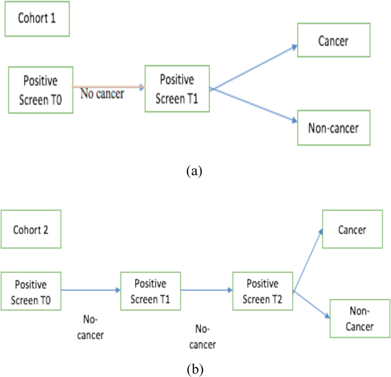
Flowchart of selection of cohort 1 and cohort 2
III. Transfer Learning
Training a CNN typically requires a large amount of data (images here). Hence, transfer learning is a possible solution with a small data set. Transfer learning is a procedure wherein a previously learned model can be applied in another task domain. The domain where learning was done and the domain the knowledge is applied in can be the same or different. In our study, we used the Vgg-s CNN pre-trained on the ImageNet data set [5,6] of 1000 classes of objects in color images. The Vgg-s architecture had five convolutional layers and three fully connected layers. We extracted a deep feature vector of size 4096 from the second fully connected layer after applying the ReLU activation function. The Vgg-s architecture was trained on color images (24 bit, but the pulmonary nodules were grayscale (8 bit). Using information from only one channel (R/G/B) lost the information provided by the other two channels. So, we concatenated the nodule image three times to make it similar in number of bits/channels. Doing so engages all the weights and exploits all the learned knowledge when extracting features from the pre-trained network.
IV. Image augmentation and cnn training
For building an effective CNN, even if it is small, large numbers of images are needed to reduce overfitting. Our dataset had two cohorts from the NLST study: Cohort 1 was used as a training set (261 LDCT screening participants) and the unseen Cohort 2 was used a test set (237 LDCT screening participants). We augmented our training set (Cohort 1) first by rotations of 15 degrees and then flipping the images horizontally and vertically. By doing so, we generated 72 augmented images for each nodule image and 18,792 in total. We used 70% of the augmented images with the original images in training the CNN and the 30% remaining for validation. Three different CNN architectures were designed in Keras [7] using Tensorflow [8] as the backend. The largest nodule size for Cohort 1 cancer cases and control cases were 104×104 pixels, and 82×68 pixels respectively and the smallest nodules for Cohort 1 cancer cases and control cases were 8×10 and 8×8 respectively. So, we chose 100×100 as the input image size for the designed CNN. We trained the CNN for 200 epochs. RMSprop was used as the gradient descent optimization algorithm along with a constant learning rate of 0.0001. A batch size of 16 was used for both training and validation. In convolutional layers 1 and 2, leaky ReLU with an alpha value 0.01 was applied. Doing so permits some negative values to propagate through the convolution layer and provides non-linearity on the convolution layer output. As the classification problem had two classes, binary crossentropy was used as the loss function. Since our designed CNN’s were shallow and small, we used L2 regularization [9] along with dropout [10] to reduce overfitting. While training the CNN, we only monitored the accuracy on the validation data (30% of the augmented data of Cohort 1) and chose the model which produced maximum accuracy on the validation data to test on unseen Cohort 2 data. As deep neural networks are notoriously affected by their many parameters, we designed several small CNN architectures trained on Cohort 1. There were 3 architectures tried with an attempt to progressively minimize the number of weights. While more weights can provide more complex classifiers, with small data they can overfit or simply train poorly, but small networks may not give good accuracy. Hence, we designed 3 CNN architectures.
The CNN architecture 1 (Table 1) had 2 convolution layers and two fully connected layers before the final classification layer. The total parameters were 841,681. CNN architecture 2 (Table 2) had 2 convolution layers, followed by one fully connected layer and one LSTM (Long short term memory) layer before the final classification layer. LSTM is a type of recurrent neural network, which consists of memory to remember for a long or short time and various gates to control the flow of information [23–24]. In CNN architecture 2, we wanted to examine whether the advantage of remembering information using a stateless LSTM had any effect on classification. In [25] a cascaded architecture was proposed for face identification. In the main branch the input image was fed through convolution and pooling layers and in another branch resized input was added in the fully connected layer. Inspired by that architecture, we designed our CNN architecture 3 (Table 3 and Figure 2) which was a cascaded architecture where the left and right branches were concatenated into the same size 10×10 vector. Finally, we used another convolution layer before the final classification layer. Adding image information directly will create more specific information for each case. After merging, another convolution and max pooling layer before the final classification layer maintains the generic information about the image and can provide more features of the image to enable a better classification result. The total parameters were 39,553. The total number of parameters was reduced by 100% in this architecture when compared to the other two architectures.
TABLE 1.
CNN architecture 1
| Layers | Parameter | Total Parameters |
|---|---|---|
| Input Image | 100×100 | 841,681 |
| Conv 1 | 64 X 5 X 5, pad 0, stride 1 | |
| Leaky ReLU 1 | alpha = 0.01 | |
| Max Pool 1 | 3×3, stride 3, pad 0 | |
| Conv 2 | 64 X 2 X 2, pad 0, stride 1 | |
| Leaky ReLU 2 | alpha = 0.01 | |
| Max Pool 2 | 3×3, stride 3, pad 0 | |
| Dropout | 0.1 | |
| Fully connected 1+ relu | 128 | |
| Fully connected 2 + relu | 8 | |
| L2 regularizer | 0.01 | |
| Dropout | 0.25 | |
| Fully connected 3 | 1 sigmoid | |
TABLE 2.
CNN architecture 2
| Layers | Parameter | Total Parameters |
|---|---|---|
| Input Image | 100×100 | 845,033 |
| Conv 1 | 64 X 5 X 5, pad 0, stride 1 | |
| Leaky ReLU 1 | alpha = 0.01 | |
| Max Pool 1 | 3×3, stride 3, pad 0 | |
| Conv 2 | 64 X 2 X 2, pad 0, stride 1 | |
| Leaky ReLU 2 | alpha = 0.01 | |
| Max Pool 2 | 3×3, stride 3, pad 0 | |
| Dropout | 0.1 | |
| Fully connected 1+relu | 128 | |
| LSTM 1 +relu | 8 | |
| L2 regularizer | 0.01 | |
| Dropout | 0.25 | |
| Fully connected 2 | 1 sigmoid | |
TABLE 3.
CNN architecture 3
| Layers | Parameter | Total Parameters |
|---|---|---|
| Left branch: | 39,553 | |
| Input Image | 100×100 | |
| Max Pool 1 | 10×10 | |
| Dropout | 0.1 | |
| Right branch: | ||
| Input Image | 100×100 | |
| Conv 1 | 64 X 5 X 5, pad 0, stride 1 | |
| Leaky ReLU 1 | alpha = 0.01 | |
| Max Pool 2a | 3×3, stride 3, pad 0 | |
| Conv 2 | 64 X 2 X 2, pad 0, stride 1 | |
| Leaky ReLU 2 | alpha = 0.01 | |
| Max Pool 2b | 3×3, stride 3, pad 0 | |
| Dropout | 0.1 | |
|
Concatenate Left Branch + Right Branch (Merge) |
||
| Conv 3+ReLU | 64 X 2 X 2, pad 0, stride 1 | |
| Max Pool 3 | 2×2, stride 2, pad 0 | |
| L2 regularizer | 0.01 | |
| Dropout | 0.1 | |
| Fully connected 1 | 1 sigmoid | |
Fig. 2.

Overview of CNN architecture 3
V. Ensemble approach
Ensemble classification [11–13] is an approach to combine several of the same or different types of learned models into one predictive model to enhance prediction performance. An ensemble model is typically more stable model and less noisy than a single model. Ensembles usually make the predictive model more robust and give better accuracy on test cases. Ensembles reduce variance and sometimes bias. There are a number of approaches to create the final output value from an ensemble e.g. averaging probabilities, voting, median, max, etc. In our study, we used average probability, accumulating votes for the class with the maximum probability from each classifier [26–27] and a median probability to combine predictions. We extracted the prediction from our different models on the test set and combined them to obtain a final prediction.
VI. Experiments
For standard radiomics, nodules were segmented using Definiens® [16] in conjunction with radiologists from Moffitt Cancer Center. We extracted 219 quantitative features (3D) consisting of size, shape, texture and location from the nodules [4] for our radiomics models. Symmetric uncertainty feature selection was applied to extract 5/10/15/20 top ranked features. Feature set sizes were chosen to match previous work where around 20 or less extracted features have been found stable across different acquisitions [4]. The data set used was relatively small and for comparison purposes we selected the same number of features from CNN’s also
After the radiomic features were extracted, random forests classifiers [18] were applied using the selected features for classification. For both transfer learning and training a CNN, we chose the single slice that had the largest nodule area for each patient case. We extracted only the nodule region by putting a rectangular box around the nodule that completely fit the nodule. For transfer learning using Vgg-s the required input image size was 224×224, and the extracted nodule images were of different sizes. So, bi-cubic interpolation was applied on the nodule images. Figure 3 shows one interpolated nodule along with the lung slice with nodule outlined. We extracted a 4096-feature vector from the pre-trained network (taking the outputs of the last fully connected layer before the output layer) and applied symmetric uncertainty [17] feature selection to extract 5/10/15/20 top ranked features. The random forests classifiers [18] used the selected features for classification.
Fig. 3.
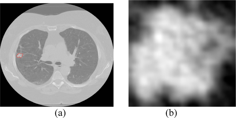
(a) lung image with nodule inside outlined by red (b) extracted nodule (nodule pixel size= 0.625 mm)
For training our CNN’s, extracted nodule images were interpolated to an image size of 100×100 and the sigmoid layer was used for classification.
VII. Results
This section contains an analysis of the results obtained using different classifiers and the ensemble of classifiers approach. Area under the receiver operator characteristic (ROC) curve and accuracy on the unseen Cohort 2 test data was used for performance evaluation. At different decision thresholds, the true positive rate (Y-axis) is plotted against the false positive rate (X-axis) in an ROC curve, for each decision threshold, the point on the ROC curve illustrates a true positive/false positive pair. How well a model can differentiate the lung cancer cases from the control nodules can be measured using area under the ROC curve or AUC. The AUC value lies between 0 and 1 with values closer to 1 indicating a better predictive model.
The best result obtained using only the quantitative features was 76.79% accuracy (AUC 0.81) [4] from random forests classifiers with the top 10 selected features using relief-f. Our random forest had 200 trees and for n total features used lg(n) to randomly choose features for evaluation at each internal node.
Using the Vgg-s pre-trained CNN, we obtained the best result of 75.1% accuracy (AUC 0.74) from random forests classifiers and 15 features chosen using symmetric uncertainty.
By training our CNN architectures, we obtained the best result of 76% accuracy with 0.87 AUC from Architecture 3 while having over 100% less parameters than CNN architectures 1 and 2. Detailed results using different CNN architectures are shown in Table 4. While training the CNN we choose the model which had the maximum validation accuracy. In Table 4 for each CNN architecture we show the maximum validation accuracy while training and using those models to obtain accuracy and AUC on Cohort 2 (unseen test set). Figure 4 shows some of the intermediate layer outputs from the CNN. Loss and accuracy plots while training CNN architecture 3 are shown in Figure 5. We were tracking the validation accuracy and the maximum validation accuracy of 81% obtained is shown (with green circle) in Figure 5 (a). Figures 6 and 7 show the accuracy and loss graph for CNN architectures 2 and 1 respectively.
TABLE 4.
Results from different CNN architectures
| CNN Architectures | Classification Accuracy On 30% validation data | Classification Accuracy On Cohort 2 | AUC |
|---|---|---|---|
| CNN Architecture 1 | 80% | 75.1% | 0.82 |
| CNN Architecture 2 | 81% | 75.5% | 0.86 |
| CNN Architecture 3 | 81% | 76% | 0.87 |
Fig. 4.
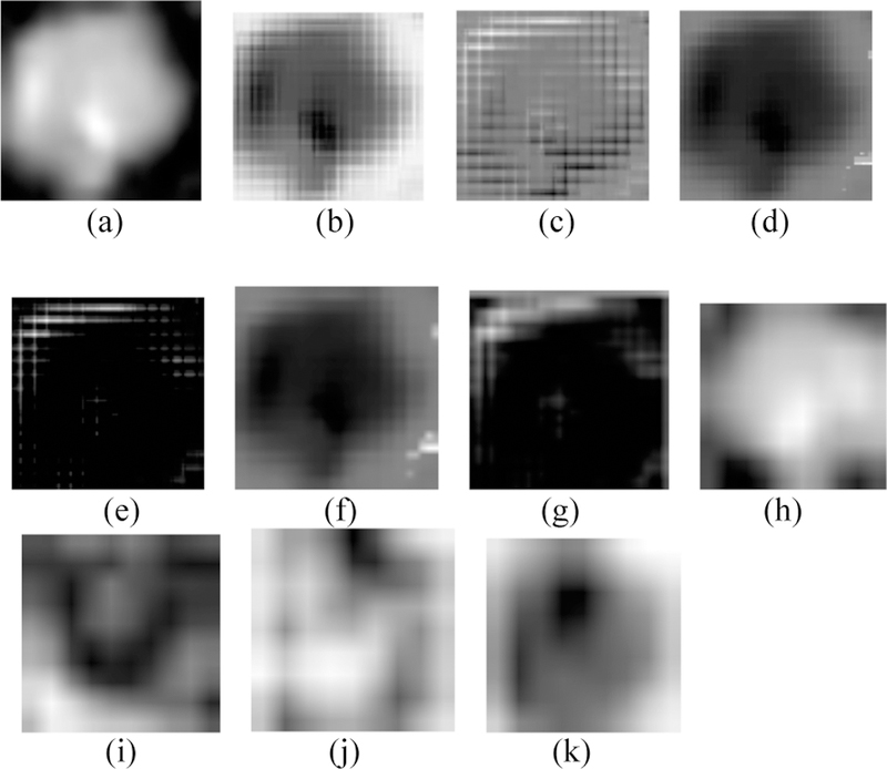
(a) Input 100×100 nodule image, (b, c) Conv 1 layer outputs, (d, e) Leaky ReLU 1 layer outputs, (f, g) Pool 1 layer outputs, (h, i) Merge layer outputs, (j, k) Conv 3 layer outputs
Fig. 5.
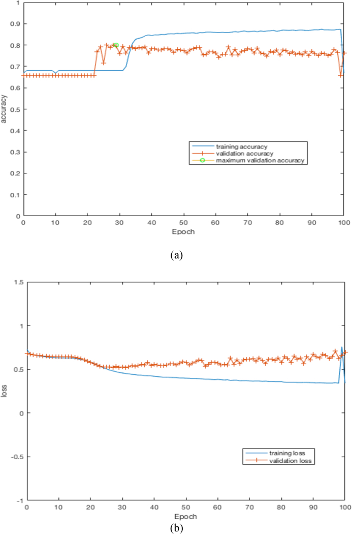
(a) accuracy plot for CNN architecture 3, (b) loss plot for CNN architecture 3
Fig. 6.
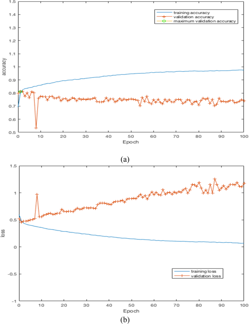
(a) accuracy plot for CNN architecture 2, (b) loss plot for CNN architecture 2
Fig. 7.
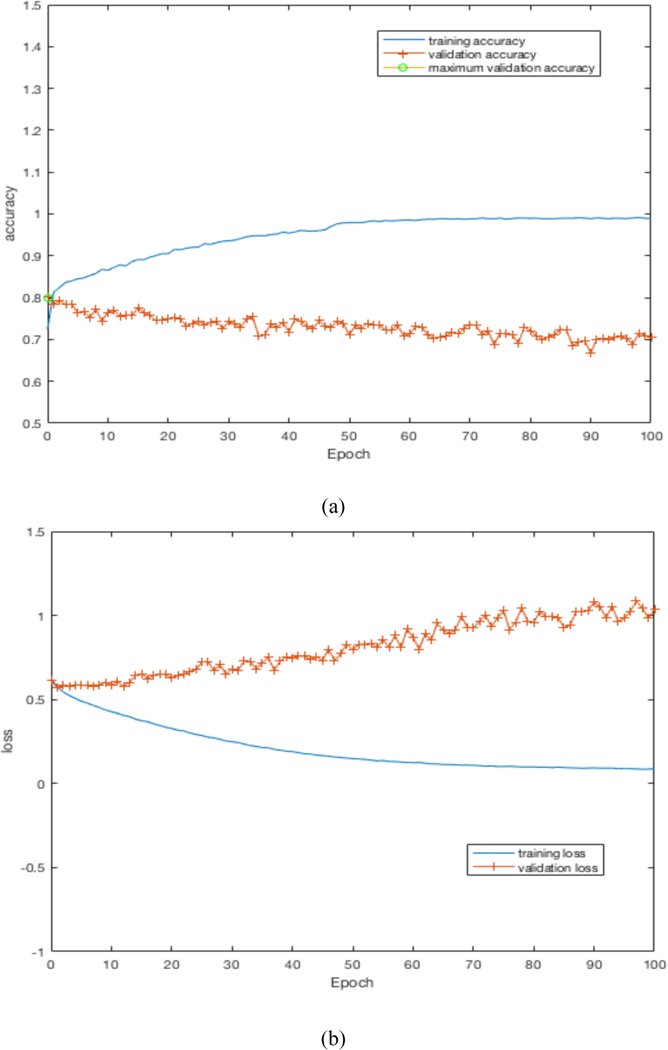
(a) accuracy plot for CNN architecture 1, (b) loss plot for CNN architecture 1
For the ensemble approach, we used three different classifier subsets. The first subset (Subset 1) consisted of only the prediction probability results from the three different CNN architectures. The second subset (Subset 2) had the three best performing models across transfer learning, direct feature extraction and a locally trained CNN. They were the best predictive model using quantitative features (accuracy 76.79%, AUC 0.81), best predictive model using Vgg-s pretrained CNN (75.1% accuracy, AUC 0.74) and the best CNN architecture model (accuracy 76%, AUC 0.87 from CNN architecture 3). The third subset (Subset 3) had 5 models (best quantitative model, best model from a pre-trained CNN and three CNN architecture models trained on lung nodules). For each of these subsets voting (e.g. if two models out of three predict a malignant nodule to be malignant, then classify that nodule as malignant, otherwise classify it benign), the median (extracting the median probability value for each nodule prediction) and averaging (average the probability value for each nodule) were used to create the ensemble prediction. Detailed results are shown in Tables 5–7.
TABLE 5.
Results from an ensemble of 3 CNNs (Subset 1)
| Approach | Average | Median | Voting |
|---|---|---|---|
| Accuracy | 86.91 | 80.16 | 80.16 |
| Accuracy significance (compared with 76.79% from Traditional features) | Significant at p<0.05 | Not Significant at p<0.05 | Not Significant at p<0.05 |
| AUC | 0.94 | 0.91 | 0.77 |
| AUC significance (compared with AUC 0.87 of CNN architecture 3) | Significant at p<0.05 | Not Significant at p<0.05 | NA |
TABLE 7.
Results from ensemble all 5 models (Subset 3)
| Approach | Average | Median | Voting |
|---|---|---|---|
| Accuracy | 89.02 | 84.81 | 89.45 |
| Accuracy significance (compared with 76.79% from traditional features) | Significant at p<0.05 | Significant at p<0.05 | Significant at p<0.05 |
| AUC | 0.96 | 0.94 | 0.85 |
| AUC significance (compared with AUC 0.87 of CNN architecture 3) | Significant at p<0.05 | Significant at p<0.05 | NA |
For subset 1 (ensemble prediction of 3 CNN architecture), in addition to the chosen ensemble approaches (namely, voting, average and median) a sigmoid layer was used to classify the predictions from the 3 architectures. This was done to check whether adding a sigmoid layer could be used to combine the predictions from the ensemble of three CNN’s. Figure 8 shows the ensemble approach by sigmoid layer. Adding a sigmoid layer, we obtained 72.15% accuracy with 0.76 AUC.
Fig. 8.
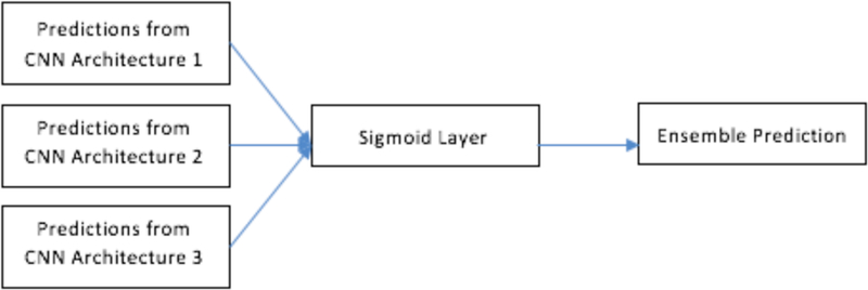
Ensemble of CNN using sigmoid layer.
We analyzed the significance of the AUC and accuracy improvement between the ensemble approaches and the best AUC obtained from single approach (AUC 0.87 from CNN architecture 3) and best accuracy (76.79%) obtained using traditional features and show them in Tables 5–7.
For accuracy significance, the McNemar test was used. For the AUC significance test, the standard error (SE) was computed for each AUC using equation (1).
| (1) |
Where, A is denoted as the calculated AUC, nn and na are the number of cancer and positive controls respectively, and Q1 and Q2 are estimated by,
Using the SE value from two AUC’s e.g., AUC1 and AUC2, the z value was calculated as,
| (2) |
P-value was calculated from the z-value and the calculated p value was checked for significance at p=0.05 (two tailed).
The best results were statistically significantly better with the average probability from an ensemble of 3 CNN’s providing the best combination of accuracy and AUC at 86.91% and 0.94 respectively. From an ensemble of 5 models (3 CNNs, radiomics and transfer learning model) a best accuracy of 89.45% was obtained using voting, whereas the best AUC of 0.96 was obtained by combining via averaging. The accuracy of the average combination approach (89.02%) is statistically indistinguishable from combining by voting.
VIII. Conclusions
In this work, we showed that an ensemble approach significantly enhances the ability to predict lung nodules that will become malignant over time. For the ensembles, we chose three different classifier/feature subsets. Quantitative features consisted of size, shape and texture information about pulmonary nodules in the lung. A CNN pre-trained on natural camera images, Vgg-s, had features extracted for building a classifier. Our CNN architectures were trained on augmented Cohort 1 of our dataset, but each of the architectures has different parameters and different layers. As a result, we have five different models to use in an ensemble approach. Ensemble models that make different predictions from one another will ensure more predictive power than using a single model. We developed three subsets of models: subset 1 had only the 3 designed CNN architectures; subset 2 had the best quantitative model, best designed CNN model and best pretrained Vgg-s model; subset 3 used all 5 models. Ensemble predictions from 3 CNN (subset 1) using a sigmoid layer gave 72.15 accuracy. Combining the ensemble output by averaging yielded the best accuracy and AUC for subset 1 and subset 2 and only the best AUC for subset 3, which was the best AUC obtained. Whereas voting yielded the best accuracy of 89.45% for subset 3, the best results of 0.96 AUC were obtained from subset 3 by the averaging combination approach. The AUC and accuracy were both a statistically significant improvement over the previous best obtained AUC of 0.87 using CNN architecture 3 alone and accuracy of 76.79% by using traditional features.
TABLE 6.
Results from an ensemble of the 3 best models (Subset 2)
| Approach | Average | Median | Voting |
|---|---|---|---|
| Accuracy | 83.96 | 82.57 | 83.54 |
| Accuracy significance (compared with 76.79% from traditional features) | Significant at p<0.05 | Significant at p<0.05 | Significant at p<0.05 |
| AUC | 0.93 | 0.91 | 0.8 |
| AUC significance (compared with AUC 0.87 of CNN architecture 3) | Significant at p<0.05 | Not Significant at p<0.05 | NA |
ACKNOWLEDGMENTS
This research partially supported by the National Institute of Health under grants (NIH U01 CA143062), (NIH U24 CA180927) and (NIH U01 CA200464), National Science Foundation under award number 1513126, by the State of Florida Dept. of Health under grant (4KB17) and DARPA’s SocialSim program under award number FA8650-17-C-7725.
References
- [1].Siegel RL, Miller KD and Jemal A: Cancer statistics, 2016. CA: a cancer journal for clinicians, 66(1), pp.7–30. (2016) [DOI] [PubMed] [Google Scholar]
- [2].Kumar V, Gu Y, Basu S, Berglund A, Eschrich SA, Schabath MB, Forster K, Aerts HJ, Dekker A, Fenstermacher D and Goldgof DB: Radiomics: the process and the challenges. Magnetic resonance imaging, 30(9), pp.1234–1248. (2012) [DOI] [PMC free article] [PubMed] [Google Scholar]
- [3].Paul R, Hawkins SH, Schabath MB, Gillies RJ, Hall LO and Goldgof DB: Predicting malignant nodules by fusing deep features with classical radiomics features. Journal of Medical Imaging, 5(1), p.011021 (2018) [DOI] [PMC free article] [PubMed] [Google Scholar]
- [4].Hawkins S, Wang H, Liu Y, Garcia A, Stringfield O, Krewer H, Li Q, Cherezov D, Gatenby RA, Balagurunathan Y and Goldgof D: Predicting malignant nodules from screening CT scans. Journal of Thoracic Oncology, 11(12), pp.2120–2128. (2016) [DOI] [PMC free article] [PubMed] [Google Scholar]
- [5].Chatfield K, Simonyan K, Vedaldi A and Zisserman A: Return of the devil in the details: Delving deep into convolutional nets. arXiv preprint arXiv:1405.3531 (2014)
- [6].Deng J, Dong W, Socher R, Li LJ, Li K and Fei-Fei L: Imagenet: A large-scale hierarchical image database. In Computer Vision and Pattern Recognition, 2009. CVPR 2009. IEEE Conference on (pp. 248–255). IEEE; (2009) [Google Scholar]
- [7].Chollet F: 2017. Keras (2015).
- [8].Abadi M, Agarwal A, Barham P, Brevdo E, Chen Z, Citro C, Corrado GS, Davis A, Dean J, Devin M and Ghemawat S: Tensorflow: Large-scale machine learning on heterogeneous distributed systems. arXiv preprint arXiv:1603.04467 (2016)
- [9].Ng AY: Feature selection, L 1 vs. L 2 regularization, and rotational invariance. In Proceedings of the twenty-first international conference on Machine learning, p. 78 ACM; (2004) [Google Scholar]
- [10].Srivastava N, Hinton G, Krizhevsky A, Sutskever I and Salakhutdinov R: Dropout: A simple way to prevent neural networks from overfitting. The Journal of Machine Learning Research, 15(1), pp.1929–1958. (2014) [Google Scholar]
- [11].Silva VF, Barbosa RM, Vieira PM and Lima CS: Ensemble learning based classification for BCI applications. In Bioengineering (ENBENG), 2017 IEEE 5th Portuguese Meeting on, pp. 1–4. IEEE; (2017) [Google Scholar]
- [12].Ju C, Bibaut A and van der Laan M: The relative performance of ensemble methods with deep convolutional neural networks for image classification. Journal of Applied Statistics, pp.1–19. (2018) [DOI] [PMC free article] [PubMed]
- [13].Hinton G, Vinyals O and Dean J: Distilling the knowledge in a neural network. arXiv preprint arXiv:1503.02531 (2015)
- [14].National Lung Screening Trial Research Team.: Reduced lung-cancer mortality with low-dose computed tomographic screening. New England Journal of Medicine, 365(5), pp.395–409. (2011) [DOI] [PMC free article] [PubMed] [Google Scholar]
- [15].Schabath MB, Massion PP, Thompson ZJ, Eschrich SA, Balagurunathan Y, Goldof D, Aberle DR and Gillies RJ: Differences in patient outcomes of prevalence, interval, and screendetected lung cancers in the CT arm of the National Lung Screening Trial. PloS one, 11(8), p.e0159880 (2016) [DOI] [PMC free article] [PubMed] [Google Scholar]
- [16].User Guide.: Definiens AG; Germany: Definiens developer XD 2.0.4; (2009) [Google Scholar]
- [17].Yu L and Liu H: Feature selection for high-dimensional data: A fast correlation-based filter solution. In Proceedings of the 20th international conference on machine learning (ICML-03), pp. 856–863. (2003) [Google Scholar]
- [18].Ho TK: Random decision forests. In Document analysis and recognition, 1995., proceedings of the third international conference on, 1, pp. 278–282. IEEE; (1995) [Google Scholar]
- [19].Hussein S, Gillies R, Cao K, Song Q and Bagci U: Tumornet: Lung nodule characterization using multi-view convolutional neural network with gaussian process. In Biomedical Imaging (ISBI 2017), 2017 IEEE 14th International Symposium on, pp. 1007–1010. IEEE; (2017) [Google Scholar]
- [20].Song Q, Zhao L, Luo X and Dou X: Using Deep Learning for Classification of Lung Nodules on Computed Tomography Images. Journal of healthcare engineering (2017) [DOI] [PMC free article] [PubMed] [Google Scholar]
- [21].Jiang H, Ma H, Qian W, Wei G, Zhao X and Gao M: A novel pixel value space statistics map of the pulmonary nodule for classification in computerized tomography images. In Engineering in Medicine and Biology Society (EMBC), 2017 39th Annual International Conference of the IEEE (pp. 556–559). IEEE; (2017) [DOI] [PubMed] [Google Scholar]
- [22].Yang H, Yu H and Wang G: Deep learning for the classification of lung nodules. arXiv preprint arXiv:1611.06651 (2016)
- [23].Pesce E, Ypsilantis PP, Withey S, Bakewell R, Goh V and Montana G: Learning to detect chest radiographs containing lung nodules using visual attention networks. arXiv preprint arXiv:1712.00996 (2017) [DOI] [PubMed]
- [24].Gers FA, Schmidhuber J and Cummins F: Learning to forget: Continual prediction with LSTM (1999) [DOI] [PubMed]
- [25].Li H, Lin Z, Shen X, Brandt J and Hua G: A convolutional neural network cascade for face detection. In Proceedings of the IEEE Conference on Computer Vision and Pattern Recognition, pp. 5325–5334. (2015) [Google Scholar]
- [26].Duin RP: The combining classifier: to train or not to train?. In Pattern Recognition, 2002. Proceedings. 16th International Conference on, pp. 765–770. IEEE; (2002) [Google Scholar]
- [27].Zhang CX and Duin RP: An experimental study of one-and twolevel classifier fusion for different sample sizes. Pattern Recognition Letters, 32(14), pp.1756–1767. (2011) [Google Scholar]
- [28].Tieleman T and Hinton G: Lecture 6.5-rmsprop: Divide the gradient by a running average of its recent magnitude. COURSERA: Neural networks for machine learning, 4(2), pp.26–31. (2012) [Google Scholar]
- [29].Hajian-Tilaki K: Receiver operating characteristic (ROC) curve analysis for medical diagnostic test evaluation. Caspian journal of internal medicine, 4(2), p.627 (2013) [PMC free article] [PubMed] [Google Scholar]
- [30].Hanley JA and McNeil BJ: The meaning and use of the area under a receiver operating characteristic (ROC) curve. Radiology, 143(1), pp.2936 (1982) [DOI] [PubMed] [Google Scholar]
- [31].Moyer VA: Screening for lung cancer: US Preventive Services Task Force recommendation statement. Annals of internal medicine, 160(5), pp.330–338. (2014) [DOI] [PubMed] [Google Scholar]


