Educational policy and intergenerational mobility

Abstract

In the United States, there is considerable variation in intergenerational mobility across states. We argue that the distribution of public school spending across school districts under public school finance systems affects intergenerational mobility within the United States. We build a dynamic model in which school districts vote over public school spending per pupil taking the finance system as given. We embed this model with median voting at the district level within a fairly standard model of human capital accumulation. Our model can replicate the relationship between the distribution of public school spending and intergenerational mobility observed in data. Furthermore, three counterfactual simulations suggest that i) the correlation between parental human capital and a child’s learning ability plays a significant role in explaining the cross-state variation in intergenerational mobility, ii) a more equal distribution of public school spending under a foundation program by relaxing a borrowing constraint improves intergenerational mobility, especially when a child’s learning ability is not highly dependent on parental human capital, and iii) switching to a full state funding program improves intergenerational mobility, but not enormously. This is because full state funding limits public school spending, which hinders intergenerational mobility.

1. Introduction

Intergenerational mobility is an important issue in the United States. Evidence suggests that the United States is one of the least mobile countries in the world.² There is also considerable variation in intergenerational mobility at the state level. According to our calculations based on data from Chetty et al. (2014), the most and least mobile states are Hawaii and Mississippi, respectively. In Hawaii, rank–rank slope, a measure of relative mobility, is 0.236, whereas the corresponding value in Mississippi is 0.414. These slopes mean that if the difference in income ranks of two parents is 100, the difference in their child’s income rank will fall to 24 in Hawaii and 41 in Mississippi. Therefore, where a family resides affects a child’s future outcomes significantly.

A natural question is: what factors generate this variation across states? Chetty et al. (2014) argue that segregation, income inequality, school quality, social capital and family structure are highly correlated with the variation in intergenerational mobility. However, since all of these variables are endogenous, more work is needed to better understand the underlying causal factors.

We take the stand that public school spending is an important determinant of intergenerational mobility. Recent evidence suggests that early childhood investments are critical in improving child’s status and consequently, intergenerational mobility (Cunha and Heckman, 2007, and Caucutt and Lochner, 2012). Therefore, spending on public schools potentially plays an important role.

The focus of our paper is on the distribution of public school spending across school districts within a state, which, in practice, is measured as the estimated coefficient of school district income on public schooling spending per pupil (henceforth, the ‘slope coefficient’).³ We find a substantial variation in the distribution of public school spending across states. For example, rich school districts in Illinois tend to spend more on public schools than poor school districts, whereas public school spending is more equally distributed in California. More importantly, we find a positive correlation between the distribution of public school spending and rank–rank slope across states. That is, a more equal distribution of public school spending is associated with lower rank–rank slope. This suggests that the cross-state variation in the distribution of public school spending is a potential contributor to the variation in intergenerational mobility.

We explore the relation between public school spending and intergenerational mobility by taking into account the public school finance systems. In the U.S., there are four public school finance systems: a flat grant program, a full state funding program, a foundation program, and an equalization program. We model a foundation program, the most popular one, and a full state funding program, the ideal one if the goal is to reduce inequality in public school spending. A full state funding program is ideal in terms of equal spending because public school spending is financed only by statewide taxes and local governments cannot impose taxes for additional spending. In contrast, in a foundation program, a minimum amount of public school spending is guaranteed in all school districts by the state government, but local governments can raise spending through a local tax. A foundation program was employed in 39 states in the early 1990s, the period we consider in this paper. Revisiting the relation between public school spending and rank–rank slope by school finance system, we find two salient patterns in data: (1) Among states using a foundation program, there is considerable variation in both the distribution of public school spending and rank–rank slope, and a positive correlation between them still holds; (2) Relative to states with a foundation program, states with a full state funding program have a more equal distribution of public school spending and lower rank–rank slope.

We model the connection between public school spending and intergenerational mobility by extending the framework in Fernandez and Rogerson (2003). In particular, we extend their static model to a dynamic setting with three periods where a child can accumulate human capital both in school and at work. More importantly, human capital accumulation in school depends not only on public resources from the state and local government, but also on private resources from parents and a child’s own learning ability. Public school spending from the state government is determined through majority voting under either a foundation program or a full state funding program. Furthermore, parents can make a non-negative transfer to their children when the children become independent after schooling.

We estimate the model state by state using various data sets. In the estimation, we assume that a child’s own learning ability is correlated with parental human capital. Our estimated model fits some aspects of the data reasonably well. In particular, our model generates a positive correlation between the distribution of public school spending and intergenerational mobility across states. However, the set of targeted states is limited in our estimation highlighting a failure of our model. We drop the states in which the slope coefficient is negative. In our model, in order to generate a negative slope coefficient, the correlation between parental human capital and a child’s learning ability needs to be negative. This leads to a negative rank–rank slope which is inconsistent with data.⁴ With the estimated model, we conduct three counterfactual simulations to understand the determinants of intergenerational mobility. The first simulation shows that the correlation between parental human capital and a child’s learning ability plays an important role in explaining intergenerational mobility. The second simulation shows that allowing parents to borrow against their children’s future income and using it to invest in their children leads to a more equal distribution of public school spending. The effect on rank–rank slope, however, depends negatively on the correlation between parental human capital and a child’s learning ability. With a smaller correlation, allowing parents to borrow against their children’s future income improves intergenerational mobility significantly. In the third simulation, we find that switching to a full state funding program also improves intergenerational mobility. However, when we compare results on rank–rank slope across simulations, we find that the degree to which intergenerational mobility improves in a full state funding program is not dramatic. This result arises from two competing forces prevalent in a full state funding program. On the one hand, a full state funding program leads to a uniform distribution of public school spending across school districts. On the other hand, it restricts the level of public spending. Therefore, poor and middle-income school districts gain little benefit by full state funding. In our exercise, the restriction on public school spending impedes intergenerational mobility in a full state funding program.

To the best of our knowledge, we are the first to model the effect of the distribution of public school spending on intergenerational mobility within a country taking a structural approach. There is now an extensive literature on intergenerational mobility (e.g., Becker and Tomes 1979, 1986; Solon, 1992; Restuccia and Urrutia, 2004; Mazumder, 2005, and Lee and Seshadri, 2014), but these papers consider income mobility of the U.S. at the aggregate level.⁵ Another strand of literature compares mobility across countries (Corak, 2013; Holter, 2015, and Abbott and Gallipoli, 2014). Chetty et al. (2014) offer a first look at intergenerational mobility at a finer division (county level) and propose possible explanations. There is also a large literature on public spending on primary and secondary education. The effect of school finance reform on equality of spending across districts has been discussed extensively. Hoxby (2001) and Card and Payne (2002) examine the short-run effect of school finance equalization using drop-out rates (Hoxby, 2001), and SAT scores (Card and Payne, 2002). Some recent papers discuss the long-run impact of educational reform. For example, Jackson et al. (2016) explore the impact on educational attainment and earnings. Biasi (2015) is the most relevant paper. She studies the consequence of educational reform on intergenerational income mobility. Our approach allows us to obtain a better understanding of the mechanisms at work. Using structural models and a political economy approach, Fernandez and Rogerson (1999), (2003), and Ferreyra (2009) evaluate different funding formulae in terms of the level of educational spending. Different from these papers, we present a dynamic model in order to understand the relationship between educational policy and intergenerational mobility.

The rest of the paper proceeds as follows. Section 2 discusses stylized facts on intergenerational mobility and public school spending across states. In section 3, we describe the model. Section 4 summarizes the estimation method. Section 5 presents the baseline results. Section 6 discusses the counterfactual simulations. Finally, we conclude the paper in Section 7.

2. Facts

This section presents some empirical facts on intergenerational mobility and educational policy in the U.S.

2.1. Intergenerational mobility

We use rank–rank slope as a measure of intergenerational mobility. Rank–Rank slope measures the association between parent income rank and their children’s income rank as adults. A higher rank–rank slope indicates a larger dependence of child income on parent income and a lower intergenerational mobility. Relative to other measures like the intergenerational income elasticity (IGE), rank–rank slope is more robust to factors like the presence of low- or zero-income observations.⁶ We calculate rank–rank slope for each state as the weighted average of the county level estimates in Chetty et al. (2014),⁷ where the weight for each county is its population from the 2000 census.

Table 1 reports states with the lowest and highest rank–rank slope. Hawaii has the lowest rank–rank slope, with a value of 0.236. It suggests that the difference in income rank between two children, one born to the richest parents and the other born to the poorest parents in Hawaii, is only about 23.6. In contrast, if the two children were born to the richest and poorest parents in Mississippi, the state with the highest rank–rank slope, the difference in their income ranks will be 41.4. Clearly, there is substantial variation in intergenerational mobility across states, and place of residence while young affects future outcomes significantly.

Table 1.

States with the lowest and highest rank–rank slope.

	State	Rank–Rank slope		State	Rank–Rank slope
1st	Hawaii	0.236	51st	Mississippi	0.414
2nd	California	0.237	50th	Louisiana	0.395
3rd	Utah	0.244	49th	Delaware	0.394
4th	Idaho	0.245	48th	Ohio	0.392
5th	Wyoming	0.254	47th	Alabama	0.390

2.2. Public school spending

One potential explanation for the cross-state variation in intergenerational mobility is differences in public school spending. If one state spends more on the education of children born to poor parents than another, other things equal, we should expect a higher intergenerational mobility and a lower rank–rank slope. To provide some evidence, we calculate public schooling spending per pupil and median household income for each school district in each state. This allows us to examine whether children in poor school districts benefit more from public school spending or not.

Using the public elementary and secondary education finance data from the U.S. Census Bureau, we calculate public schooling spending per pupil for each school district in each year by dividing total spending by the number of students.⁸ Because we are going to relate public school spending to rank–rank slope reported earlier, and rank–rank slope in Chetty et al. (2014) are calculated for individuals born in 1980–1982, we use CPI to adjust the spending in each year and calculate a measure of average public school spending per pupil between 1990 and 1998 for each school district. As a proxy for the income level of a school district, we use median household income obtained from the 2000 school district tabulation of the National Center for Education Statistics.

For each state, we run a regression of average public school spending on median household income across school districts. We use the slope coefficient as a measure of the distribution of public school spending across school districts in a state. The distribution of public school spending varies substantially across states, even among states with similar characteristics. For example, California and Illinois have nearly the same number of school districts (989 for California vs 897 for Illinois), and average public school spending per pupil at the state level is also very similar in the two states ($5,472 in California vs $5,360 in Illinois). However, as Fig. 1 shows, the distribution of public schooling spending is very different between these states. There is the negative but insignificant slope coefficient in California, while the slope coefficient in Illinois is positive and statistically significant at the 1% significance level. This suggests that, relative to California, public school spending in Illinois tends to favor children born to richer parents. Other things equal, this difference could result in a lower intergenerational mobility in Illinois than in California. Consistent with this argument, rank–rank slope is higher in Illinois (0.369) than in California (0.237).

Fig. 1.

Public school spending per pupil and median household income across school districts.

Fig. 2 plots the distribution of public school spending measured by the slope coefficient and rank–rank slope across states.⁹ States marked with a solid dot are those for whom the estimated the slope coefficient is statistically significant at 5% significance level. Evidently, there is considerable variation in the slope coefficient across states. The slope coefficient is negative in some states, indicating a negative correlation between median household income and public school spending across school districts. Some of the negative coefficients, however, are statistically insignificant. According to our estimation, 20 states have statistically significant negative slope coefficients. More importantly, there is a positive correlation between our measure of the distribution of public school spending and rank–rank slope. Evidence in Fig. 2 is consistent with the idea that more educational spending on richer children reduces intergenerational mobility. Clearly, we should take the distribution of public school spending into consideration in order to understand intergenerational mobility in the U.S.

Fig. 2.

Distribution of public school spending and rank–rank slope across states.

2.3. Public school finance systems

One important determinant of the distribution of public school spending in a state is the school finance system. According to the American Education Finance Association (1992, 1995), there are four school finance systems: a flat grant program, a full state funding program, a foundation program, and an equalization program. In this paper, we focus on a foundation program and a full state funding program.

We model a foundation program because it is the most popular program in the U.S. For example, 37 states in 1990–1991 and 39 states in 1993–1994 employed this finance system.¹⁰ In a foundation program,¹¹ the state government sets a minimum amount of public school spending guaranteed for all school districts, and local governments are allowed to levy taxes to increase their public school spending. This is different from a full state funding system where all public school spending is financed by statewide taxes, and local governments cannot impose taxes to raise spending on their public schools. A full state funding system was used in California, Hawaii and Washington.¹² We consider this system because it is the ideal system if the goal is to equalize public school spending across school districts within a state.

Fig. 3 plots our measure of the distribution of public school spending and rank–rank slope for states using the two finance systems. States marked with either a solid dot or an X employ a foundation program, while other states adopt a full state funding program. Additionally, either a solid dot or a triangle have an estimated slope coefficient that is statistically significant at the 5% level. Two salient features can be seen from the figure. First, there is considerable variation in both the distribution of public school spending and rank–rank slope among states using the foundation program. Secondly, rank–rank slope is much lower in states employing a full state funding system (California and Washington), likely because public school spending is more equally distributed in these states.¹³

Fig. 3.

Public school spending and rank–rank slope by finance system.

3. Model

We present a model to capture the relationship between public school spending and intergenerational mobility presented in the previous section. Our model is an extension of Fernandez and Rogerson (2003) who explore the implications of public school finance systems in the U.S.

3.1. Model environment

We consider a three-period model economy. The first period is 18 years, and the last two periods are 6 years each. We keep track of each child from birth until the age of 30. There is a continuum of individuals whose population is normalized to be one. In each state, there are n school districts. The income of parents in school district j(∈{1, 2, ..., n}) is denoted by y_j. For simplicity, we assume there is no income heterogeneity within a school district, and assume that the distribution of parental income y_j across school districts in a state is exogenous.

In the first period, parents in each school district j invest in their children, choose their consumption c_j1, and leave the rest of their income g_j as a transfer to their children who can use these resources in the second period. They do so to maximize their utility given by

$$u(C_{j1})+\theta V(a_j,h_{j2},g_j),$$

where u(c_j1) is the utility from consumption, V (a_j, h_j2, g_j) is the lifetime utility of their children starting from the second period which is specified in more detail later, and θ is a measure of parental altruism.

We assume all children attend public schools in the school district where they were born. We also assume that g_j ≥ 0 so that parents cannot leave debt to their children. This is an important friction in the model. It leads to intergenerationally constrained and unconstrained families and hence a role for government intervention to improve allocative efficiency.

Different from Fernandez and Rogerson (2003) who only consider the quantity of a child’s education from public resources, we allow the amount of human capital that a child can accumulate in the first period to depend on (1) public resources, (2) private inputs, and (3) a child’s learning ability. Specifically, for children in school district j, the stock of human capital at the beginning of the second period, h_j2, is given by

$$h_{j2}=a_j{[\omega {\chi }_{j1}^{\varphi }+(1-\omega ){\stackrel{‒}{\chi }}_j^{\varphi }]}^{\frac{\gamma }{\varphi }},$$ (1)

where a_j is a learning ability, χ_j1 and ${\stackrel{‒}{\chi }}_j$ represent private and public inputs, respectively, ω is the share of private inputs, φ is the elasticity of substitution between private and public inputs, and γ is a measure of returns to scale.

Children become independent at the beginning of the second period. They make decisions on human capital accumulation and consumption in the second and third period to maximize utility

$$V(a_j,h_{j2},g_j)=\underset{\{c_{j2},c_{j3},n_{j2},{\chi }_{j2}\}}{\max }u(c_{j2})+\beta u(c_{j3})$$

subject to the budget constraint

$$c_{j2}+\frac{c_{j3}}{1+r}=\overline{w}{h}_{j2}(1-n_{j2})+\frac{\overline{w}{h}_{j3}}{1+r}+g_j,$$

and the human capital production function

$$h_{j3}=a_j{(n_{j2}{h}_{j2})}^{{\eta }_1}+h_{j2},$$ (2)

where β is the discount factor, r is the interest rate, $\overline{w}$ is the rental rate of human capital, and n_j2 is the time spent on human capital accumulation in the second period. Equation (2) is a standard human capital accumulation function la Ben-Porath (1967). It allows individuals to accumulate human capital in the second period if they received too little education in the first period either due to the state of birth or by virtue of having poor parents. This extra margin of adjustment leads to a more flexible relationship between first-period investments and earnings at later ages which we believe is important in understanding the data. With the last two periods, we can relate n_j2 to college education and $\overline{w}{h}_{j3}$ to earnings at age 30. There are no borrowing constraints in the last two periods.

For simplicity, we assume there is a common wage rate $\overline{w}$ for all school districts in all states. This will be the case if there is no moving cost so that any spatial difference in the wage rate will be eliminated by migration. Given the large fraction of workers who do not live in their state of birth, we consider this simplification as a useful benchmark.

The solution of the model in the last two periods is straightforward. In particular, individuals invest to maximize lifetime income as in Ben-Porath (1967), then allocate consumption across the two periods to maximize discounted utility. While in the first period, the solution depends on the school finance system that determines public inputs ${\stackrel{‒}{\chi }}_j$. For simplicity, we assume ${\stackrel{‒}{\chi }}_j$ is funded by proportional taxation of income.¹⁴ We discuss the solution of the model under each of the two systems in turn.

3.2. The full state funding program

With full state funding, public school spending is financed only by a statewide income tax. Every school district has the same amount of public resources. Let $\overline{\chi }$ be the spending common to all school districts, we have

$$\stackrel{‒}{\chi }=\tau \frac{1}{n}\sum _{j=1}^n{y}_j,$$ (3)

where τ is the tax rate applicable to all school districts. Let $\mu \equiv \frac{1}{n}{\sum }_{j=1}^n{y}_j$ denote the average income in a state.

First, the problem can be solved as though each school district could choose its own τ. Then, statewide τ is ultimately determined through majority voting. Specifically, in the first step, in addition to τ, parents in school district j choose consumption c_j1, private spending on child’s human capital χ_j1 and parental transfers g_j by solving the following problem

$$\underset{c_{j1},{\chi }_{j1},g_j,\tau }{\max }u(c_{j1})+\theta V(a_j,h_{j2},g_j)$$

subject to (1), a budget constraint

$$c_{j1}+{\chi }_{j1}+g_j=(1-\tau )y_j,$$

and a non-negativity condition

$$g_j\ge 0.$$ (4)

The first-order conditions for τ, χ_j1, and g_j are

$$\begin{array}{cc}\hfill & \tau :\theta V_{h_{j2}}^{\prime }(a_j,h_{j2},g_j)((1-\omega )\gamma a_j{\stackrel{‒}{\chi }}^{\varphi -1}{[\omega {\chi }_{j1}^{\varphi }+(1-\omega ){\stackrel{‒}{\chi }}^{\varphi }]}^{\frac{\gamma -\varphi }{\varphi }})\mu =u^{\prime }(c_{j1})y_j,\hfill \\ \hfill & {\chi }_{j1}:\theta V_{h_{j2}}^{\prime }(a_j,h_{j2},g_j)(\omega \gamma a_j{\chi }_{j1}^{\varphi -1}{[\omega {\chi }_{j1}^{\varphi }+(1-\omega ){\stackrel{‒}{\chi }}^{\varphi }]}^{\frac{\gamma -\varphi }{\varphi }})=u^{\prime }(c_{j1}),\hfill \\ \hfill & g_j:\theta V_{g_j}^{\prime }(a_j,h_{j2},g_j)\le u^{\prime }(c_{j1}),\hfill \end{array}$$

where $V_{h_{j2}}^{\prime }(a_j,h_{j2},g_j)$ and $V_{g_j}^{\prime }(a_j,h_{j2},g_j)$ are the derivatives of V (a_j, h_j2, g_j) with respect to h_j2 and g_j, u^′(c_j1) respectively, and denotes the derivative of u(c_j1) with respect c_j1. The first two conditions imply that the optimal tax rate and private investment would equate the marginal benefits for children in the last two periods with the marginal costs incurred by parents in the first period. The last condition holds with equality if g_j > 0. In this case, the value of a dollar to the parent is the same no matter whether it’s consumed or left to the children. Otherwise, if the value of a dollar to the parent is larger when it’s consumed even if g_j = 0, the inequality in the third condition would be strict. Let the solution to this equation for school district j be denoted by τ_j. Given τ_j for each school district, statewide tax rate τ is pinned down by majority voting.

In our calibration, parental preferences are single-peaked in τ. Therefore, the existence of a majority voting equilibrium is guaranteed. However, as we allow a learning ability a_j to be a random variable, the single crossing property does not necessarily hold as in Fernandez and Rogerson (2003). Therefore, a school district with the median income is not always a median voter. Alternatively, the equilibrium income tax rate τ must satisfy

$$\int I_{\{{\tau }_j\ge \tau \}}dF(y_j)\ge \frac{1}{2},$$

and

$$\int I_{\{{\tau }_j\le \tau \}}dF(y_j)\ge \frac{1}{2},$$

where I is an indicator function and F(y_j) is the cumulative distribution function of income y_j.

Given the statewide choice of τ, individuals solve the problem in the first step to obtain c_j1, χ_j1 and g_j.

3.3. The foundation program

In a foundation program, there is a minimum level of public spending guaranteed for every school district that is funded by a statewide income tax. Additionally, if a school district wants to spend more, it can do so by imposing a local tax. Public spending ${\overline{\chi }}_j$ is

$${\overline{\chi }}_j=\tau \frac{1}{n}\sum _{j=1}^n{y}_j+{\tau }_j^{\ast }{y}_j,$$ (5)

where τ is the statewide tax rate and ${\tau }_j^{\ast }$ is the local tax rate for school district j.

Following Fernandez and Rogerson (2003), we assume that τ and ${\tau }_j^{\ast }$ are chosen sequentially in two stages. First, given τ, each school district chooses c_j1, χ_j1, g_j and ${\tau }_j^{\ast }$ to solve the following problem

$$\underset{c_{j1},{\chi }_{j1},g_j,{\tau }_j^{\ast }}{\max }u(c_{j1})+\theta V(a_j,h_{j2},g_j)$$

subject to (1), (4), a budget constraint

$$c_{j1}+{\chi }_{j1}+g_j=(1-\tau -{\tau }_j^{\ast })y_j,$$

and a non-negative condition for local tax rate

$${\tau }_j^{\ast }\ge 0.$$

The last constraint is necessary because, when τ is high enough, it may be optimal for some school districts to redirect some of the resources from the state government toward other uses. The non-negative condition rules out this possibility. The optimal condition for ${\tau }_j^{\ast }$ is given by

$$\theta (V_{h_{j2}}^{\prime }(a_j,h_{j2},g_j))((1-\omega )\gamma a_j{\stackrel{‒}{\chi }}_j^{\varphi -1}{[\omega {\chi }_{j1}^{\varphi }+(1-\omega ){\stackrel{‒}{\chi }}_j^{\varphi }]}^{\frac{\gamma -\varphi }{\varphi }})\le u^{\prime }(c_{j1}),$$

which holds with equality for ${\tau }_j^{\ast }>0$. The decision problem for χ_j1 and g_j given τ is the same as in full state funding.

Let c_j1(τ), h_j2(τ) and g_j(τ) be the solutions to the above problem given τ. The optimal statewide tax rate τ chosen by school district j is the solution to

$$\underset{\tau }{\max }u(c_{j1}(\tau ))+\theta V(a_j,h_{j2}(\tau ),g_j(\tau )).$$

Finally, τ is determined by majority voting.

4. Estimation

4.1. Fixed parameters

We assume a standard CRRA utility function over consumption

$$u(c)=\frac{c^{1-\alpha }}{1-\alpha }.$$

We set α = 2, β = 0.96⁶ and r = (1 + 0.04)⁶ – 1, where 6 is the number of years in each of the last two periods of our model.

To calibrate the wage rate $\overline{w}$, we assume that parental income in school district j is given by

$$y_j=w_j\underset{\equiv h_{j0}}{\underbrace{exp(\psi \times schoo{l}_j)}}.$$

In this equation, parental income y_j is decomposed into two components: wage rate w_j and human capital h_j0. Since data on y_j is available, we can pin down w_j if we know h_j0. As we do not model parental human capital accumulation, we assume h_j0 is a function of parental schooling school_j with a coefficient ψ, where school_j is the average schooling for school district j available from the Census 2000 school district demographic data files.¹⁵

We set the return to schooling ψ = 0.1 as estimated in Mincer (1974). We calibrate w_j to match y_j.¹⁶ Once we have the estimates of w_j for each school district in each state, we average them to obtain $\overline{w}=0.302$.

Table 2 summarizes the fixed parameters of our model.

Table 2.

Fixed parameters.

Description	Parameter	Value
CRRA coefficient	α	2.0
Discount factor	β	0.966
Return to schooling	ψ	0.1
Average wage rate in the U.S.	$\overline{w}$	0.302
Interest rate	r	(1 + 0.04)6 – 1

4.2. Parameters to be estimated

Following Lee, Roys, and Seshadri (2015), we assume parental human capital h_j0 and a child’s learning ability a_j follow a joint log normal distribution in each state

$$\left[\begin{array}{c}\hfill \text{log}{h}_{j0}\hfill \\ \hfill \text{log}{a}_j\hfill \end{array}\right]~\mathcal{N}\left(\left[\begin{array}{c}\hfill {\mu }_{h_0}\hfill \\ \hfill {\mu }_a\hfill \end{array}\right],\left[\begin{array}{cc}\hfill {\sigma }_{h_0}^2\hfill & \hfill {\rho }_{h_{0}a}{\sigma }_{h_0}{\sigma }_a\hfill \\ \hfill {\rho }_{h_{0}a}{\sigma }_{h_0}{\sigma }_a\hfill & \hfill {\sigma }_a^2\hfill \end{array}\right]\right).$$

Given school_j and ψ, parental human capital h_j0 = exp(ψ × school_j is available for each school district j. As a result, the mean (μ_h0) and standard deviation (σ_h0) of initial human capital in a state can be calculated. This allows us to focus on the conditional distribution of a_j

$$\log a_j\mid \log h_{j0}~\mathcal{N}\left({\mu }_a+{\rho }_{h_{0}a}\frac{{\sigma }_a}{{\sigma }_{h_0}}(\log h_{j0}-{\mu }_{h_0}),{\sigma }_a^2(1-{\rho }_{h_{0}a}^2)\right).$$ (6)

In addition to state-specific parameters (μ_a, σ_a, ρ_h0a) that allow the model to match the variation in public school spending and income across states, we also need to estimate five parameters {θ, φ, ω, γ, η₁} common to all states, where θ is the degree of parental altruism, and the rest are parameters governing human capital accumulation in the first two periods. We estimate these parameters in two steps. In the first step, we estimate {θ, φ, ω, γ, η₁} and (μ_a, σ_a, ρ_h0a) for Colorado by matching the data moments in Colorado. We choose Colorado because (1) Colorado uses a foundation program, the most popular program in the U.S.; (2) the average public school spending per pupil in Colorado is close to the U.S. average,¹⁷ and (3) Colorado has a relatively large number of school districts. In the second step, we estimate (μ_a, σ_a, ρ_h0a) for the rest of the states that use a foundation program.

4.3. Moments

We estimate the parameters using the Method of Simulated Moments. Let ⊖_s be the set of parameters to be estimated using data moments M_s from state s, we obtain the estimated ⊖_s as

$${\widehat{ϴ}}_s=\underset{{ϴ}_s}{\arg \min }{[M_s({ϴ}_s)-M_s]}^{\prime }{W}_s[M_s({ϴ}_s)-M_s],$$

where M_s(⊖_s) is the simulated model moments, and W_s is a weighting matrix. In practice, we use the variance–covariance matrix of M_s as the weighting matrix W_s.

We use three sets of moments for Colorado. The first set includes average public school spending per pupil for four groups of school districts categorized by average schooling level. Group 1 includes school districts with average schooling school_j below 12. Group 2 (school_j between 12 and 13), group 3 (school_j between 13 and 14) and group 4 (school_j above 14) are defined similarly. The corresponding model moments are $\mathbb{E}\left[{\overline{\chi }}_j\mid \text{Group}K\right]$ for K ∈ {1, 2, 3, 4}. The second set of moments includes average child income at age 30. Chetty et al. (2014) provide estimates of median child income at age 30 at the county level.¹⁸ With these county level estimates, we compute average child income for the four groups of school districts defined above as follows. First, let the average human capital of children in county i in the third period be h_i3 = ∑_j∈iω_jh_j3 where h_j3 is the human capital of children in school district j in the the third period, and ω_j is the population of school district j that acts as the weight. With h_i3, the corresponding model moments are $\mathbb{E}\left[\stackrel{‒}{w}{h}_{i3}\mid \text{Group}K\right]$ for K ∈ {1, 2, 3, 4}. The final moment we use is average years of college education for people born in Colorado. We can compute the moment based on individuals’ education attainment. This information is available in the 2000 Census.¹⁹ The corresponding model moment is $6\times \mathbb{E}\left[n_{j2}\right]$ because the second period counts 6 years in our model. Table 3 summarizes the moments for Colorado.

Table 3.

Data moments for Colorado.

Moments	Value
Average public school spending per pupil in group 1	$6,047
Average public school spending per pupil in group 2	$6,210
Average public school spending per pupil in group 3	$6,146
Average public school spending per pupil in group 4	$5,894
Average child income in group 1	$26,990
Average child income in group 2	$27,908
Average child income in group 3	$28,795
Average child income in group 4	$29,606
Average years of college education for people born in Colorado	1.8567

School districts in other states are categorized into four groups based on parental schooling. As in Colorado, we can calculate average public school spending per pupil $\mathbb{E}\left[{\overline{\chi }}_j\mid \text{Group}K\right]$ and average child income $\mathbb{E}\left[\stackrel{‒}{w}{h}_{i3}\mid \text{Group}K\right]$ for each group in each state. For each state, we use four moments, $\mathbb{E}\left[{\overline{\chi }}_j\mid \text{Group}K\right]$ and $\mathbb{E}\left[\stackrel{‒}{w}{h}_{i3}\mid \text{Group}K\right]$ for the two largest groups, to identify the three state-specific parameters {μ_a, σ_a, ρ_h0a}. The detailed choice for each state is available in the Appendix. This choice is important for identification which is discussed later.

4.4. Targeted states

Not all states are used for estimation. First, as discussed in Section 2, Montana, Vermont, Washington D.C. and Hawaii are dropped due to data issues. Second, since we focus on states which employed a foundation program for the period we consider, the following states are omitted: Delaware, California, Connecticut, Indiana, New York, North Carolina, Pennsylvania, Rhode Island, Washington, and Wisconsin. Recall that Delaware and North Carolina employ a flat grant program, California and Washington use a full state funding program, and the rest use an equalization program. Third, we drop states in which the slope coefficient is negative and statistically significant. In our simple model, the value of ρ_h0a needs to negative to generate the negative slope coefficient. This is unrealistic because negative ρ_h0a leads to negative rank–rank slope which is inconsistent with data. Finally, we drop Minnesota, Missouri and Nebraska because average child income in these states are high relative to level of public school spending. In such a case, a negative value of ρ_h0a would be obtained.²⁰ These leave us with 17 states for estimation.

4.5. Identification

Generally speaking, the parameters are jointly identified from all moments. However, some moments are particularly helpful in identifying certain parameters. For example, the moment on college education is most useful in identifying η₁. The moments on public school spending are particularly useful in identifying parameters governing human capital accumulation in the first period, {φ, ω, γ}. In particular, the variation in public school spending across school districts allows us to identify φ and γ.

{μ_a, σ_a, ρ_h0a} are identified from moments on both child income and public school spending. Recall that child income and public school spending for two groups of school districts are used for each state. Equation (6) implies that if child income in both groups increases equally, it must come from an increase in μ_a. On the other hand, a differential increase could be attributed to either σ_a or ρ_h0a. To identify σ_a and ρ_h0a separately, we could use the moments on public school spending. In particular, in our model, public school spending in rich school districts is more sensitive to σ_a. A larger σ_a leads to a wider range of a_j. Since the impact of small a_j on public school spending is weak because a minimum level of spending is guaranteed in a foundation program, a larger σ_a leads to more spending in rich school districts. Meanwhile, public school spending in poor school districts decreases. As a result, the effect of school district income on public school spending increases with σ_a. This cannot happen with ρ_h0a. Hence, moments on child income and public school spending allows separately identification of μ_a, σ_a, and ρ_h0a.

Lastly, θ is mainly identified from the correlation between child income and parental schooling because the degree of altruism affects parental investments in children as well as the intergenerational correlation in human capital and earnings.

5. Results

We report the estimation results in this section and compare model moments with corresponding data moments whenever possible.

5.1. Estimated parameters

Table 4 reports the estimated parameters common to all states. Estimates of {μ_a, σ_a, ρ_h0a} for each state are available in the Appendix. As explained earlier, when estimating the parameters for states other than Colorado, } we take the estimates in Table 4 as given. We take this into consideration when calculating the standard errors of state-specific estimates.²¹ Fig. 4 highlights substantial variation in σ_a and ρ_h0a. As discussed in the previous section, this reflects the variation in public school spending and child income. The variation in ρ_h0a deserves some discussion. This variation indicates that in some states, parental schooling (ability) has a much stronger effect on the child’s ability to learn that in other states. What could this be capturing? The natural suspect is differences in early childhood education, quality of preschools, and access to enriched learning environments, as well as other attributes such as neighborhoods and learning environments that are correlated with parental schooling.

Table 4.

Estimated parameters common to all states.

Parameter	θ	ϕ	ω	γ	η 1
Estimate	0.629	0.589	0.324	0.334	0.252
	(0.305)	(0.250)	(0.028)	(0.070)	(0.024)

Fig. 4.

The variation in σ_a and ρ _{h0 a} across states.

5.2. Targeted moments

Table 5 reports model moments for Colorado and compares them with corresponding data moments. The model does a good job in matching the data moments for average child income and average years of college education for individuals born in Colorado. However, our model cannot replicate the negative correlation between public school spending and parental education across groups 2 to 4 observed in data. In our model, public school spending is nearly constant across the four groups. As mentioned in the previous section, a negative ρ_h0a is required to match this negative correlation in data. However, a negative ρ_h0a leads to a negative correlation between child income and parental schooling across the four groups. Obviously this is inconsistent with data.

Table 5.

Targeted moments for Colorado.

Moments	Data	Model
Average public school spending per pupil in group 1	$6,047	$ 5,702
Average public school spending per pupil in group 2	$6,210	$ 5,862
Average public school spending per pupil in group 3	$6,146	$5,945
Average public school spending per pupil in group 4	$5,894	$6,013
Average child income in group 1	$26,990	$27,494
Average child income in group 2	$27,908	$27,912
Average child income in group 3	$28,795	$28,586
Average child income in group 4	$29,606	$29,019
Average years of college education for people born in Colorado	1.8567	1.8758

Fig. 5 plots average public school spending per pupil implied by the model and compares them with data.Fig. 6 is a similar plot for average child income. As mentioned earlier, for each state, we use two moments for average public school spending and two moments for average child income. So not all states are plotted in all panels. Most of the states are close to the 45 degree line in both figures, indicating that our model does a fairly good job in matching these moments. In particular, the model fits child income is reasonably well.

Fig. 5.

Average public school spending per pupil: model vs data.

Note: Each dot is a state, and the line in each panel is the 45 degree line.

Fig. 6.

Average child income: model vs data.

Note: Each dot is a state, and the line in each panel is the 45 degree line.

5.3. Non-targeted moments

In this subsection, we examine how well the model performs matching the two moments discussed earlier in section 2: the distribution of public school spending and rank–rank slope. Because these moments are not targeted directly in the estimation, matching these moments increases our confidence in the mechanisms at work.

5.3.1. Distribution of public school spending

An important feature of our model is that it can generate different distributions of public school spending across states even when all states use the same public school finance system. As an example, Fig. 7 plots public school spending against income across school districts for Colorado and Louisiana. In Colorado, public school spending is fairly equally distributed across school districts. In Louisiana, however, there is a strong positive correlation between public school spending and income, so that rich school districts spend more on public schools than their poorer counterparts. This feature of our model is novel relative to Fernandez and Rogerson (2003). They simulate the case where a state employs a foundation program. Their results suggest that public school spending is constant across school districts at the lower end of the income distribution. This is because, for poor school districts, the guaranteed funding is sufficiently large. Consequently, there is no need to impose additional local taxes. In their model, only rich school districts have an incentive to raise spending through local taxes, and public school spending increases monotonically with income for school districts at the upper end of the income distribution. However, their model is not able to explain a variation in the distribution of public school spending conditional on the same school finance system. Relative to their model, which does not incorporate a non-negative transfer to their children and a random component, our model contains a non-negative constraint on transfer and a random component a_j. As we demonstrate in the counterfactual simulations, these components allow us to generate more realistic variation across states.

Fig. 7.

Distribution of public school spending across school districts: Colorado and Louisiana.

Given data for all school districts in a state, we compute the slope coefficient as a measure of the distribution of public school spending in the state. Fig. 8 plots this measure for each state using both the actual data and simulated data from the model. For states with a positive correlation between public school spending and income across school districts, our model does a good job in fitting this correlation. For states where public school spending is negatively correlated with income but the correlation is statistically insignificant in data (marked by X), the slope coefficient from the model is largely close to 0.

Fig. 8.

Public school spending–income slope coefficient: model vs data.

Note: For each state, we run a regression of public scholl spending against school district income using data from each school district. The estimated coefficient in front of income is our measure of the distribution of public school spending reported in the figure. Also plotted is the 45 degree line.

5.3.2. Rank–Rank slope

A remarkable feature of U.S. data as documented by Chetty et al. (2014) is the near linear relationship between child income rank and parent income rank. As a validation exercise, we plot this rank–rank relation for each state in Fig. 9. Following Chetty et al. (2014), we compute E[R_i|P_i = p] in each state where R_i and P_i represent child income rank and parent income rank, respectively. In our computation, we set p ∈ {10, 20, ... 100}. Note that we compute income rank within a state. Ideally, we should have computed it at the national level as Chetty et al. (2014) do. However, our model uses average school district income as parent income while Chetty et al. (2014) use the individual data. When we make adult income rank at the national level, the income distribution is not uniform in some states. For example, income in most school districts in Alabama is below then median income in the U.S. whereas income in most school districts in New Jersey is above the median income.²² Therefore, this approach is not feasible. In addition, computing income rank within a state is not problematic because Chetty et al. (2014) point out that the results are similar in these two approaches. Hence, we compute rank–rank slope at the state level. Fig. 9 shows that the relation between child income rank and parent income rank is close to linear in most states.

Fig. 9.

Child income rank and parent income rank across states.

For each state plotted in Fig. 9, we run a simple regression of child income rank on parent income rank to obtain the state’s rank–rank slope generated by our model. Fig. 10 plots the model generated rank–rank slope against rank–rank slope in the actual data for all states considered in the paper. As in Section 2.1, we compute rank–rank slope for each state as the weighted average of the county level estimates in Chetty et al. (2014), where the weight for each county is its population from the 2000 census. Although the model is able to match rank–rank slope for several states, it has a tendency to overestimate rank–rank slope. One explanation is that rank–rank slope in the model is calculated using simulated data at the school district level, while the actual rank–rank slope in Chetty et al. (2014) is calculated using individual level data.

Fig. 10.

Rank–Rank slope: model vs data.

Note: The line in the graph is the 45 degree line.

Fig. 11 plots rank–rank slope against our measure of the distribution of public school spending, the relation of interest for this paper. The left panel plots the relation with the actual data, and the right panel plots the same relation from the model. Because the model overestimates rank–rank slope for most states, it cannot match data in levels. However, our model does capture a salient fact: there is a positive correlation between the distribution of public school spending and rank–rank slope. We view this as an indication that the model is successful in capturing the key relation between educational policy and intergenerational mobility.

Fig. 11.

Distribution of public school spending and rank–rank slope: model vs data.

Note: The left panel is data, and the right panel is mode.

6. Counterfactual simulations

To improve our understanding of the forces at work in our model that help explain the variation in intergenerational mobility, we use the estimated model to conduct three counterfactual simulations. The first counterfactual simulation examines what would happen if there were no correlation between a child’s learning ability and parental human capital (ρ_h0a = 0). In the previous section, we find considerable variation in ρ_h0a as well as σ_a. In this simulation, we study how important ρ_h0a is in generating the linear relationship between parent income rank and child income rank. The second counterfactual simulation relaxes the non-negativity constraint on parental transfers. Since this relaxation would allow poor school districts to spend more on public school spending, this exercise allows us to quantify the contribution of borrowing constraints to intergenerational mobility. Finally, we explore what would happen if each state were to employ a full state funding program. As we see in the Section 2, states with a full state funding program tend to have higher intergenerational mobility. Therefore, we would like to discuss the importance of changing educational policy.

6.1. ρ_h0a = 0

To understand the role played by ρ_h0a, we set ρ_h0a = 0 for each state, solve the model to obtain child income in each school district, and then compute rank–rank slope. Fig. 12 compares rank–rank slopes when ρ_h0a = 0 with the baseline case. When ρ_h0a = 0, rank–rank slope becomes much smaller in all states and rank–rank slope is less than or close to 0.2 in most states. Therefore, without ρ_h0a, there would be virtually no correlation between parent income and child income. Clearly, this is not consistent with data in which rank–rank slope in all states is above 0.2. Hence, the positive correlation between a child’s learning ability and parental human capital is an important contributor to the positive and large rank–rank slopes observed in data. This correlation, in a sense, stands in for any exogenous trait correlated across generations and related to parental education.

Fig. 12.

Rank–Rank slope: baseline vs ρ_h0a = 0.

Note: The line in the graph is the 45 degree line.

6.2. Natural borrowing constraints on parental transfers

Our baseline model assumes that parents cannot leave debt to their children. While this is a reasonable assumption and one that is commonly employed in models of intergenerational wealth transmission, it is interesting to examine what would happen if this constraint were relaxed. Instead of a non-negative constraint on parental transfers, we consider a natural borrowing constraint which allows parents to borrow up to child total income from the last two periods such that $g_j\ge -\left[\overline{w}{h}_{j2}(1-n_{j2})+\frac{\overline{w}{h}_{j3}}{1+r}\right]$.

We solve the model with this new constraint and use simulated data to compute the effect of parent income on public school spending across school districts.Table 6 reports the slope coefficient and rank–rank slope under both constraints in five states: Illinois, Maine, Ohio, New Hampshire, and New Jersey. The slope coefficient is smaller under the natural borrowing constraint than the baseline case. In other words, when parents are allowed to borrow against their children’s income, the distribution of public school spending becomes more equalized. This finding is intuitive because poor parents who were borrowing constrained in the baseline case can now increase spending on their children by borrowing against their children’s income. The magnitude of this effect depends positively on children’s potential income relative to public school spending: the higher the child’s potential income, the more poor parents can borrow, and the more equalized public school spending would be. This is why the change in the slope coefficient is more dramatic in Illinois. As the distribution of public school spending become more equalized, rank–rank slope is also affected. In all five states, a decrease in the slope coefficient is associated with a decrease in rank–rank slope. In particular, rank–rank slope in Illinois decreases substantially because of the large decrease in the slope coefficient.

Table 6.

The distribution of public school spending and rank–rank slope in selected states: baseline vs natural borrowing constraint: case 1.

State	Slope coefficient		Rank–Rank slope
	Baseline	Natural borrowing	Baseline	Natural borrowing
Illinois	0.035	0.005	0.516	0.253
Maine	0.010	0.003	0.460	0.382
Ohio	0.037	0.020	0.474	0.420
New Hampshire	0.021	0.015	0.396	0.353
New Jersey	0.011	0.005	0.517	0.476

This result in Table 6 is consistent with Biasi (2015). She estimates the causal effect of inequality in public school expenditure across school districts on intergenerational mobility within a commuting zone. Her study finds that a reduction in inequality in public school expenditure by education reform improves intergenerational mobility in the long run.²³ Our result is consistent with her conclusion.

More interestingly, however, we find that reductions in rank–rank slope may not be positively related to improvement in the distribution of public school spending. We illustrate this in Table 7. We select Maine, Louisiana, and Virginia. When we replace the zero borrowing constraint in the baseline with the natural borrowing constraint, the distribution of public school spending would be more equal in all states. The size of this change in the slope coefficient is larger than Maine. The reduction in rank–rank slope, however, is the largest in Maine. This result can be attributed to the ratio of ρ_h0a to σ_a. The larger this ratio, the higher the correlation between parental income and a child’s learning ability. In other words, when ρ_h0a is large relative to σ_a, children born to poor parents have, on average, a lower learning ability. This reduces the marginal return to parental investments and the effect of borrowing constraints on intergenerational mobility. Therefore, high ρ_h0a suppresses the impact of changes in public school spending on intergenerational mobility.

Table 7.

The distribution of public school spending and rank–rank slope in selected states: baseline vs natural borrowing constraint: case 2.

State	Slope coefficient		Rank–Rank slope
	Baseline	Natural borrowing	Baseline	Natural borrowing
Maine	0.010	0.003	0.460	0.382
Louisiana	0.018	0.009	0.406	0.366
Virginia	0.052	0.039	0.662	0.626

This surprising result might seem more reasonable once ρ_h0a is interpreted as capturing all other factors that account for the variation in intergenerational mobility across states. As Chetty et al. (2014) point out, segregation, social capital and family structure are all potential forces. These forces are likely captured by ρ_h0a in our model thereby creating a strong correlation between child income and parent income. Hence, whether more equalized distribution of public school spending would be effective hinges on the presence and strength of these other forces. As for the rest of the states, the natural borrowing constraint hardly changes the distribution of public school spending, which obviously leads to little impact on rank–rank slope.

6.3. Full state funding

As we see in Fig. 3, rank–rank slope is relatively small in California and Washington. The interesting aspect of this piece of evidence is that both states employ full state funding. Recall that in a full state funding program, public school spending comes only from statewide taxes. Therefore, the distribution of public school spending is uniform across school districts. As a matter of fact, this slope coefficient is negative in Washington and close to 0 in California. Since this educational policy equalizes public school spending across school districts, it is interesting to see what would happen if full state funding were employed in every state.

We solve the model under a full state funding program and obtain child income to compute rank–rank slope. Table 8 reports rank–rank slope in Illinois, Maine, Ohio, New Hampshire and New Jersey. In all of the five states, rank–rank slope falls significantly. Particularly, in Illinois, the slope coefficient is initially one of the largest in the United States. This leads to a large effect of full state funding on rank–rank slope. However, with regards to the other states, rank–rank slope changes modestly even when full state funding is employed. Average level of a change in rank–rank slope is −0.011. Again, this ineffectiveness is largely due to high values of ρ_h0a relative to σ_a. When ρ_h0a is high, the impact of implementing new educational policy is small.²⁴

Table 8.

Rank–Rank slope in selected states: foundation (baseline) vs full state funding vs natural borrowing constraint.

State	Foundation	Natural borrowing constraint	Full state funding
Illinois	0.516	0.253	0.337
Maine	0.460	0.382	0.405
Ohio	0.474	0.420	0.429
New Hampshire	0.396	0.353	0.356
New Jersey	0.517	0.475	0.487

6.4. Discussion

Table 8 also summarizes rank–rank slope in three cases: baseline, natural borrowing constraint and full state funding. Recall that educational policy employed in the second case is a foundation program. Interestingly, the effect of switching from a foundation program to a full state funding program is smaller than the effect of switching from a foundation program to natural borrowing constraint in all states.

This surprising result (relatively modest effect of switching to a full state funding program on rank–rank slope) reflects the upside and downside of a full state funding program. The upside is that the distribution of public school spending is uniform. The downside is that public school spending relies only on statewide taxes determined by median voting. Therefore, poor districts gain from full state funding, but the gains are modest. More importantly, unlike a foundation program, imposing local taxes is not allowed. Thus, middle-income school districts would not benefit from full state funding. Fig. 13 illustrates the two forces at work in Ohio.

Fig. 13.

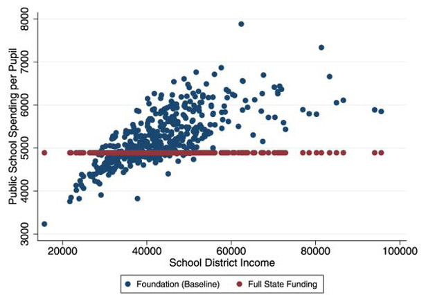
Distribution of public school spending in two educational policies in Ohio.

In this exercise, since the downside hinders intergenerational mobility, rank–rank slope does not fall substantially when we switch to full state funding. Furthermore, implementing an alternative policy to achieve a more equalized distribution of public school spending in a foundation program might be better at improving intergenerational mobility since a foundation program does not place a restriction on public school spending. From this perspective, switching to a full state funding program is not all that favorable.

7. Conclusion

Our paper explores the connection between public school spending and intergenerational mobility in the United States. We argue that the distribution of public school spending across school districts can help account for the variation in rank–rank slope across states. If public school spending is unequally distributed towards rich districts, intergenerational mobility will be low.

We model public school spending through majority voting under two public school finance systems: a full state funding program and a foundation program. Our model extends Fernandez and Rogerson (2003) by taking into account children’s human capital formulation both in school and at work. The highlight of our model is that children’s human capital depends not only on public resources from the state and local government, but also private resources from parents and their own learning ability. We also allow a non-negative parental transfer when children become independent. The estimation results show that our model fits data fairly well. In particular, our model can replicate the positive correlation between the distribution of public school spending and rank–rank slope. However, our estimation was conducted in a limited set of states. This highlights a failure of our model: our simple model is not able to rationalize the behavior in states where the slope coefficient is negative. In this case, a negative value of ρ_h0a would be obtained and rank–rank slope would be negative.

With the estimated model, we conduct three counterfactual simulations to understand the determinants of intergenerational mobility. The first simulation shows that the correlation between parental human capital and a child’s learning ability plays an important role in explaining intergenerational mobility. The second simulation shows that allowing parents to borrow against their children’s future income and using it to invest in their children leads to a more equal distribution of public school spending. The effect on rank–rank slope, however, depends negatively on the correlation between parental human capital and a child’s learning ability. With a smaller correlation, allowing parents to borrow against their children’s future income improves intergenerational mobility significantly. Otherwise, the effect is modest. In the third simulation, we find that switching to a full state funding program also improves intergenerational mobility. Comparing the results of rank–rank slope across simulations in the selected states, however, the impact of switching to a full state funding program is not substantial. This is because imposing statewide taxes only implies that poor school districts are unable to spend much more. Moreover, not allowing local taxes hurts school districts at the middle of the income distribution.

For simplicity, our model abstracts from many interesting features in the real world. For example, we assume there is no heterogeneity in parent income within a school district and children attend public schools in their birth district. If parent income varies within a school district and the parent can choose which school district to reside as in Fernandez and Rogerson (1998), the model may do a better job in capturing rank–rank slopes observed in the data. While endogenizing parental choice of which school district to live in is certainly desirable, we caution here that the few structural models that have been estimated suggest that while differences in amenities across states play an important role, moving costs need to be substantial in order to rationalize the lack of moves in the face of large income differences across states. As more sophisticated data on child income become available (e.g., child income conditional on birthplace), our model can evolve to incorporate migration decisions as well as other features in the real world. We leave these issues for future analysis.

Appendix

Appendix A. State-specific moments not reported in the main text.

State	Moment	Value
Alabama	Average public school spending per pupil in group 1	$4,607
	Average public school spending per pupil in group 2	$4,551
	Average child income in group 1	$19,633
	Average child income in group 2	$20,805
Florida	Average public school spending per pupil in group 2	$5,458
	Average public school spending per pupil in group 3	$5,800
	Average child income in group 2	$19,313
	Average child income in group 3	$21,744
Georgia	Average public school spending per pupil in group 1	$5,106
	Average public school spending per pupil in group 2	$5,101
	Average child income in group 1	$17,324
	Average child income in group 2	$19,318
Illinois	Average public school spending per pupil in group 2	$4,946
	Average public school spending per pupil in group 3	$5,797
	Average child income in group 2	$30,551
	Average child income in group 3	$31,282
Louisiana	Average public school spending per pupil in group 1	$4,666
	Average public school spending per pupil in group 2	$5,282
	Average child income in group 1	$21,475
	Average child income in group 2	$24,166
Maine	Average public school spending per pupil in group 2	$6,337
	Average public school spending per pupil in group 3	$6,367
	Average child income in group 2	$23,934
	Average child income in group 3	$25,172
Maryland	Average public school spending per pupil in group 2	$6,698
	Average public school spending per pupil in group 3	$7,029
	Average child income in group 2	$26,995
	Average child income in group 3	$27,374
Massachusetts	Average public school spending per pupil in group 3	$6,877
	Average public school spending per pupil in group 4	$7,522
	Average child income in group 3	$28,677
	Average child income in group 4	$32,085
Michigan	Average public school spending per pupil in group 2	$6,021
	Average public school spending per pupil in group 3	$6,061
	Average child income in group 2	$25,759
	Average child income in group 3	$28,033
New Hampshire	Average public school spending per pupil in group 2	$6,231
	Average public school spending per pupil in group 3	$6,819
	Average child income in group 2	$27,422
	Average child income in group 3	$28,296
New Jersey	Average public school spending per pupil in group 3	$9,562
	Average public school spending per pupil in group 4	$10,231
	Average child income in group 3	$33,298
	Average child income in group 4	$42,039
Ohio	Average public school spending per pupil in group 2	$5,187
	Average public school spending per pupil in group 3	$6,213
	Average child income in group 2	$26,919
	Average child income in group 3	$26,976
South Carolina	Average public school spending per pupil in group 1	$5,109
	Average public school spending per pupil in group 2	$5,071
	Average child income in group 1	$16,695
	Average child income in group 2	$18,115
Tennessee	Average public school spending per pupil in group 1	$4,623
	Average public school spending per pupil in group 2	$4,716
	Average child income in group 1	$22,202
	Average child income in group 2	$23,043
Virginia	Average public school spending per pupil in group 1	$5,408
	Average public school spending per pupil in group 2	$5,687
	Average child income in group 1	$22,789
	Average child income in group 2	$24,253
West Virginia	Average public school spending per pupil in group 1	$5,611
	Average public school spending per pupil in group 2	$5,483
	Average child income in group 1	$23,908
	Average child income in group 2	$23,962

Appendix B.State-specific estimates not reported in the main text.

Parameter	AL	CO	FL	GA	IL	LA	ME	MD	MA	MI	NH	NJ	OH	SC	TN	VA	WV
μa	0.550	0.756	0.541	0.439	0.734	0.550	0.695	0.695	0.824	0.721	0.724	0.951	0.697	0.570	0.584	0.603	0.544
	(0.004)	(0.014)	(0.004)	(0.006)	(0.004)	(0.004)	(0.002)	(0.012)	(0.012)	(0.002)	(0.004)	(0.008)	(0.004)	(0.002)	(0.004)	(0.028)	(0.002)
σa	0.039	0.103	0.077	0.096	0.454	0.156	0.106	0.107	0.200	0.116	0.271	0.173	0.277	0.048	0.091	0.322	0.031
	(0.002)	(0.036)	(0.026)	(0.002)	(0.010)	(0.008)	(0.004)	(0.020)	(0.002)	(0.002)	(0.004)	(0.010)	(0.094)	(0.006)	(0.014)	(0.032)	(0.004)
ρ h0 a	0.188	0.133	0.060	0.261	0.045	0.250	0.082	0.107	0.407	0.209	0.261	0.198	0.256	0.141	0.147	0.320	0.174
	(0.036)	(0.024)	(0.029)	(0.028)	(0.008)	(0.030)	(0.016)	(0.045)	(0.020)	(0.018)	(0.042)	(0.032)	(0.099)	(0.040)	(0.056)	(0.034)	(0.075)

Note: standard errors in parentheses.

References

- Abbott B, Gallipoli G, 2014. Skill Complementarity and the Geography of Intergenerational Mobility. Working Paper University of British Columbia. [Google Scholar]
- American Education Finance Association, 1992. Public School Finance Programs of the United States and Canada 1990–1991 editions, Blacksburg, VA. [Google Scholar]
- American Education Finance Association, 1995. Public School Finance Programs of the United States and Canada 1993–1994 editions, Blacksburg, VA. [Google Scholar]
- Becker GS, Tomes N, 1979. An equilibrium theory of the distribution of income and intergenerational mobility. Journal of Political Economy 87 (6), 1153–1189. [Google Scholar]
- Becker GS, Tomes N, 1986. Human capital and the rise and fall of families. Journal of Labor Economics 4 (3), S1–S39. [DOI] [PubMed] [Google Scholar]
- Ben-Porath Y, 1967. The production of human capital and the life cycle of earnings. Journal of Political Economy 75, 352–365. [Google Scholar]
- Biasi B, 2015. School Finance Equalization and Intergenerational Income Mobility: Does Equal Spending Lead to Equal Opportunities? Working Paper Stanford University. [Google Scholar]
- Card D, Payne AA, 2002. School finance reform, the distribution of school spending, and the distribution of student test scores. Journal of Public Economics 83 (1), 49–82. [Google Scholar]
- Caucutt EM, Lochner L, 2012. Early and Late Human Capital Investments, Borrowing Constraints, and the Family. Working Paper 18493 NBER. [Google Scholar]
- Chetty R, Hendren N, Kline P, Saez E, 2014. Where is the land of opportunity? The geography of intergenerational mobility in the United States. The Quarterly Journal of Economics 129 (4), 1553–1623. [Google Scholar]
- Corak M, 2013. Income inequality, equality of opportunity, and intergenerational mobility. The Journal of Economic Perspectives 27 (3), 79–102. [Google Scholar]
- Cunha F, Heckman J, 2007. The technology of skill formation. The American Economic Review 97 (2), 31–47. [Google Scholar]
- Epple D, Ferreyra MM, 2008. School finance reform: assessing general equilibrium effects. Journal of Public Economics 92 (5), 1326–1351. [Google Scholar]
- Fernandez R, Rogerson R, 1998. Public education and income distribution: a dynamic quantitative evaluation of education-finance reform. The American Economic Review 88 (4), 813–833. [Google Scholar]
- Fernandez R, Rogerson R, 1999. Education finance reform and investment in human capital: lessons from California. Journal of Public Economics 74 (3), 327–350. [Google Scholar]
- Fernandez R, Rogerson R, 2003. Equity and resources: an analysis of education finance systems. Journal of Political Economy 111 (4), 858–897. [Google Scholar]
- Ferreyra MM, 2009. An empirical framework for large-scale policy analysis, with an application to school finance reform in Michigan. American Economic Journal: Economic Policy 1 (1), 147–180. [Google Scholar]
- Holter HA, 2015. Accounting for cross-country differences in intergenerational earnings persistence: the impact of taxation and public education expenditure. Quantitative Economics 6 (2), 385–428. [Google Scholar]
- Hoxby CM, 2001. All school finance equalizations are not created equal. The Quarterly Journal of Economics 116 (4), 1189–1231. [Google Scholar]
- Jackson CK, Johnson RC, Persico C, 2016. The effects of school spending on educational and economic outcomes: evidence from school finance reforms. The Quarterly Journal of Economics 131 (1), 157–218. [Google Scholar]
- Lee SY, Seshadri A, 2014. On the Intergenerational Transmission of Economic Status. Working Paper University of Wisconsin-Madison. [Google Scholar]
- Lee SYT, Roys N, Seshadri A, 2015. The Causal Effect of Parents’ Education on Children’s Earnings. Working Paper University of Wisconsin–Madison. [Google Scholar]
- Mazumder B, 2005. Fortunate sons: new estimates of intergenerational mobility in the United States using social security earnings data. Review of Economics and Statistics 87 (2), 235–255. [Google Scholar]
- Mincer JA, 1974. Age and experience profiles of earnings. In: Schooling, Experience, and Earnings. NBER, pp. 64–82. [Google Scholar]
- Newey WK, McFadden D, 1994. Large sample estimation and hypothesis testing. In: Handbook of Econometrics, vol. 4, pp. 2111–2245. [Google Scholar]
- Restuccia D, Urrutia C, 2004. Intergenerational persistence of earnings: the role of early and college education. The American Economic Review 94 (5), 1354–1378. [Google Scholar]
- Solon G, 1992. Intergenerational income mobility in the United States. The American Economic Review 82 (3), 393–408. [Google Scholar]