Abstract
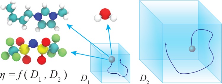
A method is proposed for calculating the shear viscosity of a liquid from finite-size effects of self-diffusion coefficients in Molecular Dynamics simulations. This method uses the difference in the self-diffusivities, computed from at least two system sizes, and an analytic equation to calculate the shear viscosity. To enable the efficient use of this method, a set of guidelines is developed. The most efficient number of system sizes is two and the large system is at least four times the small system. The number of independent simulations for each system size should be assigned in such a way that 50%–70% of the total available computational resources are allocated to the large system. We verified the method for 250 binary and 26 ternary Lennard-Jones systems, pure water, and an ionic liquid ([Bmim][Tf2N]). The computed shear viscosities are in good agreement with viscosities obtained from equilibrium Molecular Dynamics simulations for all liquid systems far from the critical point. Our results indicate that the proposed method is suitable for multicomponent mixtures and highly viscous liquids. This may enable the systematic screening of the viscosities of ionic liquids and deep eutectic solvents.
1. Introduction
The shear viscosity plays an important role in quantifying the required energy for mechanical and chemical processes, and it is essential for solving the Navier–Stokes equations. Various empirical/semiempirical models for predicting the shear viscosity have been developed, including equations of state combined with scaling relations,1−11 free-volume theory,12 friction theory,13 as well as fitting to functional forms.14,15 Alternatively, the shear viscosity can be computed via equilibrium or nonequilibrium molecular dynamics (MD) simulations.7,8,16−24 In nonequilibrium MD (NEMD), the viscosity is calculated from the response of the system to an external shear field.18,25−29 Although NEMD is computationally efficient at large external fields,17,30 the computed viscosity can depend on the applied shear rate.20,21 In equilibrium MD (EMD), the shear viscosity can be computed from the Einstein relation:31−34
| 1 |
where Pαβ represents the off-diagonal components of the stress tensor (i.e., Pxy, Pxz, and Pyz), kB is the Boltzmann constant, t is the correlation time, and V and T are the volume and temperature of the system, respectively. The angle brackets denote an ensemble average. Since the stress tensor is defined for the entire simulation box, the shear viscosity is a property of the system as a whole. This means that an increase in the system size does not improve the statistical uncertainty of the computed shear viscosity.35 Due to the slow relaxation of highly viscous fluids such as ionic liquids14,36 and deep eutectic solvents,37 and due to the large fluctuations in the components of the stress tensor17 (see Figure S1 in the Supporting Information), very long MD simulations are required to sufficiently sample the stress tensor components.
Unlike the shear viscosity, the self-diffusivity is a single-molecule property and can be calculated from the mean-squared displacement (MSD) of all individual molecules of the same species:34,38−40
| 2 |
where rj,i(t) is the position of the jth molecule of species i at time t, and Ni is the number of molecules of species i in the system. The statistical uncertainties of self-diffusivities decrease as the number of molecules in the system increases.35,41,42 The simulation length needed to obtain a linear relation between the MSD and time is much smaller than the length of an MD simulation required for computing the shear viscosity. Therefore, accurate self-diffusivities can be computed from short MD simulations with a large number of molecules. In the same short simulation, such a high accuracy cannot be achieved for the shear viscosity due to the smaller number of samples for the stress tensor components.35
Typical MD simulations for computing transport properties use hundreds to thousands of molecules, which is orders of magnitude smaller than the thermodynamic limit. To overcome this issue, simulation boxes with periodic boundary conditions are used.38 While this approach mimics the presence of an infinite bulk system surrounding the simulated system, computed properties may depend on the size of the simulation box. Large finite-size effects for thermodynamic properties such as activity coefficients,43 chemical potentials,44 and Kirkwood–Buff coefficients45,46 have been reported in literature. In the case of transport properties, self-diffusion coefficients computed from MD simulations depend strongly on the system size while the shear viscosity does not show any system-size dependency.47−49 Dünweg and Kremer50 showed a linear increase of the self-diffusivity of polymers in a good solvent with the inverse of the simulation box length. Yeh and Hummer47 investigated the system-size dependency of computed self-diffusivities of pure liquids, consisting of spherical molecules, and derived a relation between the infinite (Dself∞) and finite-size (Dself) self-diffusivity:47
| 3 |
where DYH is the finite-size correction, here referred to as the Yeh–Hummer (YH) correction, L is the length of the simulation box, which is proportional to N1/3, where N is the number of molecules, η is the shear viscosity of the liquid, and ξ is a dimensionless constant equal to 2.837297 for a cubic simulation box with periodic boundary conditions.47,51−53 For the derivation of this analytic correction, Yeh and Hummer47 used a hydrodynamic model of a spherical particle diffusing in a medium of viscosity η in a box with periodic boundary conditions imposed in every direction. In this model, the hydrodynamic interactions of the particle with the surrounding molecules and the periodic images affect the self-diffusion coefficient. The finite-size effect of the self-diffusivity is caused from the latter, i.e., the self-interaction of the particle through the periodic boundaries. Based on this hydrodynamic model, Yeh and Hummer47 derived eq 3 for spherical particles and verified this correction for a single-component Lennard-Jones (LJ) fluid and pure water. Moultos et al.48 showed that the YH correction is also applicable to molecules of varying size and shape, such as n-alkanes and glymes, provided that the system size exceeds 250 molecules.
In the studies by Spångberg et al.,54 Kühne et al.,55 and others,56−58 the shear viscosities and self-diffusivities of water in the thermodynamic limit were calculated from eq 3. In these studies, several systems sizes were used to compute finite-size self-diffusivities, which were then fitted with a linear regression. To the best of our knowledge, the computation of shear viscosities from finite-size self-diffusivities has not been considered previously for multicomponent mixtures or highly viscous liquids. In this study, we use weighted least-squares linear regression analysis to develop a well-structured methodology for computing shear viscosities from finite-size effects of self-diffusivities. To allocate the available computational resources efficiently, a set of guidelines for choosing simulation parameters, such as the optimum number of system sizes and their size differences is provided. The application of the proposed method is verified for pure water, a large number of binary and ternary LJ systems, and the ionic liquid [Bmim][Tf2N].
This paper is organized in five sections. The proposed method is described in Section 2. In Section 3, details of MD simulations are briefly explained. The results of the MD simulations for pure water, binary and ternary LJ systems, and [Bmim][Tf2N] are discussed in Section 4, along with a set of guidelines for the efficient use of the proposed method. The conclusions are provided in Section 5.
2. Method
To develop a systematic method to compute shear viscosities from the finite-size effects of self-diffusivities, we write eq 3 in a linear form, y = ax + b:
| 4 |
where −ξkBT/6πL and DselfMD are the independent and dependent variables, respectively. The intercept of this line with the vertical axis (L → ∞) is the self-diffusivity in the thermodynamic limit, Dself. The inverse of the slope is the shear viscosity of the fluid, η.
To compute the shear viscosity, this method uses self-diffusivities of at least two system sizes. For each system size, the average self-diffusivity and its variance can be estimated from the mean (D̅) and sample variance (S2) of the self-diffusivities computed from several independent simulations:
| 5 |
| 6 |
where Nsim,j is the number of independent simulations for the jth system size and Dk indicates the self-diffusivity computed from the kth independent simulation for system size j. The parameters of interest (1/η and DselfMD) are then fitted to eq 4 with weighted least-squares linear regression.59 The weighted least-squares linear regression is briefly explained in the Supporting Information. The linear regression analysis requires the standard errors (SEs) of the average self-diffusivities for all system sizes. The inverse of squared SEs are used as the weighting factors for each data point. Since no prior knowledge of these SEs is available, the SE of the self-diffusivity of each system size can be estimated from the sample variance:
| 7 |
According to the work of Pranami and Lamm,41 multiple independent simulations are required to correctly compute the sample variance of the mean self-diffusivity. For a single MD simulation, the computed MSD depends on the initial configuration regardless of the simulation length. Weighted least-squares linear regression analysis yields both the averages and the variances of the parameters in eq 4. The self-diffusivity in the thermodynamic limit is a direct outcome of this analysis. The average shear viscosity is equal to the inverse of the average slope of the fitted line, a̅. If this slope has a statistical uncertainty of δa, the statistical uncertainty of the shear viscosity, δη, can be calculated from error propagation:
| 8 |
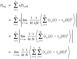
In a recent study, we showed that finite-size corrections to self-diffusivities of different species in a mixture are identical and equal to the YH correction (eq 3).49 This conclusion is based on a detailed study of 250 binary LJ systems with a wide range of LJ energy (ε), size (σ), and mass (m) ratios. The results show that the viscosity of a mixture can be predicted from the finite-size effects of the self-diffusivity of each species regardless of the mass or size ratios. To maximize the statistical information on a single simulation, we introduce a new quantity, the average self-diffusivity (Davg), which is the arithmetic mean of the self-diffusion coefficients of all species, weighted by their corresponding mole fractions. By using the definition of the MSD in multicomponent mixtures (eq 2),60−62 it can be shown that Davg is constructed from the self-diffusion of all molecules in the mixture:
 |
9 |
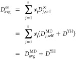
where n and N are the total number of species and molecules in the mixture, respectively, and xi is the mole fraction of species i. Since the self-diffusivities of all species experience an identical finite-size effect,49 the same YH correction (eq 3) can be applied to Davg:
 |
10 |
By combining eqs 4 and 10, the shear viscosity of a mixture can be obtained from Davg, similar to the approach used for pure liquids. Hereafter, the proposed method will be called the D-based method, and ηD-based denotes the corresponding computed shear viscosity.
The D-based method can be used to compute shear viscosities of highly viscous systems such as ionic liquids and deep eutectic solvents. The shear viscosity of these systems can be as large as several hundred cP at room temperature.37,63−65 The length of MD simulations for computing self-diffusivities depends directly on how fast the constituent ions diffuse in the bulk liquid. In MD simulations, Fickian diffusion is observed at time scales in which a linear relation between the MSD and time (i.e., a slope of 1 on a log–log plot) is established.66 However, this criterion does not ensure Gaussian diffusion, which corresponds to a Gaussian distribution for the displacement probability of ions.67 Ionic liquids and deep eutectic solvents consist of highly associated pairs of ions and temporarily form cages.68 While cage effects can also be present in simple fluids,69 it plays an important role in determining the minimum length of an MD simulation for ionic systems.68,70 As discussed in detail in the work of Casalegno et al.,68 for short time scales, each ion fluctuates around a certain position in the cage. Due to dynamical heterogeneity,67,68,71 a non-Gaussian distribution is observed for the diffusion probability of ions trapped in the cage. For longer time scales, ions jump from a cage to another. The displacement probability forms a Gaussian distribution corresponding to Gaussian diffusion.68 According to Casalegno et al.,68 for room-temperature ionic liquids, a rough estimate of the time scale corresponding to Gaussian diffusion can be made based on a minimum average displacement of 1.5 nm for all constituent ions. This criterion ensures that the simulation time is sufficiently long for all ions to break the local ion cages and diffuse in the bulk liquid.70,72 This criterion can be used for room-temperature ionic liquids for performing long enough MD simulations to compute finite-size self-diffusivities with the D-based method.
3. Simulation Details
To validate the D-based method, three different systems are considered: binary and ternary LJ systems, pure water, and the ionic liquid [Bmim][Tf2N]. All MD simulations are carried out with LAMMPS (version 16, Feb 2016).73 The order-n algorithm is used for an efficient sampling of time correlations for the calculation of self-diffusivities and shear viscosities.66
MD simulations of 26 ternary LJ systems were carried out. The results for 250 binary LJ systems are obtained from the Supporting Information of our previous work, ref (49). For the interaction between dissimilar LJ particles (i and j), we use the Lorentz–Berthelot mixing rules with a modification factor (kij) to include nonideality in the systems:34
 |
11 |
where ε and σ are the parameters of the LJ potential. The simulation parameters of all binary and ternary systems are provided in Tables 1 and 2, respectively. All parameters are reported in reduced units, where σ1 = σ = 1, ε1 = ε = 1, and m1 = m = 1 (mass) are the basis units.34 All LJ interactions are truncated and shifted at a cutoff radius of 4σ. Simulations for two system sizes (500 and 4000 LJ particles) were performed at a reduced temperature of 0.65 and a reduced pressure of 0.05. The number densities of the binary49 and ternary systems are in the range of 0.14–0.89 and 0.78–0.88, respectively. An integral time step of 0.001 is used, and the simulation lengths of the binary and ternary systems are 200 million and 100 million time steps, respectively.
Table 1. Specifications of 250 Binary LJ Systems at a Temperature of 0.65 and a Pressure of 0.0549a.
| specification | values |
|---|---|
| x1 | 0.1, 0.3, 0.5, 0.7, 0.9 |
| ε2/ε1 | 1.0, 0.8, 0.6, 0.5 |
| σ2/σ1 | 1.0, 1.2, 1.4, 1.6 |
| m2/m1 | (σ2/σ1)3 |
| kij | 0.05, 0.0, −0.3, −0.6 |
Table 2. Specifications of 26 Ternary LJ Systems at a Temperature of 0.65 and a Pressure of 0.05a.
| specification | values |
|---|---|
| k12 | 0.05, −0.3, −0.6 |
| k13 | 0.05, −0.3, −0.6 |
| k23 | 0.05, 0.0, −0.3, −0.6 |
The LJ interaction parameters of species 1, 2, and 3 are ε1 = ε = 1.0, ε2 = 0.8, and ε3 = 0.6, respectively. All species have the same size (σ1 = σ2 = σ3 = σ = 1.0) and mass (m1 = m2 = m3 = 1.0). All values are reported in reduced units.34xi indicates the mole fraction of species i, where x1 = 0.4, x2 = 0.3, and x3 = 0.3.
For the molecular systems, the initial configurations were made in Packmol,74 and the LAMMPS input files were created with VMD.75 The three-site SPC/E model is used for water.76 The force field parameters of [Bmim][Tf2N] are obtained from the work of Zhang et al.77 The LJ interactions for water and the ionic liquid are truncated at 9 and 12 Å, respectively, with analytic tail corrections considered for energy and pressure. The particle–particle particle–mesh (PPPM) method with a relative precision of 10–6 is used for the long-range electrostatic interactions. The Verlet algorithm is used to integrate Newton’s equations of motion with a time step of 1 fs. MD simulations for water performed at 298 K and 1 atm. MD simulations of [Bmim][Tf2N] were performed at three temperatures of 300, 400, and 500 K and a pressure of 1 atm. The simulation times used for computing shear viscosities of water and [Bmim][Tf2N] are 50 and 200 ns, respectively. Self-diffusivities of water and [Bmim][Tf2N] are computed from independent simulations of 0.5 and 20 ns, respectively. Due to the slow relaxation of [Bmim][Tf2N] at 300 K, MD simulations of 50 and 450 ns are needed to obtain the self-diffusivities and shear viscosity at this low temperature, respectively. The choice of these simulation lengths is made so that a minimum average displacement of 1.5 nm is obtained for all systems (discussed thoroughly in Section 2).
4. Results and Discussions
Pure Water
A set of simulations consisting of seven system sizes—250, 500, 1000, 2000, 4000, 8000, and 16 000 water molecules—was carried out. The average self-diffusivities were obtained from 100 independent simulations of 0.5 ns for each system size. In Figure 1, the average self-diffusivities of water are shown as a function of the system size. These finite-size self-diffusivities lie on the line fitted to eq 4:
| 12 |
where N equals the number of water molecules in the simulation box. From the intercept with the vertical axis, the self-diffusivity of the SPC/E water model in the thermodynamic limit at 298 K and 1 atm is estimated to be (2.870 ± 0.004) × 10–9 m2 s–1 and the shear viscosity 0.708 ± 0.014 cP. The shear viscosity of water computed from the Einstein relation (eq 1) is 0.694 ± 0.010 cP. These two values are in excellent agreement, considering the wide range of shear viscosities reported in the literature for the SPC/E water model at the same conditions: 0.68,56 0.71,54 0.729,78,79 and 0.82 cP.80 This agreement confirms the applicability of the D-based method for pure water.
Figure 1.
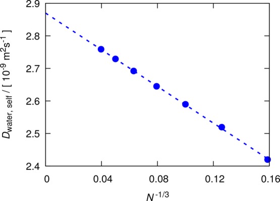
Computed self-diffusion coefficients of the SPC/E water model at 298 K and 1 atm for seven system sizes: N = 250, 500, 1000, 2000, 4000, 8000, and 16 000 water molecules. A total of 100 independent simulations of 0.5 ns were performed for each system size. The dashed line is fitted with the weighted least-squares linear regression (eq 12) to the YH equation (eq 4). Error bars are smaller than the symbol sizes. The self-diffusivities are tabulated in Table S1 of the Supporting Information.
The extensive data set of finite-size water self-diffusivities provides a suitable estimation of the variances (S2) and the standard deviations (S) of self-diffusivities as a function of the system size. These standard deviations will be used in the next section for optimizing the D-based method. Figure 2 shows the estimated standard deviations as a function of the number of molecules (N–1/3). Since no prior knowledge of the functional form is available, an initial guess for the functional form would be a power-law function (aNb) with two fitting parameters:
| 13 |
The exponent −0.31 and the linear arrangement of the data points in Figure 2 suggest that the standard deviation can also be a linear function in N–1/3, which decreases the number of fitting parameters to one (aN–1/3):
| 14 |
Figure 2.
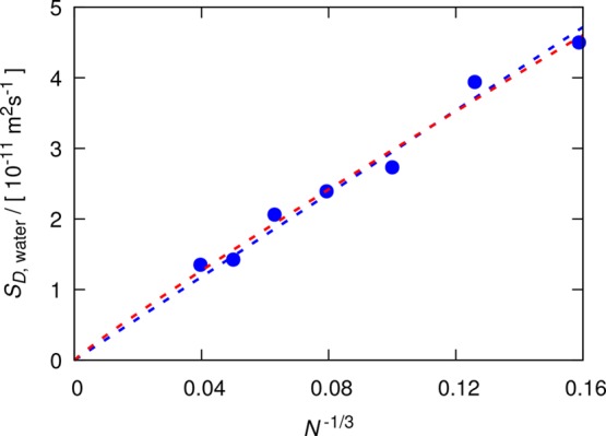
Estimated standard deviations of the self-diffusion coefficients of the SPC/E water model at 298 K and 1 atm, computed for seven system sizes: N = 250, 500, 1000, 2000, 4000, 8000, and 16 000 water molecules. A total of 100 independent simulations of 0.5 ns were performed for each system size. The red and blue dashed lines are fits to a power-law (eq 13) and a linear function (eq 14), respectively.
In the next section, eq 14 combined with eq 12 will be used as a model for the normal distribution of finite-size self-diffusivities of water as a function of system size.
Optimization
In this section, a set of optimum simulation parameters for which the computed shear viscosities have a minimum statistical uncertainty is proposed. The following parameters are considered: the number of system sizes, the size difference between systems, and the allocation of computational resources to each system size. The size difference between system i and system j is normalized by the size of the smallest system (system 1): (Nj – Ni)/N1. According to the work of Moultos et al.,48 the smallest system should contain at least 250 molecules. This criterion ensures that the YH correction (eq 3) provides an accurate prediction for the finite-size effects of self-diffusivities. As a constraint on the optimization problem, the total computational resources are fixed. The computational resources scale linearly with the number of independent simulations (Nsim,i) and polynomially with the number of molecules (Ni) in the simulation box, depending on computer hardware, the employed computational methods, and the scalability of MD simulations.34 Thus, the ratio, α, between the computational resources allocated to system i and system j is
| 15 |
where γ indicates the scalability of MD simulations. Two values of γ are considered here for the scalability of MD simulations: γ = 1 and 2. For γ = 1, computational requirements grow linearly with the system size. For γ = 2, the growth in computational requirements is quadratic and thus faster than the linear growth. Current state-of-the-art MD packages73,81,82 have a good computational scalability, γ, close to 1.
The simulation results presented for the SPC/E water model can be used as a basis for finding the optimum combination of the simulation parameters for the D-based method. eqs 4 and 14 are used to model the average and standard deviation of finite-size self-diffusivity of water as a function of system size. This model enables us to predict the self-diffusivity of water for a hypothetical MD simulation with a specified number of molecules. This can be achieved by generating a random number from a normal distribution with a mean self-diffusivity and a standard deviation determined by eqs 12 and 14. For a set of simulations with a number of system sizes and independent simulations per system size, a set of finite-size self-diffusivities is constructed and the corresponding shear viscosity is calculated from the D-based method. Since this shear viscosity depends on the set of finite-size self-diffusivities, the procedure should be repeated for many times and all shear viscosities are recorded in a histogram. For a specific set of simulation parameters, the data stored in the histogram yield an estimate for the variance (S2) and standard deviation (S) of the shear viscosity. The aim of this optimization procedure is to find the simulation parameters that minimize the standard deviation (S) of the shear viscosity.
The first scenario considered here is the optimization for two system sizes. The simulation parameters studied are (i) the normalized size difference ((N2 – N1)/N1), and (ii) the ratio between the computational resources allocated to system 1 and 2 (α). The objective function is the estimated standard deviation of shear viscosities normalized by Smin, the global minimum estimated standard deviation of the shear viscosity for a specified value of γ and all values of α and (N2 – N1)/N1. In Figure 3, the normalized estimated standard deviations (S/Smin) are shown for several values of α, ranging from 0.2 to 5.0, and the two values of γ. As can be seen in Figure 3, a range of α between 1 and 2 yields the smallest value of S/Smin. This means that the number of independent simulations for each system size should be distributed in such a way that 50%–70% of the computational resources is allocated to the large system. Furthermore, it can be observed that the large system should be at least 4 times the size of the small system. Depending on the scalability of MD simulations, the optimum normalized size difference ((N2 – N1)/N1) ranges from 3 (γ = 2) to 40 (γ = 1).
Figure 3.
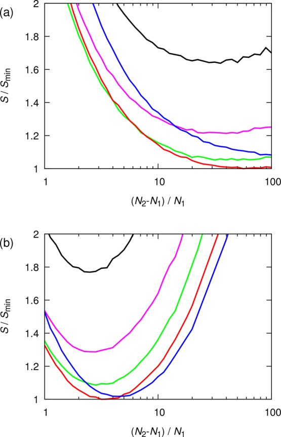
Normalized estimated standard deviation (S/Smin) of the shear viscosity as a function of the normalized size difference between two systems ((N2 – N1)/N1). The total amount of computational resources is fixed. Different colors indicate various ratios α of the computational resources allocated to large and small system sizes (eq 15): 0.2 (black), 0.5 (magenta), 1.0 (green), 2.0 (red), and 5.0 (blue). Two types of scalability for MD simulations are considered: (a) high scalability (γ = 1) and (b) low scalability (γ = 2).
A similar investigation can be carried out for three system sizes. Here, α is set to 1, indicating that the computational resources are equally distributed between the three system sizes. In Figure 4, normalized estimated standard deviations (S/Smin) are shown as a function of the normalized size difference between the small and medium systems ((N2 – N1)/N1), and the medium and large systems ((N3 – N2)/N1). Figure 4a (γ = 1) shows that a minimum cost function (S/Smin) is achieved for (N2 – N1)/N1 > 10. This suggests that, while the choice of the size difference between the small and medium systems is important, the size difference between the medium and large systems does not play a significant role. For very small values of the normalized size difference between the medium and large systems ((N3 – N2)/N1 → 0), it can be deduced that the optimization problem reduces to a problem of two system sizes, which has already been discussed. In Figure 4b, this is also observed for γ = 2. The optimum condition is achieved at (N2 – N1)/N1 = 3, which is in agreement with what is shown in Figure 3b for two system sizes. This suggests that the optimum condition observed for three system sizes can also be achieved with two systems.
Figure 4.
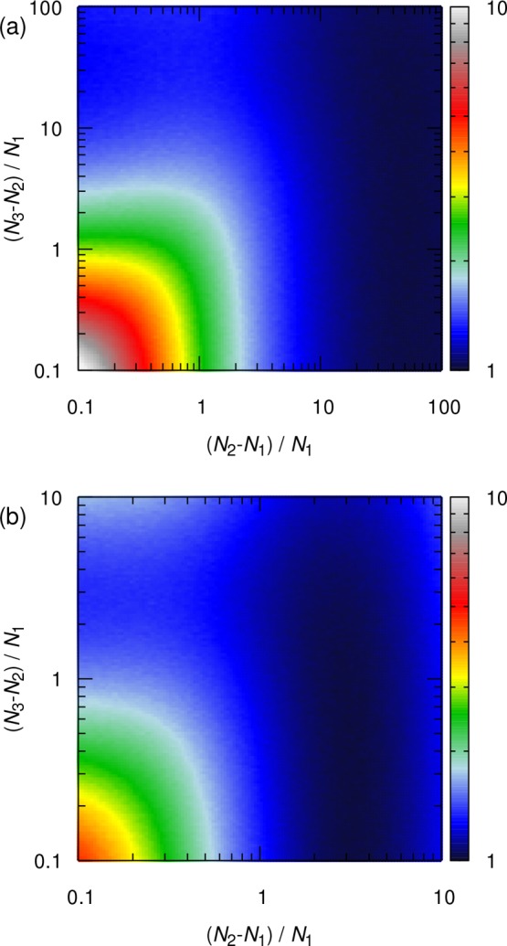
Normalized estimated standard deviations (S/Smin) of the shear viscosities as a function of the normalized size difference between small and medium systems ((N2 – N1)/N1), and between medium and large system sizes ((N3 – N2)/N1). A fixed amount of computational resources is equally distributed between the three system sizes. Two types of scalability for the MD simulations are considered: (a) high scalability (γ = 1) and (b) low scalability (γ = 2).
Based on the optimization results, the use of either two or three system sizes yields optimum shear viscosities. In the case of a limited amount of computational resources, adding more system sizes leads to a smaller number of independent simulations per system size. As a consequence, the limited number of independent simulations leads to poor sampling that may not yield an accurate average and standard deviation for self-diffusivities. This adversely affects the accuracy of average finite-size self-diffusivities and consequently the computed shear viscosity. Hence, the use of more than two system sizes is not justified. The choice of the optimum conditions may vary depending on the MD software73,81,82 as well as the algorithms used in the software (e.g., handling of long-range electrostatic interactions, details of the neighbor lists34). These specifications determine the optimum size of the system and number of independent simulations according to the results shown in Figure 3, and consequently affect the computational requirements of the D-based method.
Lennard-Jones Systems
To examine the accuracy of the D-based method for multicomponent fluid mixtures, the shear viscosities of 250 binary49 and 26 ternary LJ systems were computed. The comparison between the D-based shear viscosities and those computed from the Einstein relation (ηEMD, eq 1) are shown in Figure 5. By varying the characteristics of the studied LJ systems as mentioned in Tables 1 and 2, a wide range of shear viscosities is covered. While all data points show a good agreement between the two methods, the smallest deviation from the diagonal dashed lines is observed for the quantity Davg, for both binary and ternary systems. This is expected since Davg is constructed from the self-diffusivities of all species present in the mixture. Therefore, for multicomponent mixtures, Davg should be used for calculating the shear viscosity rather than the self-diffusivity of only a single species.
Figure 5.
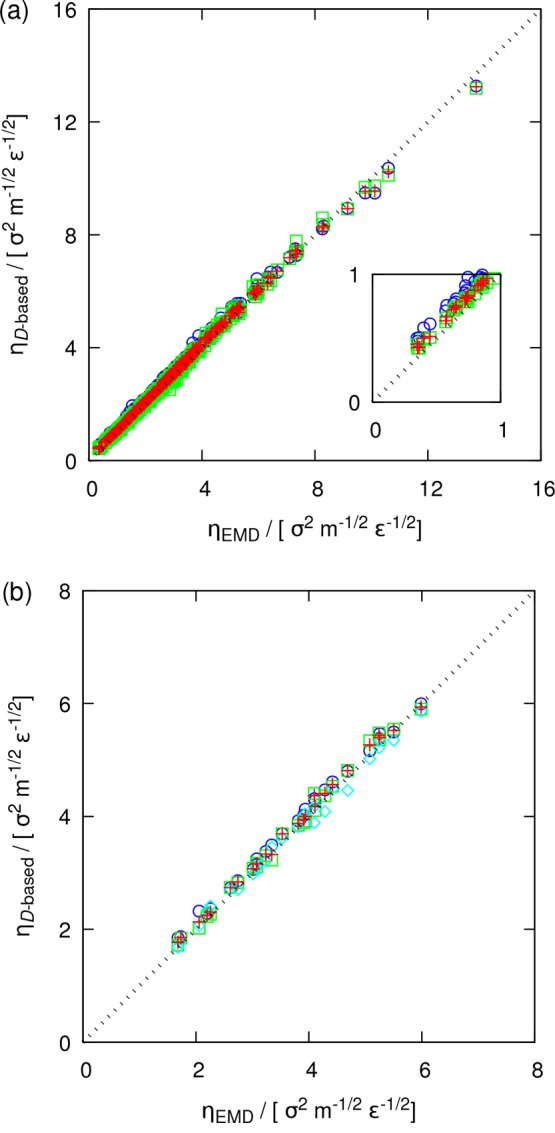
Comparison between the shear viscosities of (a) 250 binary and (b) 26 ternary LJ systems computed from the Einstein relation (ηEMD, eq 1) and the D-based method (ηD-based, eq 4) at a reduced temperature of 0.65 and a reduced pressure of 0.05. The D-based shear viscosities are computed from the self-diffusion coefficients of species 1 (blue circles), species 2 (green squares), and species 3 (cyan diamonds; only for ternary systems) as well as the average self-diffusivity (eq 9, red crosses). Error bars are omitted for clarity. All computed shear viscosities and their statistical uncertainties are listed in the Supporting Information, Tables S4 and S7.
In Figure 5, the maximum deviation from the diagonal line, which represent perfect agreement between the D-based method and the Einstein relation, are observed for binary LJ systems with very low densities (inset of Figure 5a). As discussed in our previous study,49 these outliers have very dissimilar size (σ2/σ1 = 1.4 or 1.6) and interaction (ε2/ε1 = 0.5 or 0.6) parameters. According to the work of Heyes et al.83 for a hard-sphere fluid, the exponent −1/3 in N–1/3 (i.e., L–1) in eq 3 is valid only for a range of packing fractions. Since the validity of the YH correction have been shown for many real molecular liquids,47−50 it is expected that the range of packing fractions for which the YH correction holds correspond to a liquid phase. From Figure 6, a similar observation to the work of Heyes et al.83 can be made for LJ systems. In this figure, the normalized difference between the shear viscosities computed from the D-based method (using Davg) and the Einstein relation is shown as a function of (a) the shear viscosity and (b) the density for all binary and ternary LJ systems. For LJ systems at high densities, a good agreement between the two methods is observed. For the systems with low densities/viscosities, shown also in the inset of Figure 5, substantial deviations (up to 30%) between the D-based method and the Einstein relation are observed. Figure 6 shows that as the density of a system decreases and thus hydrodynamic interactions become weaker, the scaling proposed by Yeh and Hummer does not hold anymore. At low densities, the finite-size effects of self-diffusivities do not scale as N–1/3, and the exponent varies according to the packing fraction of the fluid (e.g., see the work of Heyes et al.83). As discussed briefly in the Supporting Information, the outliers shown in Figures 5 and 6 correspond to conditions close to the critical point. This suggests that neither the YH correction nor the D-based method is applicable at conditions close to the critical point. Nevertheless, our findings show that the D-based method is able to predict accurate shear viscosities for all real molecular systems in a liquid phase far from the critical point.
Figure 6.
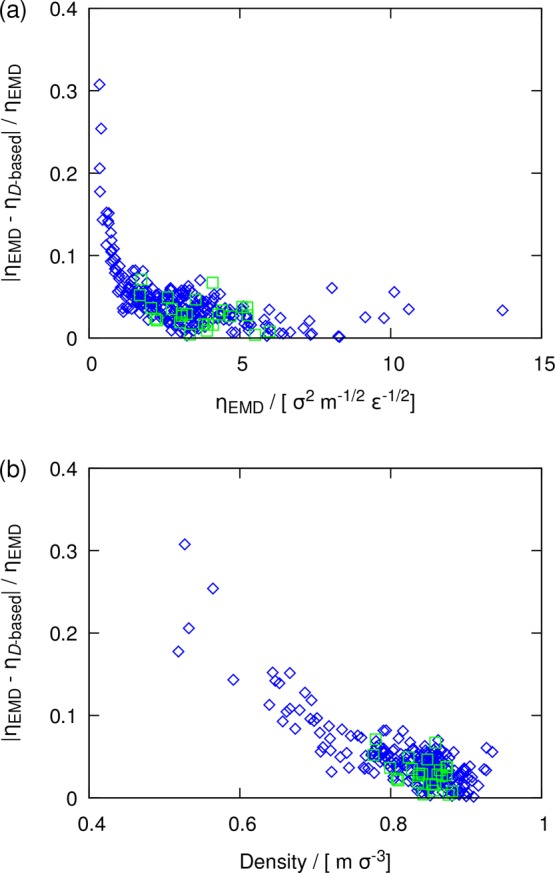
Normalized absolute difference between shear viscosities computed from the Einstein relation and the D-based method as a function of (a) the shear viscosity and (b) the density. Data are shown for binary (blue diamonds) and ternary (green squares) LJ systems at a temperature of 0.65 and a pressure of 0.05. The D-based method shear viscosities are computed from average self-diffusivities (Davg).
[Bmim][Tf2N]
As a representative test case, shear viscosities of the ionic liquid [Bmim][Tf2N] are calculated from the D-based method and the Einstein relation (eq 1) at a pressure of 1 atm and three temperatures: 300, 400, and 500 K. MD simulations of 20 ns were performed for computing self-diffusivities of [Bmim][Tf2N] at 400 and 500 K. To fulfill the minimum average displacement criterion of 1.5 nm (explained in Section 2), the MD simulations at 300 K were carried out for 50 ns. According to the set of guidelines proposed for the D-based method, 40 and 8 independent MD simulations were performed for two systems of 150 and 1200 pairs of ions, respectively.
In Figure 7, the computed self-diffusivities for both [Bmim] and [Tf2N] ions as well as Davg are shown. It can be seen that the finite-size self-diffusivities of [Bmim] and [Tf2N] greatly differ from each other, but the finite-size effects remain equal for both ions and Davg. Therefore, shear viscosities computed from the slopes of the lines connecting finite-size self-diffusivities are equal within the error bars. The computed shear viscosities from the D-based method and the Einstein relation, and their 95% confidence intervals are reported in Table S11 in the Supporting Information. Figure 7 shows that the use of Davg for the D-based method is not limited to molecular mixtures and that this quantity can be used for ionic systems as well.
Figure 7.
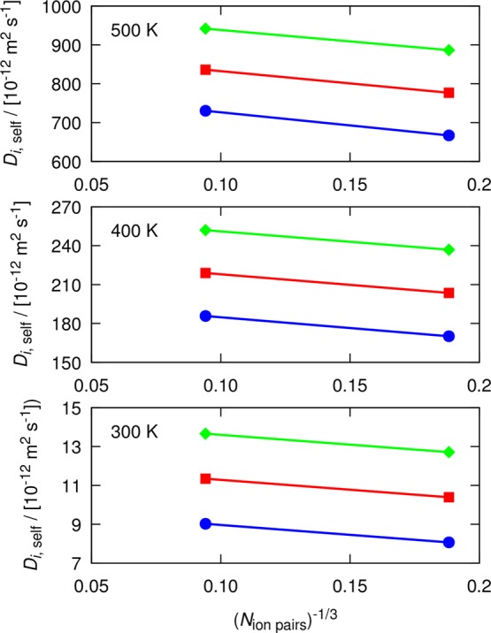
Computed self-diffusion coefficients of [Bmim][Tf2N] at 300, 400, and 500 K and 1 atm. In all, 40 and 8 independent simulations were performed for two system sizes of 150 and 1200 ion pairs, respectively. Self-diffusivities are shown for [Bmim] (blue circles), [Tf2N] (green diamonds), and Davg (red squares). The slope of the line connecting each two points yields the shear viscosity. The simulation length at 400 and 500 K is 20 ns. Simulations at 300 K were performed for 50 ns. All self-diffusivities are listed in Tables S8–S10 of the Supporting Information. Error bars are smaller than the symbol sizes.
Figure 8 shows the computed shear viscosities of the ionic liquid as a function of temperature. The lines are the fits to the Vogel equation:84
| 16 |
where A, B, and C are the coefficients of this equation. For all temperatures, a good agreement is observed between the D-based method, the Einstein relation (eq 1), and the estimates of shear viscosities from the work of Zhang et al.77 This agreement confirms the applicability of the D-based method to complex and highly viscous mixtures of nonspherical molecules/ions. To compute the shear viscosity of any ionic liquid or deep eutectic solvent, the set of guidelines for the D-based method along with the criterion on the minimum average displacement can be used to specify an optimum set of MD simulations.
Figure 8.
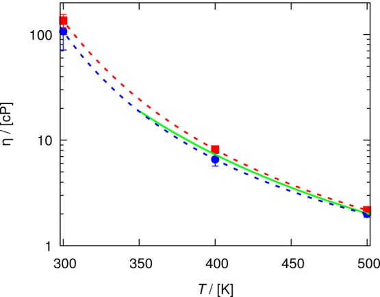
Shear viscosity of [Bmim][Tf2N] as a function of temperature at 1 atm, computed from the D-based method (blue circles, eq 4) and the Einstein relation (red squares, eq 1). The lines are fits to the Vogel equation84 (eq 16) for the D-based method (blue dashed, eq 4), Einstein relation (red dashed), and Green–Kubo relation (green solid; data extracted from the work of Zhang et al.77). The shear viscosities and coefficients of the Vogel equation are provided in Tables S11 and S12 of the Supporting Information.
5. Conclusion
A systematic methodology, called the D-based method, is proposed for accurately computing the shear viscosity of a liquid from the finite-size effects of self-diffusivities. The computational requirements of this method and the statistical uncertainty of the computed viscosity are comparable to the conventional methods, e.g., the Einstein relation. By performing weighted least-squares linear regression analysis, the shear viscosity can be computed from the slope of a line fitted to computed finite-size self-diffusivities. To obtain accurate shear viscosities at a minimum computational requirement, a set of guidelines for this method was proposed. The optimum number of system sizes is two, and depending on the available computational resources and the scalability of the MD simulations, the large system size should be 4–40 times the small system size. The number of independent simulations per system size should be assigned in such a way that 50%–70% of the computational resources is allocated to the MD simulations of the large system. For multicomponent mixtures, the D-based method performs best when the average self-diffusivity of all species (Davg) is used instead of using the self-diffusivity of a single species. The D-based method was verified for pure water, a large number of binary and ternary Lennard-Jones systems, and an ionic liquid ([Bmim][Tf2N]). The results of the D-based method were in good agreement with those obtained from the Green–Kubo and Einstein relations for all molecular systems. These results suggest that the D-based method can be a potential method for computing shear viscosities of highly viscous liquids and multicomponent mixtures.
Acknowledgments
We thank Yong Zhang and Edward Maginn for providing the force field parameters of the ionic liquid [Bmim][Tf2N].77 This work was sponsored by NWO Exacte Wetenschappen (Physical Sciences) for the use of supercomputer facilities, with financial support from the Nederlandse Organisatie voor Wetenschappelijk Onderzoek (Netherlands Organisation for Scientific Research, NWO). T.J.H.V. acknowledges NWO-CW (Chemical Sciences) for a VICI grant.
Supporting Information Available
The Supporting Information is available free of charge on the ACS Publications website at DOI: 10.1021/acs.jctc.8b00625.
Brief overview of weighted least-squares linear regression, computed self-diffusion coefficients and shear viscosities of water, binary and ternary Lennard-Jones systems, and the ionic liquid [Bmim][Tf2N]; critical properties of binary LJ systems; and a short discussion on the fluctuation of the instantaneous pressure in molecular dynamics simulations of liquid water (PDF)
The authors declare no competing financial interest.
Supplementary Material
References
- Teja A. S.; Rice P. Generalized Corresponding States Method for the Viscosities of Liquid Mixtures. Ind. Eng. Chem. Fundam. 1981, 20, 77–81. 10.1021/i100001a015. [DOI] [Google Scholar]
- Ely J. F.; Hanley H. J. M. Prediction of Transport Properties. 1. Viscosity of Fluids and Mixtures. Ind. Eng. Chem. Fundam. 1981, 20, 323–332. 10.1021/i100004a004. [DOI] [Google Scholar]
- Pedersen K. S.; Fredenslund A. An Improved Corresponding States Model for the Prediction of Oil and Gas Viscosities and Thermal Conductivities. Chem. Eng. Sci. 1987, 42, 182–186. 10.1016/0009-2509(87)80225-7. [DOI] [Google Scholar]
- Assael M. J.; Dymond J. H.; Papadaki M.; Patterson P. M. Correlation and Prediction of Dense Fluid Transport Coefficients. I. n-alkanes. Int. J. Thermophys. 1992, 13, 269–281. 10.1007/BF00504436. [DOI] [Google Scholar]
- Rosenfeld Y. Relation between the Transport Coefficients and the Internal Entropy of Simple Systems. Phys. Rev. A: At., Mol., Opt. Phys. 1977, 15, 2545–2549. 10.1103/PhysRevA.15.2545. [DOI] [Google Scholar]
- Rosenfeld Y. A Quasi-Universal Scaling Law for Atomic Transport in Simple Fluids. J. Phys.: Condens. Matter 1999, 11, 5415–5427. 10.1088/0953-8984/11/28/303. [DOI] [Google Scholar]
- Galliéro G.; Boned C.; Baylaucq A. Molecular Dynamics Study of the Lennard-Jones Fluid Viscosity: Application to Real Fluids. Ind. Eng. Chem. Res. 2005, 44, 6963–6972. 10.1021/ie050154t. [DOI] [Google Scholar]
- Galliéro G.; Boned C.; Baylaucq A.; Montel F. Influence of the Mass Ratio on Viscosity in Lennard-Jones Mixtures: The One-fluid Model Revisited Using Nonequilibrium Molecular Dynamics. Fluid Phase Equilib. 2005, 234, 56–63. 10.1016/j.fluid.2005.05.016. [DOI] [Google Scholar]
- Galliero G.; Boned C.; Fernández J. Scaling of the Viscosity of the Lennard-Jones Chain Fluid Model, Argon, and Some Normal Alkanes. J. Chem. Phys. 2011, 134, 064505. 10.1063/1.3553262. [DOI] [PubMed] [Google Scholar]
- Lötgering-Lin O.; Schöniger A.; Nowak W.; Gross J. Bayesian Model Selection Helps To Choose Objectively between Thermodynamic Models: A Demonstration of Selecting a Viscosity Model Based on Entropy Scaling. Ind. Eng. Chem. Res. 2016, 55, 10191–10207. 10.1021/acs.iecr.6b02671. [DOI] [Google Scholar]
- Harris K. R. Scaling the Transport Properties of Molecular and Ionic Liquids. J. Mol. Liq. 2016, 222, 520–534. 10.1016/j.molliq.2016.07.029. [DOI] [Google Scholar]
- Llovell F.; Marcos R. M.; Vega L. F. Free-Volume Theory Coupled with Soft-SAFT for Viscosity Calculations: Comparison with Molecular Simulation and Experimental Data. J. Phys. Chem. B 2013, 117, 8159–8171. 10.1021/jp401307t. [DOI] [PubMed] [Google Scholar]
- Quiñones-Cisneros S. E.; Zéberg-Mikkelsen C. K.; Fernández J.; García J. General Friction Theory Viscosity Model for the PC-SAFT Equation of State. AIChE J. 2006, 52, 1600–1610. 10.1002/aic.10755. [DOI] [Google Scholar]
- Wang X.; Chi Y.; Mu T. A Review on the Transport Properties of Ionic Liquids. J. Mol. Liq. 2014, 193, 262–266. 10.1016/j.molliq.2014.03.011. [DOI] [Google Scholar]
- Alcalde R.; García G.; Atilhan M.; Aparicio S. Systematic Study on the Viscosity of Ionic Liquids: Measurement and Prediction. Ind. Eng. Chem. Res. 2015, 54, 10918–10924. 10.1021/acs.iecr.5b02713. [DOI] [Google Scholar]
- Mondello M.; Grest G. S. Viscosity Calculations of n-Alkanes by Equilibrium Molecular Dynamics. J. Chem. Phys. 1997, 106, 9327. 10.1063/1.474002. [DOI] [Google Scholar]
- Hess B. Determining the Shear Viscosity of Model Liquids from Molecular Dynamics Simulations. J. Chem. Phys. 2002, 116, 209. 10.1063/1.1421362. [DOI] [Google Scholar]
- Borodin O.; Smith G. D.; Kim H. Viscosity of a Room Temperature Ionic Liquid: Predictions from Nonequilibrium and Equilibrium Molecular Dynamics Simulations. J. Phys. Chem. B 2009, 113, 4771–4774. 10.1021/jp810016e. [DOI] [PubMed] [Google Scholar]
- Chen T.; Smit B.; Bell A. T. Are Pressure Fluctuation-based Equilibrium Methods Really Worse than Nonequilibrium Methods for Calculating Viscosities?. J. Chem. Phys. 2009, 131, 246101. 10.1063/1.3274802. [DOI] [PubMed] [Google Scholar]
- Tenney C. M.; Maginn E. J. Limitations and Recommendations for the Calculation of Shear Viscosity using Reverse Nonequilibrium Molecular Dynamics. J. Chem. Phys. 2010, 132, 014103. 10.1063/1.3276454. [DOI] [PubMed] [Google Scholar]
- Van-Oanh N.-T.; Houriez C.; Rousseau B. Viscosity of the 1-ethyl-3-methylimidazolium Bis(trifluoromethylsulfonyl)imide Ionic Liquid from Equilibrium and Nonequilibrium Molecular Dynamics. Phys. Chem. Chem. Phys. 2010, 12, 930–936. 10.1039/B918191A. [DOI] [PubMed] [Google Scholar]
- Orozco G. A.; Moultos O. A.; Jiang H.; Economou I. G.; Panagiotopoulos A. Z. Molecular Simulation of Thermodynamic and Transport Properties for the H2O+NaCl System. J. Chem. Phys. 2014, 141, 234507. 10.1063/1.4903928. [DOI] [PubMed] [Google Scholar]
- Jiang H.; Mester Z.; Moultos O. A.; Economou I. G.; Panagiotopoulos A. Z. Thermodynamic and Transport Properties of H2O + NaCl from Polarizable Force Fields. J. Chem. Theory Comput. 2015, 11, 3802–3810. 10.1021/acs.jctc.5b00421. [DOI] [PubMed] [Google Scholar]
- Moultos O. A.; Tsimpanogiannis I. N.; Panagiotopoulos A. Z.; Trusler J. P. M.; Economou I. G. Atomistic Molecular Dynamics Simulations of Carbon Dioxide Diffusivity in n-Hexane, n-Decane, n-Hexadecane, Cyclohexane, and Squalane. J. Phys. Chem. B 2016, 120, 12890–12900. 10.1021/acs.jpcb.6b04651. [DOI] [PubMed] [Google Scholar]
- Müller-Plathe F. Reversing the Perturbation in Nonequilibrium Molecular Dynamics: An Easy Way to Calculate the Shear Viscosity of Fluids. Phys. Rev. E: Stat. Phys., Plasmas, Fluids, Relat. Interdiscip. Top. 1999, 59, 4894–4898. 10.1103/PhysRevE.59.4894. [DOI] [PubMed] [Google Scholar]
- Bordat P.; Müller-Plathe F. The Shear Viscosity of Molecular Fluids: A Calculation by Reverse Nonequilibrium Molecular Dynamics. J. Chem. Phys. 2002, 116, 3362–3369. 10.1063/1.1436124. [DOI] [Google Scholar]
- Kelkar M. S.; Maginn E. J. Rapid shear viscosity calculation by momentum impulse relaxation molecular dynamics. J. Chem. Phys. 2005, 123, 224904. 10.1063/1.2131060. [DOI] [PubMed] [Google Scholar]
- Kelkar M. S.; Maginn E. J. Effect of Temperature and Water Content on the Shear Viscosity of the Ionic Liquid 1-Ethyl-3-methylimidazolium Bis(trifluoromethanesulfonyl)imide As Studied by Atomistic Simulations. J. Phys. Chem. B 2007, 111, 4867–4876. 10.1021/jp0686893. [DOI] [PubMed] [Google Scholar]
- Hartkamp R.; Bernardi S.; Todd B. D. Transient-Time Correlation Function Applied to Mixed Shear and Elongational Flows. J. Chem. Phys. 2012, 136, 064105. 10.1063/1.3684753. [DOI] [PubMed] [Google Scholar]
- Arya G.; Maginn E. J.; Chang H.-C. Efficient Viscosity Estimation from Molecular Dynamics Simulation via Momentum Impulse Relaxation. J. Chem. Phys. 2000, 113, 2079. 10.1063/1.482019. [DOI] [Google Scholar]
- Zwanzig R. Time-Correlation Functions and Transport Coefficients in Statistical Mechanics. Annu. Rev. Phys. Chem. 1965, 16, 67–102. 10.1146/annurev.pc.16.100165.000435. [DOI] [Google Scholar]
- Schoen M.; Hoheisel C. The Shear Viscosity of a Lennard-Jones Fluid Calculated by Equilibrium Molecular Dynamics. Mol. Phys. 1985, 56, 653–672. 10.1080/00268978500102591. [DOI] [Google Scholar]
- Meier K.; Laesecke A.; Kabelac S. Transport coefficients of the Lennard-Jones model fluid. I. Viscosity. J. Chem. Phys. 2004, 121, 3671–3687. 10.1063/1.1770695. [DOI] [PubMed] [Google Scholar]
- Allen M. P.; Tildesley D. J.. Computer Simulation of Liquids, 2nd ed.; Oxford University Press: Croydon, 2017. [Google Scholar]
- Dymond J. H. Hard-Sphere Theories of Transport Properties. Chem. Soc. Rev. 1985, 14, 317. 10.1039/cs9851400317. [DOI] [Google Scholar]
- Zhang Y.; Xue L.; Khabaz F.; Doerfler R.; Quitevis E. L.; Khare R.; Maginn E. J. Molecular Topology and Local Dynamics Govern the Viscosity of Imidazolium-Based Ionic Liquids. J. Phys. Chem. B 2015, 119, 14934–14944. 10.1021/acs.jpcb.5b08245. [DOI] [PubMed] [Google Scholar]
- Smith E. L.; Abbott A. P.; Ryder K. S. Deep Eutectic Solvents (DESs) and Their Applications. Chem. Rev. 2014, 114, 11060–11082. 10.1021/cr300162p. [DOI] [PubMed] [Google Scholar]
- Frenkel D.; Smit B.. Understanding Molecular Simulation: From Algorithms to Applications, 2nd ed.; Academic Press: London, 2002. [Google Scholar]
- Meier K.; Laesecke A.; Kabelac S. Transport coefficients of the Lennard-Jones model fluid. II Self-diffusion. J. Chem. Phys. 2004, 121, 9526–9535. 10.1063/1.1786579. [DOI] [PubMed] [Google Scholar]
- Liu X.; Schnell S. K.; Simon J.-M.; Krüger P.; Bedeaux D.; Kjelstrup S.; Bardow A.; Vlugt T. J. H. Diffusion Coefficients from Molecular Dynamics Simulations in Binary and Ternary Mixtures. Int. J. Thermophys. 2013, 34, 1169–1196. 10.1007/s10765-013-1482-3. [DOI] [Google Scholar]
- Pranami G.; Lamm M. H. Estimating Error in Diffusion Coefficients Derived from Molecular Dynamics Simulations. J. Chem. Theory Comput. 2015, 11, 4586–4592. 10.1021/acs.jctc.5b00574. [DOI] [PubMed] [Google Scholar]
- Tsimpanogiannis I. N.; Moultos O. A.; Franco L. F. M.; Spera M. B. d. M.; Erdös M.; Economou I. G. Self-diffusion Coefficient of Bulk and Confined Water: A Critical Review of Classical Molecular Simulation Studies. Mol. Simul. 2018, 1–29. 10.1080/08927022.2018.1511903. [DOI] [Google Scholar]
- Young J. M.; Panagiotopoulos A. Z. System-Size Dependence of Electrolyte Activity Coefficients in Molecular Simulations. J. Phys. Chem. B 2018, 122, 3330–3338. 10.1021/acs.jpcb.7b09861. [DOI] [PubMed] [Google Scholar]
- Siepmann J. I.; McDonald I. R.; Frenkel D. Finite-size Corrections to the Chemical Potential. J. Phys.: Condens. Matter 1992, 4, 679–691. 10.1088/0953-8984/4/3/009. [DOI] [Google Scholar]
- Krüger P.; Schnell S. K.; Bedeaux D.; Kjelstrup S.; Vlugt T. J. H.; Simon J.-M. Kirkwood-Buff Integrals for Finite Volumes. J. Phys. Chem. Lett. 2013, 4, 235–238. 10.1021/jz301992u. [DOI] [PubMed] [Google Scholar]
- Krüger P.; Vlugt T. J. H. Size and Shape Dependence of Finite-volume Kirkwood-Buff Integrals. Phys. Rev. E: Stat. Phys., Plasmas, Fluids, Relat. Interdiscip. Top. 2018, 97, 051301. 10.1103/PhysRevE.97.051301. [DOI] [PubMed] [Google Scholar]
- Yeh I.-C.; Hummer G. System-Size Dependence of Diffusion Coefficients and Viscosities from Molecular Dynamics Simulations with Periodic Boundary Conditions. J. Phys. Chem. B 2004, 108, 15873–15879. 10.1021/jp0477147. [DOI] [Google Scholar]
- Moultos O. A.; Zhang Y.; Tsimpanogiannis I. N.; Economou I. G.; Maginn E. J. System-Size Corrections for Self-Diffusion Coefficients Calculated from Molecular Dynamics Simulations: The Case of CO2, n-alkanes, and Poly(Ethylene Glycol) Dimethyl Ethers. J. Chem. Phys. 2016, 145, 074109. 10.1063/1.4960776. [DOI] [PubMed] [Google Scholar]
- Jamali S. H.; Wolff L.; Becker T. M.; Bardow A.; Vlugt T. J. H.; Moultos O. A. Finite-Size Effects of Binary Mutual Diffusion Coefficients from Molecular Dynamics. J. Chem. Theory Comput. 2018, 14, 2667–2677. 10.1021/acs.jctc.8b00170. [DOI] [PMC free article] [PubMed] [Google Scholar]
- Dünweg B.; Kremer K. Molecular Dynamics Simulation of a Polymer Chain in Solution. J. Chem. Phys. 1993, 99, 6983–6997. 10.1063/1.465445. [DOI] [Google Scholar]
- Simonnin P.; Noetinger B.; Nieto-Draghi C.; Marry V.; Rotenberg B. Diffusion under Confinement: Hydrodynamic Finite-Size Effects in Simulation. J. Chem. Theory Comput. 2017, 13, 2881–2889. 10.1021/acs.jctc.7b00342. [DOI] [PubMed] [Google Scholar]
- Vögele M.; Hummer G. Divergent Diffusion Coefficients in Simulations of Fluids and Lipid Membranes. J. Phys. Chem. B 2016, 120, 8722–8732. 10.1021/acs.jpcb.6b05102. [DOI] [PubMed] [Google Scholar]
- Yang X.; Zhang H.; Li L.; Ji X. Corrections of the Periodic Boundary Conditions with Rectangular Simulation Boxes on the Diffusion Coefficient, General Aspects. Mol. Simul. 2017, 43, 1423–1429. 10.1080/08927022.2017.1315768. [DOI] [Google Scholar]
- Spångberg D.; Hermansson K. Effective Three-Body Potentials for Li+(aq) and Mg2+(aq). J. Chem. Phys. 2003, 119, 7263–7281. 10.1063/1.1604372. [DOI] [Google Scholar]
- Kühne T. D.; Krack M.; Parrinello M. Static and Dynamical Properties of Liquid Water from First Principles by a Novel Car-Parrinello-like Approach. J. Chem. Theory Comput. 2009, 5, 235–241. 10.1021/ct800417q. [DOI] [PubMed] [Google Scholar]
- Tazi S.; Botan A.; Salanne M.; Marry V.; Turq P.; Rotenberg B. Diffusion Coefficient and Shear Viscosity of Rigid Water Models. J. Phys.: Condens. Matter 2012, 24, 284117. 10.1088/0953-8984/24/28/284117. [DOI] [PubMed] [Google Scholar]
- Tröster P.; Lorenzen K.; Tavan P. Polarizable Six-Point Water Models from Computational and Empirical Optimization. J. Phys. Chem. B 2014, 118, 1589–1602. 10.1021/jp4125765. [DOI] [PubMed] [Google Scholar]
- Botan A.; Marry V.; Rotenberg B. Diffusion in Bulk Liquids: Finite-Size Effects in Anisotropic Systems. Mol. Phys. 2015, 113, 2674–2679. 10.1080/00268976.2015.1021730. [DOI] [Google Scholar]
- Press W. H.; Teukolsky S. A.; Vetterling W. T.; Flannery B. P.. Numerical Recipes: The Art of Scientific Computing, 3rd ed.; Cambridge University Press: Hong Kong, 2007. [Google Scholar]
- Krishna R.; van Baten J. M. The Darken Relation for Multicomponent Diffusion in Liquid Mixtures of Linear Alkanes: An Investigation Using Molecular Dynamics (MD) Simulations. Ind. Eng. Chem. Res. 2005, 44, 6939–6947. 10.1021/ie050146c. [DOI] [Google Scholar]
- Liu X.; Vlugt T. J. H.; Bardow A. Maxwell-Stefan Diffusivities in Binary Mixtures of Ionic Liquids with Dimethyl Sulfoxide (DMSO) and H2O. J. Phys. Chem. B 2011, 115, 8506–8517. 10.1021/jp203026c. [DOI] [PubMed] [Google Scholar]
- Liu X.; Schnell S. K.; Simon J.-M.; Bedeaux D.; Kjelstrup S.; Bardow A.; Vlugt T. J. H. Fick Diffusion Coefficients of Liquid Mixtures Directly Obtained From Equilibrium Molecular Dynamics. J. Phys. Chem. B 2011, 115, 12921–12929. 10.1021/jp208360s. [DOI] [PubMed] [Google Scholar]
- Liu H.; Maginn E.; Visser A. E.; Bridges N. J.; Fox E. B. Thermal and Transport Properties of Six Ionic Liquids: An Experimental and Molecular Dynamics Study. Ind. Eng. Chem. Res. 2012, 51, 7242–7254. 10.1021/ie300222a. [DOI] [Google Scholar]
- Ramdin M.; de Loos T. W.; Vlugt T. J. H. State-of-the-Art of CO2 Capture with Ionic Liquids. Ind. Eng. Chem. Res. 2012, 51, 8149–8177. 10.1021/ie3003705. [DOI] [Google Scholar]
- Uma Maheswari A.; Palanivelu K. Carbon Dioxide Capture and Utilization by Alkanolamines in Deep Eutectic Solvent Medium. Ind. Eng. Chem. Res. 2015, 54, 11383–11392. 10.1021/acs.iecr.5b01818. [DOI] [Google Scholar]
- Dubbeldam D.; Ford D. C.; Ellis D. E.; Snurr R. Q. A New Perspective on the Order-n Algorithm for Computing Correlation Functions. Mol. Simul. 2009, 35, 1084–1097. 10.1080/08927020902818039. [DOI] [Google Scholar]
- Wang B.; Kuo J.; Bae S. C.; Granick S. When Brownian Diffusion is not Gaussian. Nat. Mater. 2012, 11, 481–485. 10.1038/nmat3308. [DOI] [PubMed] [Google Scholar]
- Casalegno M.; Raos G.; Appetecchi G. B.; Passerini S.; Castiglione F.; Mele A. From Nanoscale to Microscale: Crossover in the Diffusion Dynamics within Two Pyrrolidinium-Based Ionic Liquids. J. Phys. Chem. Lett. 2017, 8, 5196–5202. 10.1021/acs.jpclett.7b02431. [DOI] [PubMed] [Google Scholar]
- Hansen J.-P.; McDonald I. R.. Theory of Simple Liquids, 3rd ed.; Academic Press: Amsterdam, 2006; Vol. 10. [Google Scholar]
- Zhang Y.; Maginn E. J. Direct Correlation between Ionic Liquid Transport Properties and Ion Pair Lifetimes: A Molecular Dynamics Study. J. Phys. Chem. Lett. 2015, 6, 700–705. 10.1021/acs.jpclett.5b00003. [DOI] [PubMed] [Google Scholar]
- Ishida T.; Shirota H. Dicationic versus Monocationic Ionic Liquids: Distinctive Ionic Dynamics and Dynamical Heterogeneity. J. Phys. Chem. B 2013, 117, 1136–1150. 10.1021/jp3110425. [DOI] [PubMed] [Google Scholar]
- Ren Z.; Ivanova A. S.; Couchot-Vore D.; Garrett-Roe S. Ultrafast Structure and Dynamics in Ionic Liquids: 2D-IR Spectroscopy Probes the Molecular Origin of Viscosity. J. Phys. Chem. Lett. 2014, 5, 1541–1546. 10.1021/jz500372f. [DOI] [PubMed] [Google Scholar]
- Plimpton S. Fast Parallel Algorithms for Short-Range Molecular Dynamics. J. Comput. Phys. 1995, 117, 1–19. 10.1006/jcph.1995.1039. [DOI] [Google Scholar]
- Martínez L.; Andrade R.; Birgin E. G.; Martínez J. M. PACKMOL: A Package for Building Initial Configurations for Molecular Dynamics Simulations. J. Comput. Chem. 2009, 30, 2157–2164. 10.1002/jcc.21224. [DOI] [PubMed] [Google Scholar]
- Humphrey W.; Dalke A.; Schulten K. VMD: Visual Molecular Dynamics. J. Mol. Graphics 1996, 14, 33–38. 10.1016/0263-7855(96)00018-5. [DOI] [PubMed] [Google Scholar]
- Berendsen H. J. C.; Grigera J. R.; Straatsma T. P. The Missing Term in Effective Pair Potentials. J. Phys. Chem. 1987, 91, 6269–6271. 10.1021/j100308a038. [DOI] [Google Scholar]
- Zhang Y.; Otani A.; Maginn E. J. Reliable Viscosity Calculation from Equilibrium Molecular Dynamics Simulations: A Time Decomposition Method. J. Chem. Theory Comput. 2015, 11, 3537–3546. 10.1021/acs.jctc.5b00351. [DOI] [PubMed] [Google Scholar]
- González M. A.; Abascal J. L. F. The Shear Viscosity of Rigid Water Models. J. Chem. Phys. 2010, 132, 096101. 10.1063/1.3330544. [DOI] [PubMed] [Google Scholar]
- Vega C.; Abascal J. L. F. Simulating Water with Rigid Non-Polarizable Models: A General Perspective. Phys. Chem. Chem. Phys. 2011, 13, 19663. 10.1039/c1cp22168j. [DOI] [PubMed] [Google Scholar]
- Guevara-Carrion G.; Vrabec J.; Hasse H. Prediction of Self-Diffusion Coefficient and Shear Viscosity of Water and its Binary Mixtures with Methanol and Ethanol by Molecular Simulation. J. Chem. Phys. 2011, 134, 074508. 10.1063/1.3515262. [DOI] [PubMed] [Google Scholar]
- Abraham M. J.; Murtola T.; Schulz R.; Páll S.; Smith J. C.; Hess B.; Lindahl E. Gromacs: High performance molecular simulations through multi-level parallelism from laptops to supercomputers. SoftwareX 2015, 1–2, 19–25. 10.1016/j.softx.2015.06.001. [DOI] [Google Scholar]
- Salomon-Ferrer R.; Götz A. W.; Poole D.; Le Grand S.; Walker R. C. Routine Microsecond Molecular Dynamics Simulations with AMBER on GPUs. 2. Explicit Solvent Particle Mesh Ewald. J. Chem. Theory Comput. 2013, 9, 3878–3888. 10.1021/ct400314y. [DOI] [PubMed] [Google Scholar]
- Heyes D. M.; Cass M. J.; Powles J. G.; Evans W. A. B. Self-Diffusion Coefficient of the Hard-Sphere Fluid: System Size Dependence and Empirical Correlations. J. Phys. Chem. B 2007, 111, 1455–1464. 10.1021/jp067373s. [DOI] [PubMed] [Google Scholar]
- Poling B. E.; Prausnitz J. M.; O’Connel J. P.. The Properties of Gases and Liquids, 5th ed.; McGraw-Hill: Singapore, 2001. [Google Scholar]
Associated Data
This section collects any data citations, data availability statements, or supplementary materials included in this article.


