Abstract
Young and aged animals were tested on a spatial alternation task that consisted of two interleaved components (1) an “outbound” or alternation component (working-memory) and (2) an “inbound” component, requiring the animal to remember to return to a central location in space (spatial memory). In the present study, aged rats made more outbound errors throughout testing, resulting in significantly more days to reach learning criterion, as compared to young rats. Furthermore, while all animals were able to learn the hippocampus-dependent inbound component of the task, most aged animals remained just above chance on the outbound component, even after extended testing days. Aged rats may be more impaired on the outbound part of the task because it requires cooperation of both the hippocampus and mPFC, each of which is compromised with age. In addition to presenting these results, we compare one commonly used analysis (repeated measures ANOVA) and two less common hierarchical modeling techniques (hierarchical generalized linear model and state-space random effects model) to determine the best method for comparing population learning over time. We found that hierarchical modeling is the most appropriate for this task and that a state-space model better captures the behavioral responses.
Keywords: learning, memory, aging, prefrontal cortex, hippocampus, spatial working memory, alternation task, state-space methods, hierarchical models
INTRODUCTION
The hippocampus and the medial prefrontal cortex (mPFC) are part of a functional system involved in memory-guided decision making, a cognitive process particularly vulnerable to age-related decline in human and animal models of aging. It is known that the hippocampus encodes episodic memories including spatial memory e.g., (M. Smith & Milner, 1981; Morris, Garrud, Rawlins, & O’Keefe, 1982), while the PFC supports working memory function e.g., (Petrides & Milner, 1982; Granon & Poucet, 1995; Delatour & Gisquest-Verrier, 1999). These two brain structures are directly connected via a unidirectional projection from the ventral hippocampus to the mPFC (Ferino, Thierry, & Glowinski, 1987; Jay, Glowinski, & Thierry, 1989; Swanson, 1981). Hippocampal input to the cells in the mPFC likely provides spatial context to promote learning on spatial memory tasks (Jung, Qin, McNaughton, & Barnes, 1998) and damage or inhibition to the hippocampal-prefrontal cortical circuit can result in significantly impaired learning on spatial alternation tasks (Wang & Cai, 2006).
The W-track continuous spatial alternation task (Frank, Brown, & Wilson, 2000), in which rats learn to alternate arm visits in order to receive a food reward, has been demonstrated to be a good test of both hippocampus and prefrontal cortex function. There are two interleaved components of this task: an “outbound” or alternation component (working memory) and an “inbound” component, requiring the animal to remember to return to the center arm (spatial memory). The inbound component is primarily dependent on the hippocampus. The outbound component, in contrast, likely utilizes both the PFC to maintain a working memory of the previously visited arm, as well as the hippocampus to localize the currently rewarded position in absolute space. Previous work has shown that rats with lesions to the hippocampus are impaired in learning all components of the task and show a pattern of perseverative inbound errors during initial learning (Kim & Frank, 2009). Although hippocampal lesions result in slower learning rates, animals are still able to reach learning criterion with time, suggesting adaptive compensation among parallel cognitive networks.
Our aims in this paper are two-fold. The first aim is to examine the behavior of young and aged animals performing the W-track continuous spatial alternation task to compare potential age-related changes in hippocampus and PFC function. There is abundant evidence that age-associated changes in cognition are accompanied by deficits in spatial memory e.g., (Barnes, 1979; Birren, 1962; Goodrick, 1972; Markowska et al., 1989; Gallagher & Rapp, 1997) and in working memory e.g., (Frick, Baxter, Markowska, Olton, & Price, 1995; Ando & Ohashi, 1991; Bimonte, Nelson, & Granholm, 2003). The impact of brain aging has not been examined on this task with respect to learning rates that demand the interaction of both memory systems. We hypothesize that aged rats will be slower to acquire this task and may show behavioral characteristics similar to that of rats with lesions to the hippocampus (Kim & Frank, 2009).
The second aim is to compare different analytical approaches for modeling learning and detecting performance differences between two age groups. The raw behavioral responses are modeled using four methods: a state-space model applied to each individual’s behavior, a repeated measures ANOVA, a hierarchical generalized linear model, and a hierarchical state-space model. The first approach makes use of state-space smoothing to estimate the most likely learning curve for each animal (A. Smith et al., 2004). The second approach is a standard, off-the-shelf analysis-of-variance (ANOVA) to compare population learning rates. Approaches 2 and 3 make use of hierarchical generalized linear models (Gelman & Hill, 2006) and hierarchical state-space models (A. Smith, Stefani, Moghaddam, & Brown, 2005), respectively. Hierarchical, or multi-level models, are advantageous because they simultaneously account for individual performance while at the same time providing an estimate of group performance.
METHODS
Subjects
Two experiments were performed with the same protocol over two different testing period lengths. In the first experiment, 16 young (9 month) and 12 aged (23 month) male Fischer 344 rats were tested over 14 consecutive days. Because most aged animals were unable to acquire the working memory-dependent component of the task in these 14 sessions, a second experiment was conducted to examine behavior over an extended testing period. In this follow-up experiment, 6 additional young and 6 additional aged rats were tested over a longer testing period of 21 consecutive days.
The experiments described here follow guidelines established by the National Institutes of Health and were approved by the Institutional Animal Care and Use Committee at the University of Arizona. Rats were obtained from the National Institute of Aging’s colony at Charles River and were housed in separate cages and maintained on a reverse 12hr:12hr light/dark cycle. Each rat was restricted to a regulated diet to maintain their weight at 85% of their original body weight in order to motivate the animals to run for food reward. Animals had ad libitum access to water.
Testing Apparatus and Data Collection
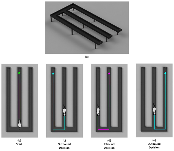
The behavioral apparatus (Figure 1 (a)) consists of an 150cm × 90cm acrylic track with three identical arms, each with a small food dish at the end. Infrared sensors along the track monitor the animals position and signal food reward delivery upon a correct arm visit using an Arduino microcontroller and a miniature inert liquid valve. Figure 1 (b-e) shows a schematic of the apparatus. Liquid food reward consisted of diluted vanilla nutrition shake (Ensure) and approximately 0.3 mL was administered upon every correct arm visit. Timestamps, correct/incorrect decisions, and position data were collected through a custom desktop application written in C#.
Figure 1. The W-Track Spatial Alternation Task.
TOP: (a) Schematic of the W-track apparatus. The 150cm × 90cm track has three identical arms. Liquid food rewards are dispensed into a food dish at the end of each arm. BOTTOM: Sequential illustration of correct performance on the W-track continuous spatial alternation task, demonstrating one possible sequence of arm visits that would result in a correct choice and a reward at every arm. (b) The animal starts at the center arm, facing the direction of the food dish at the end of the arm. An outbound decision (c and e) is considered to be any trial in which the rat departed from the center arm, while an inbound decision (d) is considered to be any trial in which the rat departed from either outside arm.
Behavioral Paradigm
Animals were first “pre-trained” to run for food rewards on a 150cm long linear track with a food dish at the end of each arm. The rat was required to walk the entire length of the track to receive a reward (this was considered a lap), and no reward was given for consecutive repeat visits to the same food dish. Rats were trained twice a day for 20 minutes until they were able to complete 30 laps in 20 minutes, at which point testing on the W-track began.
In each testing session, the animal had one hour to freely explore the track and to collect as many food rewards as they were able to retrieve. At the start of a session, the rat was first placed on the center arm, facing the direction of the food dish at the end of the arm (Figure 1b). After running to the end of the center arm and receiving a reward, the rat must then visit one of the outside arms (Figure 1c), return to the center (Figure 1d), and then visit the opposite outside arm (Figure 1e). The rat continues alternating between the outside arms, always returning to the center arm in-between each outbound trial. If, at any point, the animal makes an incorrect decision, they must return back to the center arm and resume the pattern.
Data Analysis
Individual Performance: State-Space Model.
Individual performance was measured using a state-space model applied to each animal’s performance (A. Smith et al., 2004). On each day, k, the observation for the jth animal is the number of correct responses, nj,k, in the mj,k trials performed during the one hour session. The individual performance for each rat is estimated using the state-space model described in detail in (A. Smith et al., 2004). Briefly, we assume each animal has an underlying cognitive state that is governed by a random walk. The model assumes the observations are binomial and computes the most likely cognitive state that fits the data via the Expectation-Maximization algorithm. From the cognitive state, it is then possible to compute a probability of a correct response for each animal.
A “learning session” (the session where the animal successfully acquired the task) was considered to be a session where the lower 90% confidence bound of the performance was above chance and remained above chance for the remaining trials in the testing period. Young and old animals’ learning session estimates were compared using the non-parametric Mann-Whitney U-test.
Group Performance: Repeated Measures ANOVA.
The first analysis method used to compare young and aged group performance is a repeated measures ANOVA. This is a commonly used approach that compares the differences between groups on measurements gathered sequentially. It tests the null hypothesis that our sample means come from the same population mean. The ANOVA analysis requires calculation of the variation across days, SStime the variation within group, SSwithin and the variation across subjects, SSsubjects. Each subject is treated as a level of an independent factor (i.e. each observation is independent and identically distributed, IID) and assumes the test variables follow a multivariate normal distribution.
We compute the sum of squares over time, SStime, from
| (1) |
where Jk is the total number of subjects the kth day, is the mean score of the kth day, , and is the grand mean and . The sum of squares for within subjects, SSwithin, is computed from:
| (2) |
Similarly, sum of squares for between subjects, SSsubjects, is
| (3) |
The sum of squares error, SSerror, is defined as
| (4) |
And the resulting F statistic for K days and J animals is computed:
| (5) |
Group Performance: Hierarchical Generalized Linear Model (GLM) and Hierarchical State-Space Model.
We present two alternative methods here: a hierarchical generalized linear model (model 1, GLM) and a hierarchical state-space model (model 2, SS).
Group performance can be well-characterized using a random effects or hierarchical modeling approach since this allows, via the exchangeability assumption, an accurate estimate of group variability. For our analysis we fit each group (young and aged) with a hierarchical GLM and hierarchical SS model, both described below. A Bayesian approach is used to estimate the model using the Python package PYMC3 (Python Software and Foundation. Python Language Reference (version 2.7) Available at http://www.python.org, 2010; Salvatier, Wiecki, & Fonnesbeck, 2016).
The observation model can be expressed as the binomial probability density function:
| (6) |
where the probability of a correct response, pj,k, relates to the state with a logistic function:
| (7) |
The parameter βj is unique to each animal and is assumed to be drawn from a normal distribution with zero mean and variance :
| (8) |
The variance describes the spread of the individuals about the group mean. For model 1 (GLM), we define the state by the linear equation:
| (9) |
where αj is a constant and ϵk is Gaussian random noise with zero mean and variance . For model 2 (SS) we define the state by the random walk:
| (10) |
Priors for both models are as follows:
| (11) |
| (12) |
and
| (13) |
Convergence was assessed by visual inspection of the time series of 1000 Monte Carlo estimates after an initial burn-in of 500 iterations was discarded.
Performance Comparison for Bayesian Models.
We use the Watanabe-Akaike Criterion (WAIC) (Watanabe, 2010) to compare model fits and predictive accuracy. The WAIC is a measure of the pointwise out-of-sample prediction accuracy from a fitted Bayesian model using the log-likelihood evaluated at the posterior simulations of the parameter values (Vehtari, Gelman, & Gabry, 2017). It is defined by
| (14) |
where is the computed log pointwise predictive density given by
| (15) |
and is the estimated effective number of parameters given by
| (16) |
Here, superscript s indicates the sth draw from the estimated posterior distributions and is the variance of the samples with respect to the mean.
RESULTS
Individual Performance Analysis
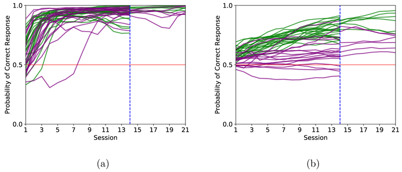
Figures 2 (a) and 2 (b) show the modes of the learning curves from a state-space analysis of each individual animal for inbound and outbound decisions, respectively, across the 14-day and 21-day testing protocols. With the exception of four old animals performing the shorter protocol, all animals’ performance tends to improve across time. It is also evident that for both young (green lines) and aged animals (purple lines), the inbound component (Figure 2a) of the task is learned more quickly than is the outbound component (Fig 2b). Figure 3 provides a summary of the learning trials computed from the lower 90% confidence bounds of the state-space model fits to each animal’s performance data for the two different length experiments considered separately.
Figure 2. Individual learning analysis through state-space analysis.
Each animal’s proportion of correct decisions were fit to a state-space model and the resulting learning curves for the inbound (a) and outbound (b) component of the task are plotted here for both the animals that completed 14 sessions and animals that completed 21 sessions. Young animals are plotted in green and old are in purple.
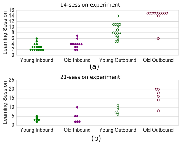
Figure 3. Summary of Learning Sessions.
(a) Learning sessions for animals that were tested for 14 sessions. Ten of the 12 aged animals were unable to learn the outbound component of the task in 14 sessions. (b) Learning sessions for animals that were tested for 21 sessions. All animals were able to learn the outbound component of the task with this extended testing paradigm.
Shorter 14 Day Testing Protocol.
For the inbound learning trials in the 14 day testing protocol the young animals learned significantly sooner than the old animals (Figure 3a, Mann-Whitney-U-test p = 0.03, U = 56.5; mean, μyoung = 3.0, standard deviation, σyoung = 1.17; mean, μold = 3.92, standard deviation, σold = 1.38). For the outbound component of the task, young animals learned approximately halfway through the testing period, whereas 10 of the 12 aged animals never learned this component of the task (Figure 3b). Assuming the learning trial for the animals that did not learn in 14 trials was 15, we find again that the two age groups were significantly different (Figure 3a, Mann-Whitney-U-test p < 0.001, U = 15.0; YOUNG: μyoung = 8.71, σyoung = 2.42; OLD: μold = 14.2, σold = 2.59]
Since learning in the outbound component was not observed in the aged animals, a second experiment was conducted with an extended testing period of 21 sessions.
Longer 21 day testing protocol.
The group that was tested over 21 sessions had similar inbound learning sessions as the first cohort though in this case the between-age group difference was not significant (Figure 3b, Mann-Whitney-U-test p = 0.5, U = 17.5; μyoung = 3.33, σyoung =1.03; μold = 4.33, σold = 3.14).
For the outbound group, all animals learned during the extended testing paradigm. The learning session for the outbound component is significantly later for older animals than young (Mann-Whitney-U-test p = 0.0099, U = 3.0, μyoung = 8.33, σyoung = 1.97; aged: μold = 16.0, σold = 4.65).
Group Performance Analysis
In order to accurately infer group statistics, three different analysis approaches were used: (1) repeated measures ANOVA, (2) hierarchical generalized linear model (GLM), and(3) hierarchical state-space.
Repeated Measures ANOVA.
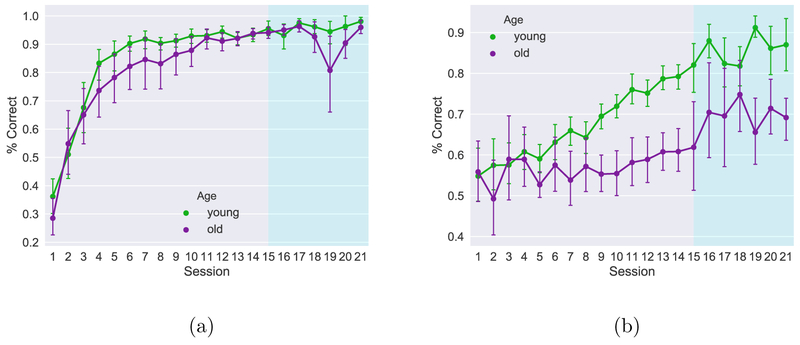
The average proportion of correct responses per session computed from the raw behavioral performance data is shown in Figure 4. The animals in the young group, on average, perform better than did those in the aged group (green lines > purple lines) and this age difference appears to be more pronounced in the outbound trials. The error bars are larger from session 15 onwards because the estimate is based on fewer observations. There is a tendency for both groups to perform slightly below chance at the beginning of the experiment on the inbound trials. We hypothesize that this is a result of pre-training on a linear track, as, during pre-training, animals are conditioned to run from one end of an arm to the other end without making any turns in the middle of their path. This may explain why both groups tend to make more inbound errors at the beginning of the testing period.
Figure 4. Mean task performance.
Average group performance with 95% confidence intervals on the inbound (a) and outbound(b) components of the task for all animals tested. The extended testing period for the 12 animals is shaded in blue. Mean performance was used for the repeated measures ANOVA.
We looked for age effects using a two-way ANOVA for repeated measures, a conventional method used in population learning studies. For the group with 14 testing sessions, younger animals performed better than old animals in the outbound part of the task (F(1,27) = 36.36, p < 0.0001) but not for the inbound component (F(1,27) = 2.74, p = 0.11). This was also true of the group that underwent extended testing (Inbound: F(1,12) = 1.53, p = 0.24 Outbound: F(1,12) = 31.44, p < 0.0001)
Hierarchical GLM and Hierarchical State-Space Random Effects Models.
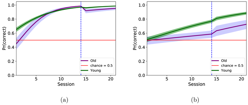
The second two approaches use hierarchical modeling. First, a hierarchical GLM was fit to the data (Figure 5) for both the 14-session and extended testing procedures. The young animals’ performance significantly exceeded the aged animals’ performance for the outbound part of the task, but was not significantly different for the inbound part of the task. The GLM also shows a greater separation of the groups, when compared to the mean performance data (Figure 4). It is clear that there is a separation of performance between the young and aged animals, but the learning curves do not look comparable to the raw data (Figure 4).
Figure 5. Hierarchical GLM analysis.
Results of the hierarchical GLM fit to data for inbound decisions (a) and outbound decisions (b).
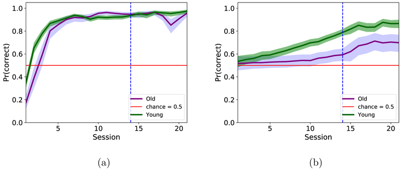
Second, a hierarchical state-space random effects model was fit to the data (Figure 6). Comparing the group learning curves with the GLM estimates, we see a general overall trend for the young to perform better than the aged do (green > purple). However, the state-space model has greater curvature, especially for the inbound trials which are learned more quickly.
Figure 6. Hierarchical state-space analysis.
Results of the hierarchical state-space random effects model fit to data for inbound decisions (a) and outbound decisions (b).
To assess which of the two hierarchical models best represents the data we looked at their respective WAICs (Table 1). In all cases, the WAIC of the hierarchical state-space model is lower than that of the hierarchical GLM, indicating better fit or representation of the data.
Table 1.
WAIC values for hierarchical models using 14-session-data (LEFT) and 21-session-data (RIGHT). In all cases, the Hierarchical State-Space model has a better fit than does the hierarchical GLM.
| Age | Trial Type | Model | WAIC | Age | Trial Type | Model | WAIC | |
|---|---|---|---|---|---|---|---|---|
| Young | Inbound | Hierarchical State Space | 162.81 | Young | Inbound | Hierarchical State-Space | 301.54 | |
| GLM | 345.16 | GLM | 430.90 | |||||
| Outbound | Hierarchical State-Space | 101.84 | Outbound | Hierarchical State-Space | 147.01 | |||
| GLM | 150.31 | GLM | 159.30 | |||||
| Aged | Inbound | Hierarchical State-Space | 216.42 | Aged | Inbound | Hierarchical State-Space | 283.74 | |
| GLM | 464.63 | GLM | 449.07 | |||||
| Outbound | Hierarchical State-Space | 89.33 | Outbound | Hierarchical State Space | 166.60 | |||
| GLM | 146.80 | GLM | 169.72 |
It is clear from Figure 6 that young animals learn the working memory-dependent part of this task significantly (outbound) faster and their performance remains above the performance of old animals throughout testing, even with additional testing sessions.
DISCUSSION
There were two primary novel findings that emerged from these experiments. First, aged rats made more errors throughout testing on the W-track spatial alternation task, requiring more days to reach learning criterion. In addition, aged animals remain below young rats’ performance on the outbound (working memory) component of the task, even with extended testing. The inbound component was not, however, substantially affected by age after learning criterion was met. Aged rats may be more impaired on the outbound part of the task because it required cooperation between the hippocampus and the mPFC, each of which is compromised with age, and when required to work together for task solution, may compound the performance deficit.
The deficits observed in aged rats on this task suggest impaired hippocampal-prefrontal interactions. There are at least two possible sources of these deficits, including altered synchrony across oscillatory networks in the hippocampus and the PFC (Jones & Wilson, 2005), impaired reactivation of behavioral experiences via awake or sleep sharp wave ripple events(Tang, Shin, Frank, & Jadhav, 2017), or a combination of these. To that end, future directions of this work should include performing simultaneous dual-region ensemble recordings from these two structures. A comparison of young and aged animals with both behavior and electrophysiology will provide a deeper insight into how age impacts network dynamics between these two regions. Additionally, these experiments may identify the source of wide variability in performance within both age groups, and may be particularly interesting in animals that demonstrate atypical behavioral performance for their age.
The second main finding of this study was that hierarchical state-space modeling appears to be the most effective analysis method for comparing young and old rats’ behavior on the W-track spatial alternation task. Although a state-space model analysis fit to each animal’s behavioral performance is sufficient for analyzing an individual’s learning over time and provides us with an idea of the distribution of performance, it does not allow session-by-session comparison of the two groups. To initially compare the learning of young and aged animals on this task, we performed a repeated measures ANOVA test, which is commonly used in experiments that measure an observation over time. While the repeated measures ANOVA did provide support for overall age differences on the task performance, this statistic was not helpful in identifying the subtle features of the learning differences between age groups.
To achieve a more fine grained evaluation of behavior differences, hierarchical modeling seemed well-suited because such models assume that observations from individuals come from the same underlying distribution, allowing us to detect individual differences without ignoring their inherent similarities. For that reason, we fit a hierarchal GLM and a hierarchical state-space model to the data and compared their fit to the raw behavioral data. Our assessment of the hierarchical GLM analysis is that it is too rigid to capture the curvature of the actual learning process. In practice, the hierarchical state-space model appears to be better suited to describe animal learning rates, as it is better able to capture the dynamics of the behavioral responses over time.
In summary, older rats made more errors overall and took longer to reach learning criterion on the W-track spatial alternation task than did younger rats. When the main component parts of the task were viewed independently, the old rats were the most impaired on the outbound, spatial working memory aspect of the task - the component that requires an interaction between prefrontal cortex and the hippocampal systems. The analytic tool that was most sensitive to these age differences was the hierarchical state-space model, which should prove extremely useful for analysis of complex behavioral data.
ACKNOWLEDGEMENTS
We would like to thank Jessica Brewster, Olivia Pietz, and Revathi Pillai with the assistance in the collection of data, as well as Michelle Albert, Luann Snyder, and Michael Montgomery for administrative support. We would also like to acknowledge software consultant, Daniel Kapellusch, for guidance in the creation of the custom-made W-Track desktop application for data collection.
This work was supported by the McKnight Brain Research Foundation and National Institutes of Health Grant R01 AG050548.
References
- Ando S, & Ohashi Y (1991). Longitudinal study on age-related changes of working and reference memory in the rat. Neuroscience Letters, 128(1), 17–20. [DOI] [PubMed] [Google Scholar]
- Barnes C (1979). Memory deficits associated with senescence: a neurophysiological and behavioral study in the rat. Journal of Comparative and Physiological Psychology, 93 (1), 74. [DOI] [PubMed] [Google Scholar]
- Bimonte H, Nelson M, & Granholm A-C (2003). Age-related deficits as working memory load increases: relationships with growth factors. Neurobiology of Aging, 24 (1), 37–48. [DOI] [PubMed] [Google Scholar]
- Birren J (1962). Age differences in learning a two-choice water maze by rats. Journal of Gerontology. [DOI] [PubMed] [Google Scholar]
- Delatour B, & Gisquest-Verrier P (1999). Lesions of the prelimbic-infralimbic cortices in rats do not disrupt response selection processes but induce delay-dependent deficits: evidence for a role in working memory? Behavioral Neuroscience, 113 (5), 941. [DOI] [PubMed] [Google Scholar]
- Ferino F, Thierry A, & Glowinski J (1987). Anatomical and electrophysiological evidence for a direct projection from ammon’s horn to the medial prefrontal cortex in the rat. Experimental Brain Research, 65(2), 421–426. [DOI] [PubMed] [Google Scholar]
- Frank L, Brown E, & Wilson M (2000). Trajectory encoding in the hippocampus and entorhinal cortex. Neuron, 27(1), 169–178. [DOI] [PubMed] [Google Scholar]
- Frick K, Baxter M, Markowska A, Olton D, & Price D (1995). Age-related spatial reference and working memory deficits assessed in the water maze. Neurobiology of Aging, 16(2), 149–160. [DOI] [PubMed] [Google Scholar]
- Gallagher M, & Rapp P (1997). The use of animal models to study the effects of aging on cognition. Annual Review of Psychology, 48(1), 339–370. [DOI] [PubMed] [Google Scholar]
- Gelman A, & Hill J (2006). Data analysis using regression and multilevel/hierarchical models. Cambridge university press. [Google Scholar]
- Goodrick C (1972). Learning by mature-young and aged wistar albino rats as a function of test complexity. Journal of Gerontology. [DOI] [PubMed] [Google Scholar]
- Granon S, & Poucet B (1995). Medial prefrontal lesions in the rat and spatial navigation: evidence for impaired planning. Behavioral Neuroscience, 109 (3), 474. [DOI] [PubMed] [Google Scholar]
- Jay T, Glowinski J, & Thierry A-M (1989). Selectivity of the hippocampal projection to the prelimbic area of the prefrontal cortex in the rat. Brain Research, 505(2), 337–340. [DOI] [PubMed] [Google Scholar]
- Jones M, & Wilson M (2005). Theta rhythms coordinate hippocampal-prefrontal interactions in a spatial memory task. PLoS biology, 3 (12), e402. [DOI] [PMC free article] [PubMed] [Google Scholar]
- Jung M, Qin Y, McNaughton B, & Barnes C (1998). Firing characteristics of deep layer neurons in prefrontal cortex in rats performing spatial working memory tasks. Cerebral Cortex, 8(5), 437–450. [DOI] [PubMed] [Google Scholar]
- Kim S, & Frank L (2009). Hippocampal lesions impair rapid learning of a continuous spatial alternation task. PLOS ONE, 4 (5), 1–13. [DOI] [PMC free article] [PubMed] [Google Scholar]
- Markowska A, Stone W, Ingram D, Reynolds J, Gold P, Conti L, ... Olton D (1989). Individual differences in aging: behavioral and neurobiological correlates. Neurobiology of Aging, 10(1), 31–43. [DOI] [PubMed] [Google Scholar]
- Morris R, Garrud P, Rawlins J, & O’Keefe J (1982). Place navigation impaired in rats with hippocampal lesions. Nature, 297(5868), 681. [DOI] [PubMed] [Google Scholar]
- Petrides M, & Milner B (1982). Deficits on subject-ordered tasks after frontal-and temporal-lobe lesions in man. Neuropsychologia, 20(3), 249–262. [DOI] [PubMed] [Google Scholar]
- Python software and foundation. python language reference (version 2.7) available at http://www.python.org (2010).
- Salvatier J, Wiecki T, & Fonnesbeck C (2016, April). Probabilistic programming in python using pymc3. PeerJ Computer Science, 2, e55. [DOI] [PMC free article] [PubMed] [Google Scholar]
- Smith A, Frank L, Wirth S, Yanike M, Hu D, Kubota Y, ... Brown E (2004). Dynamic analysis of learning in behavioral experiments. Journal of Neuroscience, 24 (2), 447–461. [DOI] [PMC free article] [PubMed] [Google Scholar]
- Smith A, Stefani M, Moghaddam B, & Brown E (2005). Analysis and design of behavioral experiments to characterize population learning. Journal of Neurophysiology, 93(3), 1776–1792. [DOI] [PubMed] [Google Scholar]
- Smith M, & Milner B (1981). The role of the right hippocampus in the recall of spatial location. Neuropsychologia, 19(6), 781–793. [DOI] [PubMed] [Google Scholar]
- Swanson L (1981). A direct projection from ammon’s horn to prefrontal cortex in the rat. Brain Research, 217(1), 150–154. [DOI] [PubMed] [Google Scholar]
- Tang W, Shin J, Frank L, & Jadhav S (2017). Hippocampal-prefrontal reactivation during learning is stronger in awake as compared to sleep states. Journal of Neuroscience, 2291–17. [DOI] [PMC free article] [PubMed] [Google Scholar]
- Vehtari A, Gelman A, & Gabry J (2017). Practical bayesian model evaluation using leave-one-out cross-validation and waic. Statistics and Computing, 27(5), 1413–1432. [Google Scholar]
- Wang G-W, & Cai J-X (2006). Disconnection of the hippocampal-prefrontal cortical circuits impairs spatial working memory performance in rats. Behavioural brain research, 175(2), 329–336. [DOI] [PubMed] [Google Scholar]
- Watanabe S (2010). Asymptotic equivalence of bayes cross validation and widely applicable information criterion in singular learning theory. Journal of Machine Learning Research, 11 (December), 3571–3594. [Google Scholar]


