Causality on longitudinal data: Stable specification search in constrained structural equation modeling

Abstract

A typical problem in causal modeling is the instability of model structure learning, i.e., small changes in finite data can result in completely different optimal models. The present work introduces a novel causal modeling algorithm for longitudinal data, that is robust for finite samples based on recent advances in stability selection using subsampling and selection algorithms. Our approach uses exploratory search but allows incorporation of prior knowledge, e.g., the absence of a particular causal relationship between two specific variables. We represent causal relationships using structural equation models. Models are scored along two objectives: the model fit and the model complexity. Since both objectives are often conflicting, we apply a multi-objective evolutionary algorithm to search for Pareto optimal models. To handle the instability of small finite data samples, we repeatedly subsample the data and select those substructures (from the optimal models) that are both stable and parsimonious. These substructures can be visualized through a causal graph. Our more exploratory approach achieves at least comparable performance as, but often a significant improvement over state-of-the-art alternative approaches on a simulated data set with a known ground truth. We also present the results of our method on three real-world longitudinal data sets on chronic fatigue syndrome, Alzheimer disease, and chronic kidney disease. The findings obtained with our approach are generally in line with results from more hypothesis-driven analyses in earlier studies and suggest some novel relationships that deserve further research.

1 Introduction

Causal modeling, an essential problem in many disciplines,^1–6 attempts to model the mechanisms by which variables relate and to understand the changes on the model if the mechanisms were manipulated.⁷ In the medical domain, revealing causal relationships may lead to improvement of clinical practice, for example, the development of treatment and medication. Slowly but steadily, causal discovery methods find their way into the medical literature, providing novel insights through exploratory analyses.^8–10 Moreover, data in the medical domain are often collected through longitudinal studies. Unlike in a cross-sectional design, where all measurements are obtained at a single occasion, the data in a longitudinal design consist of repeated measurements on subjects through time. Longitudinal data make it possible to capture change within subjects over time and thus gives some advantage to causal modeling in terms of providing more knowledge to establish causal relationships.¹¹ As emphasized in Fitzmaurice et al.,¹² there is much natural heterogeneity among subjects in terms of how diseases progress that can be explained by the longitudinal study design. Another advantage is that in order to obtain a similar level of statistical power as in cross-sectional studies, fewer subjects in longitudinal studies are required.¹³

To date, a number of causal modeling methods have been developed for longitudinal (or time series) data. Some of the methods are based on a Vector Autoregressive (VAR) and/or Structural Equation Model (SEM) framework which assumes a linear system and independent Gaussian noise.^14–18 Some other methods, interestingly, take advantage of nonlinearity,^19–21 or non-Gaussian noise,^20,22 to gain even more causal information. Most of the aforementioned methods conduct the estimation of the causal structures in somewhat similar ways. Bessler and Lee,¹⁵ Demiralp and Hoover,¹⁶ Moneta,¹⁷ Peters et al.,²⁰ Hyvärinen et al.²² use the (partial correlations of the) VAR residuals to either test independence or as input to a causal search algorithm, e.g., LiNGAM (linear non-Gaussian acyclic model),²³ PC (“P” stands for Peter, and “C” for Clark, the authors).²⁴ In general, these causal search algorithms are solely based on a single run of model learning which is notoriously unstable small changes in finite data samples can lead to entirely different inferred structures. This implies that some approaches might not be robust enough to correctly estimate causal models from various data, especially when the data set is noisy or has small sample size.

In the present paper, we introduce a robust causal modeling algorithm for longitudinal data that is designed to resolve the instability inherent to structure learning. We refer to our method as S3L, an abbreviation for stable specification search for longitudinal data. It extends our previous method,²⁵ here referred to as S3C, which is designed for cross-sectional data. S3L is a general framework which subsamples the original data into many subsets, and for each subset, S3L heuristically searches for Pareto optimal models using a multi-objective optimization approach. Among the optimal models, S3L observes the so-called relevant causal structures, which represent both stable and parsimonious model structures. These steps constitute the structure estimation of S3L which is fundamentally different from the aforementioned approaches that mostly use a single run for model estimation. For completeness, detail about S3C/L is described in Section 2. Moreover, in the default setting S3L assumes some underlying contexts: independent and identically distributed (iid) samples for each time slice (lag), linear system, additive independent Gaussian noise, causal sufficiency (no latent variables), stationary (time-invariant causal relationships), and fairly uniform time intervals between time slices.

The main contributions of S3L are:

• The causal structure estimation of S3L is conducted through multi-objective optimization and stability selection²⁶ over optimal models, to optimize both the stability and the parsimony of the model structures.

• S3C/L is a general framework which allows for other causal methods with all of their corresponding assumptions, e.g., nonlinearity, non-Gaussianity, to be plugged in as model representation and estimation. The multi-objective search and the stability selection part are independent of any mentioned assumptions.

• In the default model representation, S3L adopts the idea of the “rolling” model from Friedman et al.²⁷ to transform a longitudinal SEM model with an arbitrary number of time slices into two parts: a baseline model and a transition model. The baseline model captures the causal relationships at baseline observations, when subjects enter the study. The transition model consists of two time slices, which essentially represent the possible causal relationships within and across time slices. We also describe how to reshape the longitudinal data correspondingly, so as to match the transformed longitudinal model which then can easily be scored using standard SEM software.

• We provide standardized causal effects which are computed from Intervention-calculus when the DAG (directed acyclic graph) is Absent (IDA) estimates.²⁸

• We carry out experiments on three different real-world data of (a) patients with chronic fatigue syndrome (CFS), (b) patients with Alzheimer disease (AD), and (c) patients with chronic kidney disease (CKD).

Some relevant methods have attempted to make use of common structures to infer causal models. Causal stability ranking (CStaR),²⁹ originally designed for gene expression data, tries to find stable rankings of genes (covariates) based on their total causal effect on a specific phenotype (response), using a subsampling procedure similar to stability selection and IDA to estimate causal effects. As CStaR only focuses on relationships from all covariates to a single specific response, it seems to be difficult to generalize it to other domains where any possible causal relationship may be of interest. Moreover, another approach called group iterative multiple model estimation (GIMME),³⁰ originally developed for functional magnetic resonance imaging (fMRI) data and essentially an extension of extended unified SEM (combination of VAR and SEM),³¹ aims to combine the group-level causal structures with the individual-level structures, resulting in a causal model for each individual which contains common structures to the group. Such subject-specific estimation may be feasible given relatively long time series (as in resting state fMRI), but likely too challenging for the typical longitudinal data in clinical studies with a limited number of time slices per subject. Still in the domain of fMRI, there is a method called independent multiple-sample greedy equivalence search (IMaGES).³² The method is a modification of GES (described in the following paragraph), and designed to handle unexpected statistical dependencies in combined data. Since IMaGES was developed mainly for combining results of multiple data sets, we do not consider it further.

Having both the transformed longitudinal model and the reshaped data, we can run other alternative approaches which are designed for cross-sectional data and conduct comprehensive comparisons. Here, for evaluation of S3L, we generate simulated data and compare with some advanced constrained-based approaches such as PC-stable,³³ conservative PC (CPC),³⁴ CPC-stable,^33,34 and PC-Max.³⁵ All of these methods are extensions of the PC algorithm which in principle consists of two stages. The first stage uses conditional independence tests to obtain the skeleton (undirected edges) of the model, and the second stage orients the skeleton based on some rules, resulting in an essential graph or Markov equivalence class model (described in Section 2.1; for more details, see Chickering³⁶). We also compare with an advanced score-based algorithm called fast greedy equivalent search (FGES).³⁷ It is an extension of GES which in general starts with an empty (or sparse) model, and iteratively adds an edge (forward phase) which mostly increases the score until no more edge can be added. Then GES iteratively prunes an edge (backward phase) which does not decrease/improve the score until no more edge can be excluded.

The rest of this paper is organized as follows. All methods used in our approach are presented in Section 2. The results and the corresponding discussions are presented in Section 3. Finally, conclusion and future work are presented in Section 4.

2 Methods

2.1 Stable specification search for cross-sectional data

In Rahmadi et al.²⁵, we introduced our previous work, S3C, which searches over structures represented by SEMs. In SEMs, refining models to improve the model quality is called specification search. Generally, S3C adopts the concept of stability selection²⁶ in order to enhance the robustness of structure learning by considering a whole range of model complexities. Originally, in stability selection, this is realized by varying a continuous regularization parameter. Here, we explicitly consider different discrete model complexities. However, to find the optimal model structure for each model complexity is a hard optimization problem. Therefore, we rephrase stability selection as a multi-objective optimization problem, so that we can jointly run over the whole range of model complexities and find the corresponding optimal structures for each model complexity.

In more detail, S3C can be divided into two phases. The first phase is search, performing exploratory search over SEMs using a multi-objective evolutionary algorithm called Non-dominated Sorting Genetic Algorithm II (NSGA-II).³⁸ NSGA-II is an iterative procedure which adopts the idea of evolution. It starts with random models, and in every generation (iteration), attempts to improve the quality of the models by manipulating (refining) good models (parents) to make new models (offsprings). The quality of the models is characterized by scoring that is based on two conflicting objectives: model fit with respect to the data and model complexity. The model manipulations are realized by using two genetic operators: crossover that combines the structures of parents and mutation that flips the structures of models. Moreover, the composition of model population in the next generation is determined by selection strategy. One of the key features of NSGA-II is that in every iteration, it sorts models based on the concept of domination, yielding fronts or sets of models such that models in front l dominate those in front l + 1. The domination concept states that model m₁ is said to dominate model m₂ if and only if model m₁ is no worse than m₂ in all objectives and the model m₁ is strictly better than m₂ in at least one objective. The first front of the last generation is called the Pareto optimal set, giving optimal models for the whole range of model complexities. Details of the NSGA-II algorithm are described in Deb et al.³⁸

Based on the idea of stability selection,²⁶ S3C subsamples N subsets from the data D with size $\lfloor \left|D\right|/2\rfloor$ without replacement, and for each subset, the search phase above is applied, giving sets of Pareto optimal models. After that, all Pareto optimal models are transformed into their corresponding Markov equivalence classes which can be represented by completed partially directed acyclic graphs (CPDAGs).³⁶ Since all DAGs that are a member of the same Markov equivalence class represent the same probability distribution, they are indistinguishable based on the observational data alone. In SEMs, these models are called covariance equivalent³⁹ and return the same scores. From these CPDAGs, we compute the edge and causal path stability graphs (see Figure 7 for an example) by grouping them according to model complexity and computing their selection probability, i.e., the number of occurrences divided by the total number of models for a certain level of model complexity. The edge stability considers any edge between a pair of variables (i.e., $A\to B,B\to A$, or A–B) and the causal path stability considers directed path, e.g., $A\to B$ of any length. Stability selection is then performed by specifying two thresholds, ${\pi }_{\text{sel}}$ (boundary of selection probability) and ${\pi }_{\text{bic}}$ (boundary of complexity). For example, setting ${\pi }_{\text{sel}}=0.6$ means that all causal relationships with edge stability or causal path stability greater than or equal to this threshold are considered stable. The second threshold ${\pi }_{\text{bic}}$ is used to control overfitting. For every model complexity j, we compute the Bayesian information criterion (BIC) score for each model in j based on the data subset to which the model is fitted. We then compute ${\overline{\mathrm{BIC}}}_j$, the average of BIC scores in model complexity j. We set ${\pi }_{\text{bic}}$ to the minimum ${\overline{\mathrm{BIC}}}_j$. All causal relationships with an edge stability or a causal path stability that is smaller than or equal to ${\pi }_{\text{bic}}$ (e.g., ${\pi }_{\text{bic}}=27$ in Figure 7(c)) are considered parsimonious. Hence, the causal relationships greater than or equal to ${\pi }_{\text{sel}}$ and smaller than or equal to ${\pi }_{\text{bic}}$ are considered both stable and parsimonious and called relevant from which we can derive a causal model. In addition, we call the region with which the relevant structures intersect as relevant region.

Figure 7.

The stability graphs of the baseline model in (a) and (b) and the transition model in (c) and (d) for chronic fatigue syndrome, with edge stability in (a) and (c), and causal path stability in (b) and (d). The relevant regions, above ${\pi }_{\text{sel}}$ and left of ${\pi }_{\text{bic}}$, contain the relevant structures.

The second phase concerns visualization, combining the stability graphs into a graph with nodes and edges. This is done by adding the relevant edges and orienting them using prior knowledge (described in Section 2.2.2) and the relevant causal paths. More specifically, we first connect the nodes following the relevant edges. Then we orient these edges based on the prior knowledge. And finally, we orient the rest of the edges following the relevant causal paths of length one. The resulting graph consists of directed edges which represent causal relationship and possibly with additional undirected edges which represent strong association but for which the direction is unclear from the data. Furthermore, following Meinshausen and Bühlmann,²⁶ for each edge in the graph we take the highest selection probability it has across different model complexities in the relevant region of the edge stability graph as a measure of reliability and annotate the corresponding edge with this reliability score. The reliability score indicates the confidence of a particular relevant structure. The higher the score, the more we can expect that the relevant structure is not falsely selected.²⁶ In addition, each directed edge is annotated with a standardized causal effect estimate which is explained in Section 2.2.3. The stability graphs are considered to be the main outcome of our approach where the visualization eases interpretation.

2.2 S3L

S3L is an extension of S3C. In principle, as illustrated in Figure 1, S3L applies S3C on transformed longitudinal models, called baseline and transition models (explained in Section 2.2.1). Furthermore, in order to see to which extent a covariate would cause a response, S3L provides standardized total causal effect estimates which are intrinsically computed from estimates from IDA²⁸ (described in Section 2.2.3). In the following subsections, we first describe how we transform a longitudinal model and reshape the data accordingly, and then we discuss the implication of allowing prior knowledge in our S3C structure learning.

Figure 1.

Given a longitudinal data set, S3L uses the baseline observations to infer a baseline model, and reshapes the whole data set to infer a transition model. Both baseline and transition models are annotated with a reliability score α and a standardized causal effect β.

S3C: stable specification search for cross-sectional data; S3L: stable specification search for longitudinal data.

2.2.1 Longitudinal model and data reshaping

Based on the idea of a “rolling” network in Friedman et al.²⁷, we transform a longitudinal SEM with an arbitrary number of time slices (e.g., Figure 2(c)) into two parts: a baseline model (Figure 2(a)) and a transition model (Figure 2(b)). In the original paper, the authors treat these models as probabilistic networks, here we treat them purely as SEMs. The baseline model essentially represents the causal relationships between variables that may happen at the initial time slice t₀, for instance, causal relationships that occur before a medical treatment started. Moreover, the baseline model may also represent relationships of the unobserved process before t₀.²⁷ The transition model constitutes the causal relationships between variables across time slices $t_{i-1}$ and t_i, and between variables within time slice t_i for i > 0, for example, causal relationships that represent interactions during a medical treatment. In S3L, the structure estimations will be conducted on the baseline and transition model separately.

Figure 2.

(a) The baseline model which is used to capture causal relationships at the initial time slice, e.g., before medical treatment. (b) The transition model which is used to represent causal relationships within and between time slices, e.g., during medical treatment. (c) The corresponding “unrolled” longitudinal model.

From the transition model, we distinguish two kinds of causal relationships, namely intra-slice causal relationship (e.g., solid arcs in Figure 2(b)) and inter-slice causal relationship (e.g., dashed arcs in Figure 2(b)). The intra-slice causal relationship represents relationships within time slice t_i. Accordingly, the inter-slice causal relationship represents relationships between time slices $t_{i-1}$ and t_i. We assume that the inter-slice causal relationships are independent of t (stationary). We also assume that the time intervals between time slices are fairly uniform. In addition, the transition model implies two more constraints (explained in Section 2.2.2): there is no intra-slice causal relationship allowed in time slice $t_{i-1}$ and the inter-slice causal relationships always go forward in time, i.e., from time slice $t_{i-1}$ to time slice t_i.

Moreover, in order to score the transformed models, we reshape the longitudinal data accordingly. Figure 3 shows an illustration of the data reshaping. Suppose we are given longitudinal data with s instances, p variables, and i time slices, we assume that the original data shape is in a form of a matrix D of size s × q, with $q=p\times i$. The reshaped data is then a matrix $D\text{'}$ of size $s\text{'}\times q\text{'}$, with $s\text{'}=s(i-1)$ and $q\text{'}=2p$. Having such reshaped data allows us to use standard SEM software to compute the scores.

Figure 3.

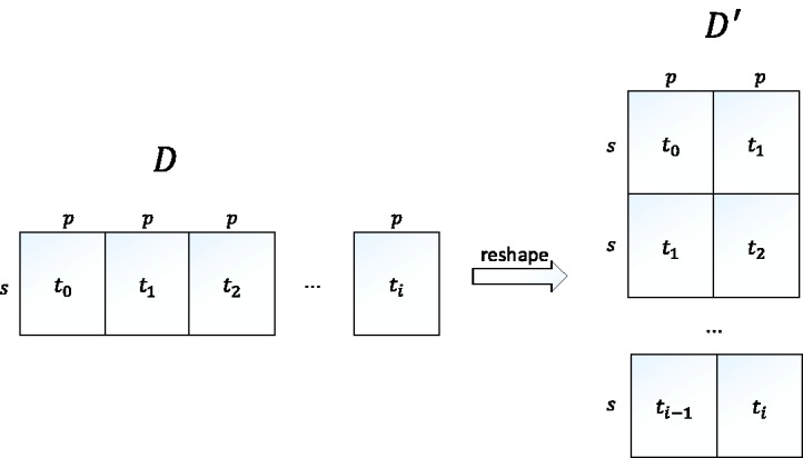
D is a matrix representing the original data shape which consists of s instances, p variables, and i time slices. $D\text{'}$ is a matrix representing the corresponding reshaped data.

2.2.2 Constrained SEM

In practice, we are often given some prior knowledge about the data. The prior knowledge which may be, e.g., results of previous studies, gives us some constraints in terms of causal relations. For example, in the case of, say disease A, there exists some common knowledge which tells us that symptom S does not cause disease A directly. In terms of a SEM specification, the prior knowledge can be translated into a constrained SEM in which there is no directed edge from variable S (denotes symptom S) to variable A (denotes disease A); this still allows for directed edges from A to S or directed paths (indirect relationships) from S to A, e.g., a path $S\to \dots \to A$ with any variables in between. S3C and hence S3L allow for such prior knowledge to be included in the model. In S3L, this prior knowledge only applies to the intra-slice causal relationships.

Model specifications should comply with any prior knowledge when performing specification search and when measuring the edge and causal path stability. Recall that in order to measure the stability, all optimal models (DAGs) are converted into their corresponding equivalence class models (CPDAGs). This model transformation, however, could result in CPDAGs that are inconsistent with the prior knowledge. For example, a constraint $A\neg \to B$ may be violated since arcs $B\to A$ in the DAG may be converted into undirected (reversible) edges A–B in the CPDAG. In order to preserve constraints, we therefore extended an efficient DAG-TO-CPDAG algorithm of Chickering,³⁶ as described in Rahmadi et al.²⁵ Essentially, the motivation of our extension to Chickering’s algorithm is similar to that of Meek’s algorithm,⁴⁰ that is, to obtain a CPDAG consistent with prior knowledge.

2.2.3 Estimating causal effects

We employ IDA²⁸ to estimate the total causal effects of a covariate X_i on a response Y from the relevant structures. This method works as follows. Given a CPDAG $G=\{G_1,\dots ,G_m\}$ which contains m different DAGs in its equivalence class, IDA applies intervention calculus^39,41 to each DAG G_j to obtain multisets ${\Theta }_i=\{{\theta }_{\mathrm{ij}}{\}}_{j\in 1,\dots ,m},i=1,\dots ,p$, where p is the number of covariates. θ_ij specifies the possible causal effect of X_i on Y in graph G_j.

Causal effects can be computed using the so-called intervention calculus,³⁹ which aims to determine the amount of change in a response variable Y when one would manipulate the covariate X_i (and not the other variables). Note that this notion differs from a regression-type of association (see IDA paper for illustrative examples). Given a DAG G_j, the causal effect θ_ij can be computed using the so-called back-door adjustment, which takes into account the associations between Y, X_i and the parents ${\text{pa}}_i(G_j)$ of X_i in G_j. Under the assumption that the distribution of the data is normal and the model is linear, causal effects can be computed from a regression of Y on X_i and its parents. Specifically, we have Maathuis et al.,²⁸ ${\theta }_{\mathrm{ij}}={\beta }_{i|{\text{pa}}_i(G_j)}$, where, for any set $S\subseteq \{X_1,\dots ,X_p,Y\}\setminus \{X_i\}$

$${\beta }_{i|S}=\{\begin{array}{ll}0,\hfill & \text{\hspace{0.17em}if\hspace{0.17em}}Y\in S\hfill \\ \text{\hspace{0.17em}coefficient\hspace{0.17em}of\hspace{0.17em}}{X}_i\text{\hspace{0.17em}in\hspace{0.17em}}Y\sim X_i+S,\hfill & \text{\hspace{0.17em}if\hspace{0.17em}}Y\cancel{\in }S\hfill \end{array}$$ (1)

and $Y\sim X_i+S$ is the linear regression of Y on X_i and S. Note that IDA estimates the total causal effect from a covariate to a response, which considers all possible, either direct or indirect, causal paths from the covariate to the response.

IDA works for continuous, normally distributed variables and then only requires their observed covariance matrix as input to compute the regression coefficients. Following Drasgow,⁴² we treat discrete variables as surrogate continuous variables, substituting the polychoric correlation for the correlation between two discrete variables and the polyserial correlation between a discrete and a continuous variable.

Our fitting procedure does not yield a single CPDAG, but a whole set of CPDAGs to represent the given data. We therefore extend IDA as follows. We gather $G_{{\pi }_{\text{bic}}}$, the CPDAGs of all optimal models with complexity equal to ${\pi }_{\text{bic}}$. For each CPDAG $G\in G_{{\pi }_{\text{bic}}}$, we compute the possible causal effects Θ of each relevant causal path using IDA. For example, for the causal effect from X to Y, we obtain estimates ${\Theta }_{X\to Y}^k,\hspace{1em}k=1,\dots ,N$, where N is the number of subsets. All causal effect estimations in ${\Theta }_{X\to Y}^k$ are then concatenated into a single multiset ${\Theta }_{X\to Y}$.

To represent the estimated causal effects from X to Y, we compute the median ${\tilde{\Theta }}_{X\to Y}$ and iff X and Y are continuous variables, we standardize the estimation using

$$\frac{{\tilde{\Theta }}_{X\to Y}·{\sigma }_X}{{\sigma }_Y}$$ (2)

where σ_X and σ_Y are the standard deviations of the covariate and the response, respectively. Standardized causal effects allow us to meaningfully compare them.

3 Results and discussion

3.1 Implementation

We implemented S3C and S3L as an R package named stablespec. The package is publicly available at the Comprehensive R Archive Network (CRAN) (https://cran.r-project.org/web/packages/stablespec/index.html), so it can be installed directly, e.g., from the R console by typing install.package(“stablespec”) or from RStudio. We also included a package documentation as a brief tutorial on how to use the functions.

3.2 Parameter settings

For application to simulated data and real-world data, we subsampled 50 and 100 subsets from the data with size $\lfloor \left|D\right|/2\rfloor$, respectively. We did not do comprehensive parameter tuning for NSGA-II, instead, we followed guidelines provided in Grefenstette.⁴³ The parameters for applications to both simulated and real-world data were set as follows: the number of iterations was 35, the number of models in the population was 150, the probability of applying crossover was 0.85, the probability of applying mutation to a model structure was 0.07, and the selection strategy was binary tournament selection.⁴⁴ We score models using the chi-square ${\chi }^2$ and the model complexity. The ${\chi }^2$ is considered the original fit index in SEM and measures how close the model-implied covariance matrix is to the sample covariance matrix.⁴⁵ The model complexity represents how many parameters (arcs) need to be estimated in the model. The maximum model complexity with p variables is given by $p(p-1)/2$.

When using multi-objective optimization we minimize both the ${\chi }^2$ and model complexity objectives. These two objectives are, however, conflicting with each other. For example, minimizing the model complexity typically means compromising the data fit.

3.3 Application to simulated data

3.3.1 Data generation

We generated data sets from a longitudinal model containing four continuous variables and three time slices (depicted by Figure 4). For each of sample sizes 400 and 2000, we generated 10 data sets with random parameterizations and made those publicly available (https://tinyurl.com/smmr-rahmadi-dataset).

Figure 4.

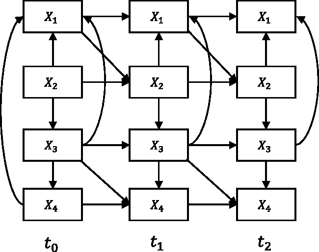
The longitudinal model with four variables and three time slices, used to generate simulated data.

3.3.2 Performance measure

We conducted comparisons between S3L with FGES, PC-stable, CPC, CPC-stable, and PC-Max in two different scenarios: with and without prior knowledge about part of the causal directions. Here, the comparisons focus more on the transition model, because in our previous paper²⁵ we already conducted experiments on the baseline model. In the case of prior knowledge, we added that variable X₁ at t_i cannot cause variables X₂ and X₃ at t_i directly. This prior knowledge translates to constraints that the various methods can use to restrict their search space. In addition to both scenarios, we also added longitudinal constraints to the models of FGES, PC-stable, CPC, CPC-stable, and PC-Max the same as those used in the transition model of S3L, i.e., there is no intra-causal relationship from time $t_{i-1}$ and the inter-slice causal relationships always go forward in time $t_{i-1}$ to t_i.

The parameters of FGES, PC-stable, CPC, CPC-stable, and PC-Max used in this simulation are set following some existing examples.^28,46,47 For FGES, the penalty of BIC score is 2 and the vertex degree in the forward search is not limited. For PC-stable, CPC, CPC-stable, and PC-Max, the significance level when testing for conditional independence is 0.01, and the maximum size of the conditioning sets is infinite.

Moreover, as the true model is known, we measure the performance of all approaches by means of the receiver operating characteristic (ROC)⁴⁸ for both edges and causal paths. We compute the true positive rate (TPR) and the false positive rate (FPR) based on the CPDAG of the true model. As for example, in the case of edge stability, a true positive means that an edge obtained by our method or the other approaches is present in the CPDAG of the ground truth.

To compare the ROC curves of our method and those of alternative approaches, we employed three significance tests. The first two tests, as introduced in DeLong et al.⁴⁹ and in Robin et al.,⁵⁰ compare the area under the curve (AUC) of the ROC curves by using the theory of U-statistics and bootstrap replicates, respectively. The third test, Venkatraman and Begg,⁵¹ compares the actual ROC curves by evaluating the absolute difference and generating rank-based permutations to compute the statistical significance. The null hypothesis is that (the AUC of) the ROC curves of our method and those of alternative approaches are identical.

Furthermore, we computed the ROC curves using two different schemes: averaging and individual. Both schemes are applied to all methods and to all data sets generated. In the averaging scheme, the ROC curves are computed from the average edge and causal path stability from different data sets, and then the statistical significance tests are applied to these ROC curves. On the other hand, in the individual scheme the ROC curves are computed from the edge and causal path stability on each data set. We then applied individual statistical significance tests on the ROC curves for each data set and used Fisher’s method,^52,53 to combine these test results into a single test statistic.

The experimental designs (with and without prior knowledge) and the ROC schemes (averaging and individual) are aimed to show empirically and comprehensively how robust the results are of each approach in various practical cases as well as against changes in the data.

3.3.3 Discussion

We first discuss the result of our experiments on the data set with sample size 400. Figure 5 shows the ROC curves for the edge stability (panels (a) and (c)) and the causal path stability (panels (b) and (d)) from the averaging scheme. Panels (a) and (b) represent the results without prior knowledge, while panels (c) and (d) represent the results with prior knowledge. Table 1 lists the corresponding AUCs.

Figure 5.

Results from simulation data with sample size 400: ROC curves for (a) the edge stability and (b) the causal path stability (without prior knowledge), and (c) the edge path stability and (d) the causal path stability (with prior knowledge), for different values of ${\pi }_{\text{sel}}$ in the range of $[0,1]$. Table 1 lists the corresponding AUCs.

CPC: conservative PC; FGES: fast greedy equivalent search; FPR: false positive rate; S3L: stable specification search for longitudinal data; TPR: true positive rate.

Table 1.

AUCs for the edge and causal path stability for each method, from simulation on data with sample size 400, with (yes) and without prior knowledge (no).

	S3L		FGES		PC-stable		CPC		CPC-stable		PC-Max
AUC	No	Yes	No	Yes	No	Yes	No	Yes	No	Yes	No	Yes
Edge	0.80	0.74	0.83	0.81	0.63	0.60	0.63	0.62	0.63	0.65	0.63	0.65
Causal	0.92	0.96	0.90	0.93	0.84	0.90	0.92	0.89	0.78	0.84	0.85	0.85

AUC: area under the curve; CPC: conservative PC; FGES: fast greedy equivalent search; S3L: stable specification search for longitudinal data.

Tables 2 and 3 present the results of the significance tests for both the averaging and individual schemes in the experiment with and without prior knowledge, respectively. In the case without prior knowledge, generally the AUCs of the edge and the causal path stability of S3L are better (p-value $\le 0.05$, or even $\le 0.001$, few of them are marginally significant, e.g., p-value $\le 0.1$) than those of other approaches according to both schemes, except those of FGES for which generally there is no evidence of a difference (p-value > 0.1). In the case with prior knowledge, in general the results are similar to those of experiment without prior knowledge, but now the AUC of the causal path stability of S3L is better (p-value $\le 0.05$) than that of FGES. The ROC of the causal path stability of S3L is now also better (p-value $\le 0.05$) than those of PC-stable, CPC, CPC-stable, and PC-Max according to the individual scheme. This is an improvement over the experiment without prior knowledge.

Table 2.

p-Values from comparisons on data set with sample size 400 between S3L and alternative approaches without prior knowledge.

		FGES		PC-stable		CPC		CPC-stable		PC-Max
Significance test		Avg.	Ind.	Avg.	Ind.	Avg.	Ind.	Avg.	Ind.	Avg.	Ind.
DeLong et al.48	Edge	0.315	0.909	0.021	<10−5	0.025	<10−5	0.052	<10−5	0.050	<10−5
	Causal	0.451	0.109	0.069	<10−5	0.825	<10−5	0.012	<10−5	0.126	<10−5
Robin et al.49	Edge	0.331	0.935	0.020	<10−5	0.024	<10−5	0.051	<10−5	0.049	<10−5
	Causal	0.466	0.090	0.063	<10−5	0.830	<10−5	0.010	<10−5	0.121	<10−5
Venkatraman and Begg50	Edge	0.304	0.906	0.091	0.102	0.076	0.118	0.359	0.516	0.449	0.743
	Causal	0.332	0.197	0.831	0.225	0.845	0.365	0.569	0.512	0.584	0.131

Note: The null hypothesis is that (the AUC of) the ROC curves of S3L and those of alternative approaches are equivalent. For each significance test, we compared the ROC of the edge (Edge) and causal path (Causal) stability (see Figure 5(a) and (b)) on both averaging (Avg.) and individual (Ind.) schemes.

AUC: area under the curve; CPC: conservative PC; FGES: fast greedy equivalent search; ROC: receiver operating characteristic.

Table 3.

p-Values from comparisons on data set with sample size 400 between S3L and alternative approaches with prior knowledge.

		FGES		PC-stable		CPC		CPC-stable		PC-Max
Significance test		Avg.	Ind.	Avg.	Ind.	Avg.	Ind.	Avg.	Ind.	Avg.	Ind.
DeLong et al.48	Edge	0.090	0.146	0.086	<10−3	0.099	<10−5	0.219	0.001	0.227	0.002
	Causal	0.264	0.003	0.061	<10−5	0.035	<10−5	0.022	<10−5	0.031	<10−5
Robin et al.49	Edge	0.118	0.188	0.084	<10−5	0.099	<10−5	0.208	<10−3	0.223	0.001
	Causal	0.251	0.002	0.060	<10−5	0.031	<10−5	0.020	<10−5	0.026	<10−5
Venkatraman and Begg50	Edge	0.430	0.598	0.056	0.680	0.103	0.543	0.680	0.998	0.707	0.998
	Causal	0.637	0.783	0.485	0.004	0.069	<10−3	0.116	0.094	0.171	0.007

Note: The null hypothesis is that (the AUC of) the ROC curves of S3L and those of alternative approaches are equivalent. For each significance test, we compared the ROC of the edge (Edge) and causal path (Causal) stability (see Figure 5(c) and (d)) on both averaging (Avg.) and individual (Ind.) schemes.

AUC: area under the curve; CPC: conservative PC; FGES: fast greedy equivalent search; ROC: receiver operating characteristic.

Next we discuss the result of our experiments on the data set with sample size 2000. Figure 6 shows the ROC curves and Table 4 lists the corresponding AUCs. Tables 5 and 6 list the results of the significance tests for both the averaging and individual schemes in the experiment with and without prior knowledge, respectively. In the case without prior knowledge, generally the AUCs of the edge and the causal path stability of S3L are better than (p-value $\le 0.05$) those of other approaches according to the individual scheme. Moreover, the ROCs of the edge and the causal path stability of S3L are better than those of FGES (p-value $\le 0.001$) and CPC-stable (p-value $\le 0.1$), respectively, according to the individual scheme. In the case with prior knowledge, the results are pretty much similar to those of the experiment without prior knowledge, but only now the p-value tends to become smaller, e.g., p-value $\le 0.001$.

Figure 6.

Results from simulation data with sample size 2000: ROC curves for (a) the edge stability and (b) the causal path stability (without prior knowledge), and (c) the edge path stability and (d) the causal path stability (with prior knowledge), for different values of ${\pi }_{\text{sel}}$ in the range of $[0,1]$. Tables 4 lists the corresponding AUCs.

CPC: conservative PC; FGES: fast greedy equivalent search; FPR: false positive rate; S3L: stable specification search for longitudinal data; TPR: true positive rate.

Table 4.

AUCs for the edge and causal path stability for each method, from simulation on data with sample size 2000, with (yes) and without prior knowledge (no).

	S3L		FGES		PC-stable		CPC		CPC-stable		PC-Max
AUC	No	Yes	No	Yes	No	Yes	No	Yes	No	Yes	No	Yes
Edge	0.77	0.73	0.77	0.78	0.67	0.67	0.69	0.65	0.62	0.61	0.65	0.60
Causal	0.92	0.93	0.85	0.90	0.90	0.94	0.88	0.93	0.87	0.87	0.92	0.91

AUC: area under the curve; CPC: conservative PC; FGES: fast greedy equivalent search; S3L: stable specification search for longitudinal data.

Table 5.

p-Values from comparisons on data set with sample size 2000 between S3L and alternative approaches without prior knowledge.

		FGES		PC-stable		CPC		CPC-stable		PC-Max
Significance test		Avg.	Ind.	Avg.	Ind.	Avg.	Ind.	Avg.	Ind.	Avg.	Ind.
DeLong et al.48	Edge	1.000	0.099	0.223	0.010	0.320	0.014	0.071	0.001	0.118	0.009
	Causal	0.052	<10−5	0.563	<10−3	0.353	<10−5	0.221	<10−5	0.952	0.183
Robin et al.49	Edge	1.000	0.103	0.222	0.007	0.321	0.010	0.077	0.003	0.103	0.006
	Causal	0.045	<10−5	0.554	<10−3	0.357	<10−5	0.202	<10−5	0.952	0.161
Venkatraman and Begg50	Edge	0.480	0.963	0.187	0.801	0.212	0.872	0.069	0.900	0.100	0.972
	Causal	0.418	<10−3	0.404	0.637	0.289	0.339	0.726	0.897	0.520	0.250

Note: The null hypothesis is that (the AUC of) the ROC curves of S3L and those of alternative approaches are equivalent. For each significance test, we compared the ROC of the edge (Edge) and causal path (Causal) stability (see Figure 6(a) and (b)) on both averaging (Avg.) and individual (Ind.) schemes.

AUC: area under the curve; CPC: conservative PC; FGES: fast greedy equivalent search; ROC: receiver operating characteristic.

Table 6.

p-Values from comparisons on data set with sample size 2000 between S3L and alternative approaches with prior knowledge.

		FGES		PC-stable		CPC		CPC-stable		PC-Max
Significance test		Avg.	Ind.	Avg.	Ind.	Avg.	Ind.	Avg.	Ind.	Avg.	Ind.
DeLong et al.48	Edge	0.296	0.978	0.413	<10−3	0.348	0.005	0.147	<10−3	0.122	<10−3
	Causal	0.142	<10−5	0.817	<10−3	0.698	<10−3	0.043	<10−5	0.279	<10−5
Robin et al.49	Edge	0.295	0.983	0.412	<10−3	0.344	0.002	0.146	<10−5	0.125	<10−5
	Causal	0.144	<10−5	0.833	<10−3	0.706	<10−3	0.043	<10−5	0.279	<10−5
Venkatraman and Begg50	Edge	0.761	0.862	0.119	0.207	0.210	0.290	0.146	0.082	0.140	0.257
	Causal	0.486	0.595	0.384	0.763	0.172	0.742	0.488	0.984	0.652	0.903

Note: The null hypothesis is that (the AUC of) the ROC curves of S3L and those of alternative approaches are equivalent. For each significance test, we compared the ROC of the edge (Edge) and causal path (Causal) stability (see Figure 6(c) and (d)) on both averaging (Avg.) and individual (Ind.) schemes.

AUC: area under the curve; CPC: conservative PC; FGES: fast greedy equivalent search; ROC: receiver operating characteristic.

To conclude, we see that in general S3L attains at least comparable performance as, but often a significant improvement over, alternative approaches. This holds in particular for causal directions and in the case of a small sample size. The presence of prior knowledge enhances the performance of the S3L.

3.4 Application to real-world data

Here the true model is unknown, so we can only compare the results of S3L with those reported in earlier studies and interpretation by medical experts. We set the thresholds to ${\pi }_{\text{sel}}=0.6$ and ${\pi }_{\text{bic}}$ to the model complexity where the minimum average of BIC scores is found. By thresholding we get the relevant causal relationships: those which occur in the relevant region. Details of the procedure are given in Section 2.1.

The model assumptions in the application to real-world data follow from the assumptions of S3L in the default setting. The assumptions include iid samples on each time slice, linear system, independent Gaussian noise, no latent variables, stationary, and fairly uniform time intervals between time slices.

Moreover, there is an important note related to the visualization of the stability graphs. A DAG without edges will always be transformed into a CPDAG without edges. A fully connected DAG without prior knowledge will be transformed into a CPDAG with only undirected edges. However, if prior knowledge is added, a fully connected DAG will be transformed into a CPDAG in which the edges corresponding to the prior knowledge are directed. From these observations, it follows that in the edge stability graph all paths start with a selection probability of 0 and end up in a selection probability of 1. In the causal path stability graph when no prior knowledge has been added, all paths start with a selection probability of 0 and end up in a selection probability of 0. However, when prior knowledge is added, some of the paths may end up in a selection probability of 1 because of the added constraints.

3.4.1 Application to CFS data

Our first application to real-world data considers a longitudinal data set of 183 patients with CFS who received cognitive behavior therapy (CBT).⁵⁴ Empirical studies have shown that CBT can significantly reduce fatigue severity. In this study, we focus on the causal relationships between cognitions and behavior in the process of reducing subject’s fatigue severity. We therefore include six variables namely fatigue severity, the sense of control over fatigue, focusing on the symptoms, the objective activity of the patient (oActivity), the subject’s perceived activity (pActivity), and the physical functioning. The data set consists of five time slices where the first and the fifth time slices are the pre- and post-treatment observations, respectively, and the second until the fourth time slices are observations during the treatment. The missing data are 8.7%, and to impute the missing values, we used single imputation with expectation maximization (EM) in SPSS.⁵⁵ As all of the variables have large scales, e.g., in the range between 0 and 155, we treat them as continuous variables. We added prior knowledge that the variable fatigue at t₀ and t_i does not cause any of the other variables directly. This is a common assumption made in the analysis of CBT in order to investigate the causal impact on fatigue severity.^54,56

First we discuss the baseline model, which only considers the baseline causal relationships. The corresponding stability graphs can be seen in Figure 7(a) and (b). As mentioned before, ${\pi }_{\text{sel}}$ is set to 0.6 and from the search phase of S3L we found that ${\pi }_{\text{bic}}=6$. Figure 7(a) and (b) shows that three relevant edges and two relevant causal paths were found. Following the visualization procedure (see visualization phase in Section 2.1), we get a baseline model in Figure 8(a). The model shows that pActivity is a direct cause for fatigue severity. This follows from the prior assumption that we made and is consistent with earlier works.^54,56 This causal relationship suggests that a reduction of (perceived) activity leads to an increase of fatigue. In addition, we found a strong relationship between pActivity and oActivity whose direction cannot be determined. This relationship is somewhat sensible as both variables measuring patient’s activity. We also found a connection between focusing and control, which is not surprising as focusing on symptoms also depends on patient’s sense of control over fatigue. One would expect that if a patient has less control on the fatigue, the focus on the symptom would increase.

Figure 8.

(a) The baseline model and (b) the transition model of chronic fatigue syndrome. The dashed line represents a strong relation between two variables but the causal direction cannot be determined from the data. Each edge has a reliability score (the highest selection probability in the relevant region of the edge stability graph) and a standardized total causal effect estimation. For example, the annotation “$1/0.71$“ represents a reliability score of 1 and a standardized total causal effect of 0.71. Note that the standardized total causal effect represents not just the direct causal effect corresponding to the edge, but the total causal effect also including indirect effects.

Next we discuss the transition model, which considers all causal relationships over time slices. The corresponding stability graphs are depicted in Figure 7(c) and (d). We set ${\pi }_{\text{sel}}=0.6$ and the search phase of S3L yielded ${\pi }_{\text{bic}}=27$. Figure 7(c) shows that 19 relevant edges were found, consisting of 11 intra-slice (blue lines) and 8 inter-slice relationships of which 6 are between the same variables (orange lines) and 2 are between different variables (black lines). Figure 7(d) shows that 35 relevant causal paths were found, consisting of 12 intra-slice (blue lines) and 23 inter-slice relationships of which 6 are between the same variables (orange lines) and 17 are between different variables (black lines). Applying the visualization procedure, we get the transition model in Figure 8(b). The model shows that all variables have intra-slice causal relationships to fatigue severity. These relationships are consistent with Vercoulen et al.,⁵⁶ Heins et al.,⁵⁴ and Wiborg et al.,⁵⁷ which conclude that during the CBT, an increase in sense of control over fatigue, physical functioning, and perceived physical activity, together with a decrease in focusing on symptoms lead to a lower level of fatigue severity. Interestingly, the actual activity seems insufficient to reduce fatigue severity⁵⁴; however, how the patient perceives his own activity does seem to help. Additionally, we also found that, with similar causal effects, all variables (except pActivity and fatigue) also cause the change in fatigue indirectly via pActivity as an intermediate variable. This suggests that, as discussed in Heins et al.,⁵⁴ an increase in perceived activity does seem important to explain the change in fatigue. The variables focusing and functioning also appear to be indirect causes of changes in the level of fatigue severity.

3.4.2 Application to AD data

For the second application to real-world data, we consider a longitudinal data set about AD, which is provided by the Alzheimer’s Disease Neuroimaging Initiative (ADNI),⁵⁸ and can be accessed at adni.loni.usc.edu. The ADNI was launched in 2003 as a public–private partnership, led by Principal Investigator Michael W Weiner, MD. The primary goal of ADNI has been to test whether serial magnetic resonance imaging, positron emission tomography, other biological markers, and clinical and neuropsychological assessment can be combined to measure the progression of mild cognitive impairment (MCI) and early AD. For up-to-date information see www.adni-info.org.

In the present paper, we focus on patients with MCI, an intermediate clinical stage in AD.⁵⁹ Following Haight and Jagust⁶⁰ we include only the variables: subject’s cognitive dysfunction (ADAS-Cog), hippocampal volume (hippocampal_vol), whole brain volume (brain_vol), and brain glucose metabolism (brain_glucose). The data set contains 179 subjects with four continuous variables and six time slices. The first time slice captures baseline observations and the next time slices are for the follow-up observations. The missing data are 22.9%, and as in the application to CFS, we imputed the missing values using single imputation with EM. We added prior knowledge that the variable ADAS-Cog at t₀ and t_i does not cause any of the other variables directly. We performed the search over 100 subsamples of the original data set.

First we discuss the baseline model which only considers the baseline causal relationships. The corresponding stability graphs are shown in Figure 9(a) and (b). ${\pi }_{\text{sel}}$ is set to 0.6 and the search phase of S3L found that ${\pi }_{\text{bic}}=4$. Figure 9(a) and (b) shows that four relevant edges and two relevant causal paths were found. Following the visualization procedure, we obtain the baseline model in Figure 10(a). We found that an increase in both brain glucose metabolism and hippocampal volume causes reduction in subject’s cognitive dysfunction. These causal relations are consistent with findings in Haight and Jagust⁶⁰ which also concluded that both brain_glucose and hippocampal_vol were independently related to ADAS-Cog (in our model, it is represented by independent direct causal paths). Additionally, strong relations between hippocampal volume and brain volume seem plausible as they both measure the volume of the brain (partly and entirely).

Figure 9.

The stability graphs of the baseline model in (a) and (b) and the transition model in (c) and (d) for Alzheimer’s disease, with edge stability in (a) and (c), and causal path stability in (b) and (d). The relevant regions, above ${\pi }_{\text{sel}}$ and left of ${\pi }_{\text{bic}}$, contain the relevant structures.

Figure 10.

(a) The baseline model and (b) the transition model of Alzheimer’s disease. The dashed line represents a strong relation between two variables but the causal direction cannot be determined from the data. Each edge has a reliability score (the highest selection probability in the relevant region of the edge stability graph) and a standardized total causal effect estimation. For example, the annotation “$1/0.81$“ represents a reliability score of 1 and a total standardized causal effect of 0.81. Note that the standardized total causal effect represents not just the direct causal effect corresponding to the edge, but the total causal effect also including indirect effects.

Next we discuss the transition model which considers all causal relationships across time slices. We set ${\pi }_{\text{sel}}=0.6$ and the search phase of S3L yielded ${\pi }_{\text{bic}}=12$. The corresponding stability graphs can be seen in Figure 9(c) and (d). We found 12 relevant edges (see Figure 9(c)), consisting of 4 intra-slice (blue lines) and 8 inter-slice relationships of which 4 are between the same variables (orange lines) and 4 are between different variables (black lines). Moreover, we found 17 relevant causal paths (see Figure 9(d)), consisting of 6 intra-slice (blue lines) and 11 inter-slice relationships of which 4 are between the same variables (orange lines) and 7 are between different variables (black lines). Applying the visualization procedure, we obtain the transition model in Figure 10(b). In addition, the direction of the edge from brain_glucose to brain_vol follows because we do not allow cycles in our model. We found that there are indirect and direct causal relationships from hippocampal_vol and brain_vol at both $t_{i-1}$ and t_i to ADAS-Cog at t_i. These particular causal relationships support the hypothesis in Haight and Jagust⁶⁰ which says that any changes in both hippocampal volume and brain volume will cause short-term effects on a subject’s cognitive dysfunction, both direct and indirect. In the original paper, the authors suggested that the indirect causal relationship is through brain_glucose, but our analysis also discovers a potential indirect effect through brain_vol. Interestingly, we found that a change in subject’s cognitive dysfunction in a previous time slice $t_{i-1}$ causes a reduction in brain volume in time slice t_i.

3.4.3 Application to CKD data

For the third application to real-world data, we consider a longitudinal data set about CKD, provided by the MASTERPLAN Study Group.⁶¹ The MASTERPLAN study was initiated in 2004 as a randomized, controlled trial studying the effect of intensified treatment with the aid of nurse practitioners on cardiovascular and kidney outcome in CKD. This intensified treatment regimen addressed 11 possible risk factors for the progression of CKD simultaneously. The study previously showed that this intensified treatment resulted in fewer patients reaching end-stage kidney disease compared to standard treatment.⁶¹

Here we focus on the potential causal mediators for the protective effect incurred by the intensified treatment with the aid of nurse practitioners. In other words, we aim to identify which of the treatment targets contributed to the observed overall treatment effect. In the present analysis, we include only variables of interest, being treatment status, either nurse practitioner aided care or standard care, as allocated by the randomization procedure (treatment), estimated glomerular filtration rate (gfr—a marker for overall kidney function), and a variable indicating informative censoring (inf_cens). Informative censoring occurred when patients reached end-stage kidney disease requiring renal replacement therapy, such as dialysis or a kidney transplantation, or when they died. Furthermore, we considered treatment targets that were previously hypothesized to contribute most to the overall treatment effect: systolic blood pressure (sbp), LDL-cholesterol (ldl) and parathyroid hormone (pth) concentrations in blood, and protein excretion via urine (pcr). In total, there are 497 subjects with 7 variables (both continuous and discrete) over 5 time slices. The first time slice contains the baseline observations taken before treatment, and the next time slices are the follow-up observations during treatment. Particularly, we set the variable treatment only at $t_{i-1}$ as it remains the same over all time slices, and the variable inf_cens only at t_i as it is a consequence of previous treatment. We further added the prior knowledge that gfr at t_i does not directly cause any other variables, and that there are no relations between any variable and inf_cens within t_i. Both gfr and inf_cens are read-out for CKD progression and are within a time slice always the consequence and never the cause of another variable. However, we relax this prior knowledge at time slice t₀ as it is a common assumption that without the treatment, pth is a consequence of poor kidney function. The missing data are 5.2%, and a single imputation with EM was conducted to impute the missing values like in applications to CFS and ADNI data. We performed the search over 100 subsamples of the original data set.

First we discuss the baseline model, which only considers the baseline causal relationships. Figure 11(a) and (b) depicts the corresponding stability graphs. As in applications to CFS and ADNI data, π_sel is set to 0.6 and based on the search phase of S3L we found that ${\pi }_{\mathrm{bic}}=2$. Figure 11(a) and (b) shows that two relevant edges were found. Applying the visualization procedure, we get the baseline model in Figure 12(a). We found that both pth and pcr were associated with kidney function at baseline. The direction of these associations remains unclear. From renal physiology, we know that proteinuria may result in kidney damage. However, kidney damage and proteinuria may be common consequences of hypertension at an earlier stage in the patient’s history. The association between parathyroid hormone and GFR is unsurprising, as calcium and phosphate metabolism is disrupted in patients with advanced kidney disease. However, elevated pth may in turn result in further kidney damage by increased vascular calcification. In other words, the associations seem plausible from a physiological point of view, but the association may be in either direction. In the CKD example, a causal direction is almost impossible to ascertain when only using cross-sectional data.

Figure 11.

The stability graphs of the baseline model in (a) and (b) and the transition model in (c) and (d) for chronic kidney disease, with edge stability in (a) and (c), and causal path stability in (b) and (d). The relevant regions, above ${\pi }_{\text{sel}}$ and left of ${\pi }_{\text{bic}}$, contain the relevant structures.

Figure 12.

(a) The baseline model and (b) the transition model of chronic kidney disease. The dashed line represents a strong relation between two variables but the causal direction cannot be determined from the data. Each edge has a reliability score (the highest selection probability in the relevant region of the edge stability graph) and a standardized total causal effect estimation. For example, the annotation “$1/0.88$” represents a reliability score of 1 and a standardized total causal effect of 0.88. Note that the standardized total causal effect represents not just the direct causal effect corresponding to the edge, but the total causal effect also including indirect effects.

Next we discuss the transition model, which takes into account all causal relationships across time slices. We set ${\pi }_{\text{sel}}=0.6$ and found ${\pi }_{\text{bic}}=23$. Based on Figure 11(c), we obtained 17 relevant edges, consisting of 4 intra-slice (blue lines) and 13 inter-slice relationships of which 5 are between the same variables (orange lines) and 8 are between different variables (black lines). Based on Figure 11(d), we obtained 26 relevant causal paths, consisting of 5 intra-slice (blue lines) and 21 inter-slice relationships of which 5 are between the same variables (orange lines) and 16 are between different variables (black lines). Applying the visualization procedure, we get the transition model in Figure 12(b). Most of the intra-slice and inter-slice causal relationships are very stable with selection probabilities close to 1. We found inter-slice causal relationships from gfr, sbp, pth, and pcr to inf_cens. Furthermore, gfr, sbp, and pcr are well-known determinants for CKD progression. The causal relationship from pth to inf_cens was somewhat surprising. However, pth is a marker for regulation of phosphate stores in the body and related to overall vascular damage through vascular calcification, and may thereby be related to mortality. Indeed, the literature indicates that lowering pth in dialysis patients resulted in a reduction in mortality.⁶² The same may hold true for patients who have CKD and who do yet need dialysis treatment. Perhaps most surprising are the relations between sbp and pcr and gfr, respectively. From renal physiology, we know that higher filtration pressure due to higher blood pressure causes the short-term glomerular filtration rate to increase slightly.⁶³ Likewise, at higher filtration pressure, more and larger proteins are pushed out of the blood stream and into the pro-urine and are ultimately excreted via the urine. In the long term, chronically elevated filtration pressures and elevated levels of protein in the pro-urine cause kidney damage and ultimately even end-stage kidney disease. Overall, the results are consistent with the literature and physiology.⁶⁴

4 Conclusion and future work

Causal discovery from longitudinal data turns out to be an important problem in many disciplines. In the medical domain, revealing causal relationships from a given data set may lead to improvement of clinical practice, e.g., further development of treatment and medication. In the past decades, many causal discovery algorithms have been introduced. These causal discovery algorithms, however, have difficulty dealing with the inherent instability in structure estimation.

The present work introduces S3L, a novel discovery algorithm for longitudinal data that is robust for finite samples, extending our previous method²⁵ on cross-sectional data. S3L adopts the concept of stability selection to improve the robustness of structure learning by taking into account a whole range of model complexities. Since finding the optimal model structure for each model complexity is a hard optimization problem, we rephrase stability selection as a multi-objective optimization problem, so that we can jointly optimize over the whole range of model complexities and find the corresponding optimal structures. Moreover, S3L is a general framework that can be combined with alternative approaches, without modifying their original assumptions, e.g., linearity, non-Gaussian noise, etc.

The comparison on the simulated data shows that S3L achieves at least comparable performance as, but often a significant improvement over alternative approaches, mainly in obtaining the causal relations, and in the case of small sample size. Moreover, the results of experiments on three real-world data sets are corroborated by literature studies.^{54,56,57,60,62,64–67}

However, the current method considers only longitudinal data with observed variables and cannot handle missing values (other than through imputation as a preprocessing step). We also still assume that the time intervals between time slices are fairly uniform between subjects. Some existing approaches called random-coefficient models, also termed multi-level or hierarchical regression models,^68,69 are flexible to handle unequal intervals between time slices within a subject and/or across subjects. Future research will aim to account for these aforementioned issues.

Declaration of conflicting interests

The author(s) declared no potential conflicts of interest with respect to the research, authorship, and/or publication of this article.

Funding

The author(s) disclosed receipt of the following financial support for the research, authorship, and/or publication of this article: This work was supported, in part, by the DGHE of Indonesia as well as by the European Community’s Seventh Framework Programme (FP7/2007–2013) under grant agreement no. 305697. The collection and sharing of brain imaging data used in one of the applications to real-world data was funded by the Alzheimer’s Disease Neuroimaging Initiative (ADNI) (National Institutes of Health Grant U01 AG024904) and DOD ADNI (Department of Defense award number W81XWH-12-2-0012). ADNI is funded by the National Institute on Aging, the National Institute of Biomedical Imaging and Bioengineering, and through generous contributions from the following: AbbVie, Alzheimer’s Association; Alzheimer’s Drug Discovery Foundation; Araclon Biotech; BioClinica, Inc.; Biogen; Bristol-Myers Squibb Company; CereSpir, Inc.; Cogstate; Eisai, Inc.; Elan Pharmaceuticals, Inc.; Eli Lilly and Company; EuroImmun; F Hoffmann-La Roche Ltd and its affiliated company Genentech, Inc.; Fujirebio; GE Healthcare; IXICO Ltd; Janssen Alzheimer Immunotherapy Research & Development, LLC.; Johnson & Johnson Pharmaceutical Research & Development LLC.; Lumosity; Lundbeck; Merck & Co., Inc.; Meso Scale Diagnostics, LLC.; NeuroRx Research; Neurotrack Technologies; Novartis Pharmaceuticals Corporation; Pfizer, Inc.; Piramal Imaging; Servier; Takeda Pharmaceutical Company; and Transition Therapeutics. The Canadian Institutes of Health Research is providing funds to support ADNI clinical sites in Canada. Private sector contributions are facilitated by the Foundation for the National Institutes of Health (www.fnih.org). The Grantee Organization is the Northern California Institute for Research and Education, and the study is coordinated by the Alzheimer’s Disease Cooperative Study at the University of California, San Diego. ADNI data are disseminated by the Laboratory for Neuro Imaging at the University of Southern California.

References

- 1.Daniel RM, Kenward MG, Cousens SN, et al. Using causal diagrams to guide analysis in missing data problems. Stat Methods Med Res 2012; 21: 243–256. [DOI] [PubMed] [Google Scholar]
- 2.Hoover KD. Causality in economics and econometrics. In: Steven N Durlauf and Lawrence E Blume (eds) The new Palgrave dictionary of economics. Basingstoke: Palgrave Mcmillan, 2008, p.2.
- 3.Abu-Bader S, Abu-Qarn AS. Government expenditures, military spending and economic growth: causality evidence from Egypt, Israel, and Syria. J Policy Model 2003; 25: 567–583. [Google Scholar]
- 4.Taguri M, Featherstone J, Cheng J. Causal mediation analysis with multiple causally non-ordered mediators. Stat Methods Med Res 2018; 27: 3–19. [DOI] [PMC free article] [PubMed] [Google Scholar]
- 5.Pearl J. Causal inference from indirect experiments. Artif Intell Med 1995; 7: 561–582. [DOI] [PubMed] [Google Scholar]
- 6.Detilleux J, Reginster J-Y, Chines A, et al. A Bayesian path analysis to estimate causal effects of bazedoxifene acetate on incidence of vertebral fractures, either directly or through non-linear changes in bone mass density. Stat Methods Med Res 2016; 25: 400–412. [DOI] [PubMed] [Google Scholar]
- 7.Spirtes P. Introduction to causal inference. J Mach Learn Res 2010; 11: 1643–1662. [Google Scholar]
- 8.la Bastide-van Gemert S, Stolk RP, van den Heuvel ER, et al. Causal inference algorithms can be useful in life course epidemiology. J Clin Epidemiol 2014; 67: 190–198. [DOI] [PubMed] [Google Scholar]
- 9.Sokolova E, Groot P, Claassen T, et al. Causal discovery from databases with discrete and continuous variables. In: Linda C van der Gaag and Ad J Feelders (eds) Probabilistic graphical models. Switzerland: Springer, 2014, pp.442–457.
- 10.Cooper GF, Bahar I, Becich MJ, et al. The center for causal discovery of biomedical knowledge from big data. J Am Med Inform Assoc 2015; 22: 1132–1136. [DOI] [PMC free article] [PubMed] [Google Scholar]
- 11.Frees EW. Longitudinal and panel data: analysis and applications in the social sciences, UK: Cambridge University Press, 2004. [Google Scholar]
- 12.Fitzmaurice GM, Laird NM, Ware JH. Applied longitudinal analysis 2012; Vol. 998, Hoboken: John Wiley & Sons. [Google Scholar]
- 13.Hedeker D, Gibbons RD. Longitudinal data analysis 2006; Vol. 451, Hoboken: John Wiley & Sons. [Google Scholar]
- 14.Swanson NR, Granger CWJ. Impulse response functions based on a causal approach to residual orthogonalization in vector autoregressions. J Am Stat Assoc 1997; 92: 357–367. [Google Scholar]
- 15.Bessler DA, Lee S. Money and prices: US data 1869–1914 (a study with directed graphs). Empir Econ 2002; 27: 427–446. [Google Scholar]
- 16.Demiralp S, Hoover KD. Searching for the causal structure of a vector autoregression. Oxf Bull Econ Stat 2003; 65: 745–767. [Google Scholar]
- 17.Moneta A. Graphical causal models and vars: an empirical assessment of the real business cycles hypothesis. Empir Econ 2008; 35: 275–300. [Google Scholar]
- 18.Kim J, Zhu W, Chang L, et al. Unified structural equation modeling approach for the analysis of multisubject, multivariate functional MRI data. Hum Brain Mapp 2007; 28: 85–93. [DOI] [PMC free article] [PubMed] [Google Scholar]
- 19.Moneta A, Chlaß N, Entner D, et al. Causal search in structural vector autoregressive models. In: Florin Popescu and Isabelle Guyon (eds) NIPS mini-symposium on causality in time series, Vancouver, Canada, 10 December 2009, pp.95–114. JMLR.org.
- 20.Peters J, Janzing D and Schölkopf B. Causal inference on time series using restricted structural equation models. In: Burges CJC, Bottou L, Welling M, et al. (eds) Advances in neural information processing systems, Lake Tahoe, Nevada, 5–10 December 2013, pp.154–162. Red Hook: Curran Associates, Inc.
- 21.Chu T, Glymour C. Search for additive nonlinear time series causal models. J Mach Learn Res 2008; 9: 967–991. [Google Scholar]
- 22.Hyvärinen A, Shimizu S and Hoyer PO. Causal modelling combining instantaneous and lagged effects: an identifiable model based on non-Gaussianity. In: McCallum A and Roweis S (eds) Proceedings of the 25th international conference on machine learning, Helsinki, Finland, 5–9 July 2008, pp.424–431. New York: ACM.
- 23.Shimizu S, Hoyer PO, Hyvärinen A, et al. A linear non-Gaussian acyclic model for causal discovery. J Mach Learn Res 2006; 7: 2003–2030. [Google Scholar]
- 24.Spirtes P, Glymour CN, Scheines R. Causation, prediction, and search 2000; Vol. 81, MIT Press: Cambridge, MA. [Google Scholar]
- 25.Rahmadi R, Groot P, Heins M, et al. Causality on cross-sectional data: stable specification search in constrained structural equation modeling. Appl Soft Comput 2017; 52: 687–698. [DOI] [PMC free article] [PubMed] [Google Scholar]
- 26.Meinshausen N, Bühlmann P. Stability selection. J R Stat Soc Ser B Stat Methodol 2010; 72: 417–473. [Google Scholar]
- 27.Friedman N, Murphy K and Russell S. Learning the structure of dynamic probabilistic networks. In: Cooper GF and Moral S (eds) Proceedings of the fourteenth conference on uncertainty in artificial intelligence, Madison, Wisconsin, 24–26 July 1998, pp.139–147. San Francisco: Morgan Kaufmann Publishers, Inc.
- 28.Maathuis MH, Kalisch M, Bühlmann P, et al. Estimating high-dimensional intervention effects from observational data. Ann Stat 2009; 37: 3133–3164. [Google Scholar]
- 29.Stekhoven DJ, Moraes I, Sveinbjörnsson G, et al. Causal stability ranking. Bioinformatics 2012; 28: 2819–2823. [DOI] [PubMed] [Google Scholar]
- 30.Kathleen M Gates and Peter CM Molenaar. Group search algorithm recovers effective connectivity maps for individuals in homogeneous and heterogeneous samples. Neuroimage 2012; 63: 310–319. [DOI] [PubMed]
- 31.Gates KM, Molenaar PCM, Hillary FG, et al. Extended unified SEM approach for modeling event-related FMRI data. NeuroImage 2011; 54: 1151–1158. [DOI] [PubMed] [Google Scholar]
- 32.Ramsey JD, Hanson SJ, Hanson C, et al. Six problems for causal inference from FMRI. NeuroImage 2010; 49: 1545–1558. [DOI] [PubMed] [Google Scholar]
- 33.Colombo D, Maathuis MH. Order-independent constraint-based causal structure learning. J Mach Learn Res 2014; 15: 3741–3782. [Google Scholar]
- 34.Ramsey J, Zhang J and Spirtes P. Adjacency-faithfulness and conservative causal inference. In: Dechter R and Richardson T (eds) Proceedings of the Twenty-Second Conference on Uncertainty in Artificial Intelligence, Cambridge, MA, USA, 13–16 July 2006. Arlington: AUAI Press.
- 35.Ramsey J. Improving accuracy and scalability of the pc algorithm by maximizing p-value. arXiv preprint arXiv:1610.00378 2016. [Google Scholar]
- 36.Chickering DM. Learning equivalence classes of Bayesian-network structures. J Mach Learn Res 2002; 2: 445–498. [Google Scholar]
- 37.Ramsey J, Glymour M, Sanchez-Romero R, et al. A million variables and more: the fast greedy equivalence search algorithm for learning high-dimensional graphical causal models, with an application to functional magnetic resonance images. Int J Data Sci Anal 2017; 3: 121–129. [DOI] [PMC free article] [PubMed] [Google Scholar]
- 38.Deb K, Pratap A, Agarwal S, et al. A fast and elitist multiobjective genetic algorithm: NSGA-II. IEEE Trans Evol Comput 2002; 6: 182–197. [Google Scholar]
- 39.Pearl J. Causality: models, reasoning and inference, UK: Cambridge University Press, 2000. [Google Scholar]
- 40.Meek C. Causal inference and causal explanation with background knowledge. In: Besnard P and Hanks S (eds) Proceedings of the eleventh conference on uncertainty in artificial intelligence, Montréal, Qué, Canada, 18–20 August 1995, pp.403–410. San Francisco: Morgan Kaufmann Publishers, Inc.
- 41.Pearl J. Statistics and causal inference: a review. Test 2003; 12: 281–345. [Google Scholar]
- 42.Drasgow F. Polychoric and polyserial correlations. Encycl Stat Sci 1986; 7: 68–74. [Google Scholar]
- 43.Grefenstette JJ. Optimization of control parameters for genetic algorithms. IEEE Trans Syst Man Cybern 1986; 16: 122–128. [Google Scholar]
- 44.Miller BL, Goldberg DE. Genetic algorithms, tournament selection, and the effects of noise. Complex Syst 1995; 9: 193–212. [Google Scholar]
- 45.Kline RB. Principles and practice of structural equation modeling. Methodology in the social sciences. New York: Guilford Press, 2011.
- 46.Kalisch M, Mächler M, Colombo D, et al. Causal inference using graphical models with the R package pcalg. J Stat Software 2012; 47: 1–26. [Google Scholar]
- 47.Wongchokprasitti C. rcausal: R-Causal Library. R package version 0.99.8, 2016.
- 48.Fawcett T. ROC graphs: Notes and practical considerations for data mining researchers. Technical Report HPL-2003 -4, Palo Alto, CA: HP Laboratories, 2003.
- 49.DeLong ER, DeLong DM, Clarke-Pearson DL. Comparing the areas under two or more correlated receiver operating characteristic curves: a nonparametric approach. Biometrics 1988; 44: 837–845. [PubMed] [Google Scholar]
- 50.Robin X, Turck N, Hainard A, et al. pROC: an open-source package for R and S + to analyze and compare ROC curves. BMC Bioinformatics 2011; 12: 77–77. [DOI] [PMC free article] [PubMed] [Google Scholar]
- 51.Venkatraman ES, Begg CB. A distribution-free procedure for comparing receiver operating characteristic curves from a paired experiment. Biometrika 1996; 83: 835–848. [Google Scholar]
- 52.Fisher RA. Statistical methods for research workers, Edinburgh: Oliver and Boyd, 1925. [Google Scholar]
- 53.Fisher RA, Mosteller F. Questions and answers. Am Stat 1948; 2: 30–31. [Google Scholar]
- 54.Heins MJ, Knoop H, Burk WJ, et al. The process of cognitive behaviour therapy for chronic fatigue syndrome: which changes in perpetuating cognitions and behaviour are related to a reduction in fatigue? J Psychosom Res 2013; 75: 235–241. [DOI] [PubMed] [Google Scholar]
- 55.IBM Corp. IBM SPSS statistics for Windows, version 24, Armonk, NY: Author, 2016. [Google Scholar]
- 56.Vercoulen JHMM, Swanink CMA, Galama JMD, et al. The persistence of fatigue in chronic fatigue syndrome and multiple sclerosis: development of a model. J Psychosom Res 1998; 45: 507–517. [DOI] [PubMed] [Google Scholar]
- 57.Wiborg JF, Knoop H, Frank LE, et al. Towards an evidence-based treatment model for cognitive behavioral interventions focusing on chronic fatigue syndrome. J Psychosom Res 2012; 72: 399–404. [DOI] [PubMed] [Google Scholar]
- 58.Weiner MW, Aisen PS, Jack CR, et al. The Alzheimer’s Disease Neuroimaging Initiative: progress report and future plans. Alzheimer’s Demen 2010; 6: 202–211. [DOI] [PMC free article] [PubMed] [Google Scholar]
- 59.Petersen RC, Smith GE, Waring SC, et al. Mild cognitive impairment: clinical characterization and outcome. Arch Neurol 1999; 56: 303–308. [DOI] [PubMed] [Google Scholar]
- 60.Haight TJ, Jagust WJ, Alzheimer’s Disease Neuroimaging Initiative Relative contributions of biomarkers in Alzheimer’s disease. Ann Epidemiol 2012; 22: 868–875. [DOI] [PMC free article] [PubMed] [Google Scholar]
- 61.Peeters MJ, van Zuilen AD, van den Brand JAJG, et al. Nurse practitioner care improves renal outcome in patients with CKD. J Am Soc Nephrol 2014; 25: 390–398. [DOI] [PMC free article] [PubMed] [Google Scholar]
- 62.ChertowGM, Block GA, Correa-Rotter R, et al. Effect of cinacalcet on cardiovascular disease in patients undergoing dialysis. N Engl J Med 2012; 367: 2482–2494. [DOI] [PubMed] [Google Scholar]
- 63.Johnson RJ, Feehally J, Floege J. Comprehensive clinical nephrology, Philadelphia: Elsevier Saunders, 2014. [Google Scholar]
- 64.Levin A, Stevens PE, Bilous RW, et al. Kidney disease: improving global outcomes (KDIGO) CKD work group: Kdigo 2012 clinical practice guideline for the evaluation and management of chronic kidney disease. Kidney Int Suppl 2013; 3: e150–e150. [Google Scholar]
- 65.Henneman WJP, Sluimer JD, Barnes J, et al. Hippocampal atrophy rates in Alzheimer disease added value over whole brain volume measures. Neurology 2009; 72: 999–1007. [DOI] [PMC free article] [PubMed] [Google Scholar]
- 66.Mungas D, Reed BR, Jagust WJ, et al. Volumetric MRI predicts rate of cognitive decline related to AD and cerebrovascular disease. Neurology 2002; 59: 867–873. [DOI] [PMC free article] [PubMed] [Google Scholar]
- 67.Rusinek H, De Santi S, Frid D, et al. Regional brain atrophy rate predicts future cognitive decline: 6-year longitudinal MR imaging study of normal aging 1. Radiology 2003; 229: 691–696. [DOI] [PubMed] [Google Scholar]
- 68.Raudenbush SW, Bryk AS. Hierarchical linear models: applications and data analysis methods 2002; Vol. 1, Thousand Oaks: Sage. [Google Scholar]
- 69.Kreft IGG, de Leeuw J. Introducing multilevel modeling, London: Sage, 1998. [Google Scholar]