Testing Landscape Theory for Biomolecular Processes with Single Molecule Fluorescence Spectroscopy

Abstract

Although Kramers’ theory for diffusive barrier crossing on a 1D free energy profile plays a central role in landscape theory for complex bio-molecular processes, it has not yet been rigorously tested by experiment. Here we test this 1D diffusion scenario with single molecule fluorescence measurements of DNA hairpin folding. We find an upper bound of 2.5 μs for the average transition path time, consistent with the predictions by theory with parameters determined from optical tweezer measurements.

Introduction.

The most frequently used theoretical description for the self-assembly of biological macromolecules, such as the folding of a protein or a nucleic acid, employs what has come to be known as landscape theory. According to this theory, the kinetics of folding is described by diffusion on a low-dimensional free energy surface. Most often only a one-dimensional surface is employed with an order parameter as the reaction coordinate. In this case, the mean first passage time (the inverse of the rate coefficient) for the transition from the unfolded to the folded state is calculated from the celebrated equation of Kramers for the escape of a Brownian particle from a well over a harmonic barrier separating states [1],

$$t_{MFP}=2\pi {\left(\beta D^{*}\sqrt{k_w{k}_b}\right)}^{-1}\exp \left(\beta \Delta G^{*}\right)$$ (1)

where β = 1/k_BT, D* is the diffusion coefficient at the free energy barrier top, k_w and k_b are the stiffness (curvatures) of the free energy surface in the well and at the barrier top, respectively, and ΔG* is the free energy barrier height (Figure 1A). Although this simple one-dimensional diffusion scenario described by equation (1) is widely used in experimental, theoretical, and computational studies of protein and nucleic acid self-assembly and other complex biomolecular processes [2–15], it has not yet been rigorously tested by experiments.

FIG. 1.

(A) A one-dimensional free energy surface (blue curve) for folding with x as the reaction coordinate (from [22]). The transition path is the rare segment of the folding trajectory during which there is a successful crossing of the barrier between the unfolded and folded states and is defined as a trajectory which crosses x₀ and reaches x₁ on the other side of the barrier without re-crossing x₀ (violet curve). (B) Trajectory of an experimental observable, such as the FRET efficiency in single molecule fluorescence experiments or molecular extension in constant-force optical tweezer experiments, illustrating that in experiments the transition path appears as a nearly instantaneous jump.

An important quantitative test of this 1D diffusion scenario that uses no adjustable parameters is now possible due to advances in single molecule force and fluorescence spectroscopies. The first step consists of determining the free energy surface from constant-force optical tweezer measurements [16–21], which yields k_w, k_b, and ΔG*, and using the values of these parameters together with the measured t_MFP to obtain D*. With these parameters it is possible to calculate a new experimental measurable, the average transition path time, which can be compared with the value determined from single molecule Förster resonance energy transfer (FRET) measurements [22, 23]. The transition path time is the tiny fraction of an equilibrium trajectory when the barrier crossing actually happens, producing a jump in the experimental observable (Figure 1), and contains all of the mechanistic information on how the molecule self-assembles. Szabo showed that the mean transition path time (t_TP) is given by

$$t_{TP}\approx {\left(\beta D^{*}{k}_b\right)}^{-1}\ln \left(2e^{\gamma }\beta \Delta G^{*}\right)$$ (2)

where γ is Euler’s constant (= 0.577…) [24–26].

Using the parameters determined from long trajectories containing thousands of folding and unfolding transitions in constant-force optical tweezer experiments on DNA hairpins, Woodside and coworkers [17, 27] calculated transition path times from equation (2). However, they could not measure them, because they were all less than 50 μs, the time resolution of their instrument. In this work we take advantage of the much better time resolution of single molecule fluorescence measurements. We use the single molecule FRET method and compare our results for the mean transition path time of a DNA hairpin (Figure 2) with the time predicted for this hairpin by Woodside and coworkers and a theoretical prediction on how the transition path time depends on stem length by Frederickx et. al. based on a polymer physics model [28].

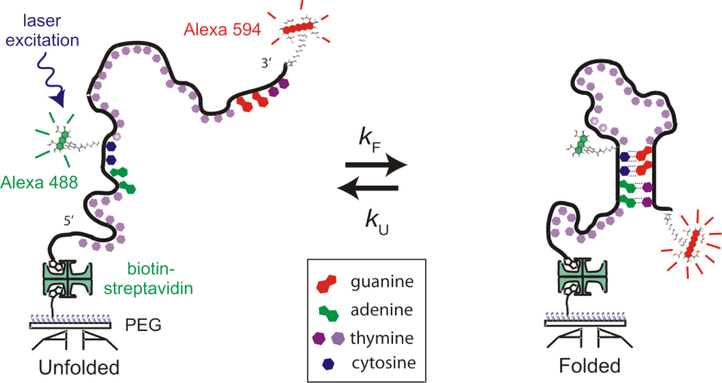
FIG. 2.

Schematic diagram of the single-stranded DNA construct [5’-AACC(T₂₁)GGTT-3’] in an unfolded and a hairpin-folded conformation with fluorescent dye labels and immobilized on a polyethylene glycol coated coverslip via a biotin-streptavidin-biotin linkage. k_F and k_U are the folding and unfolding rate coefficients. The 2 thymines that form base pairs in the folded hairpin are distinguished by a darker shading.

Experimental results.

The ideal comparison would be to study the same DNA hairpins used in the force experiments. However, that is not yet possible because their high stability and low transition frequency make them inaccessible to single molecule FRET measurements, which require folding and unfolding times on the millisecond time scale or less for acquiring data before fluorophore bleaching at the necessarily high illumination intensities terminates the photon trajectories. The DNA hairpin employed in our study has a stem of four base pairs with a flexible loop consisting of 21 thymines (Figure 2). This hairpin was selected because the loop is sufficiently long to result in a significantly lower FRET efficiency in the unfolded compared to the folded state and the several hundred microsecond folding and unfolding times [29, 30] are sufficiently short for the acquisition of many transitions. In addition, analysis of the photon trajectories is much simplified by the fact that this hairpin behaves like a two-state system, i.e. a system with only folded and unfolded populations detectable at equilibrium and at all times in kinetic experiments

Single molecule fluorescence measurements were made using a confocal microscope system (see SI for details). Initial measurements carried out at power densities of ~2 kW/cm² resulted in an average detection rate of 120 photons/ms and produced photon trajectories that were long enough to observe multiple folding and unfolding transitions prior to bleaching of either the donor or acceptor fluorophore. The transition frequency, however, was too high to obtain waiting time distributions for the determination of rate coefficients from FRET efficiency [$E=n_{acceptor}/(n_{acceptor}+n_{donor})$] trajectories. Instead, precise rate coefficients were determined from a photon-by-photon analysis of the trajectories using the maximum likelihood method of Gopich and Szabo [24, 31]. By maximizing a likelihood function, their method yields the parameters of an assumed model that are most consistent with the photon trajectories consisting of colors (donor or acceptor) and intervals between detected photons. The likelihood function for the j^th trajectory consisting of N photons is

$$L_j=1^{\text{T}}\prod _{i=2}^N\left\{F(c_i)\exp \left[K{\tau }_i\right]\right\}F(c_1)p_{eq}$$ (3)

where c_i is the color of the i^th photon in the trajectory, τ_i is the time interval between the i^th and the (i-1)^th photon, F is the photon color matrix where F(acceptor) = E and F(donor) = I – E, E is a diagonal matrix of the FRET efficiencies of the states, I is the identity matrix, K is the rate matrix that depends on the specific model, p_eq is a column vector that gives the equilibrium populations of folded and unfolded states, and 1^T is the row vector (1 1) for a two-state system. This form of the likelihood function is valid if the total (acceptor plus donor) photon count rate is approximately the same in each state, as is the case in our experiments. The two-state rate matrix is $K_{2-\text{state}}=\left(\begin{array}{cc}-k_{\text{U}}& k_{\text{F}}\\ k_{\text{U}}& -k_{\text{F}}\end{array}\right)$. The rate coefficients and FRET efficiencies that resulted from applying equation (3) to 200 photon trajectories with an average length of 60 ms and an average count rate of 120 photons/ms are given in Table SI of the Supplementary Information.

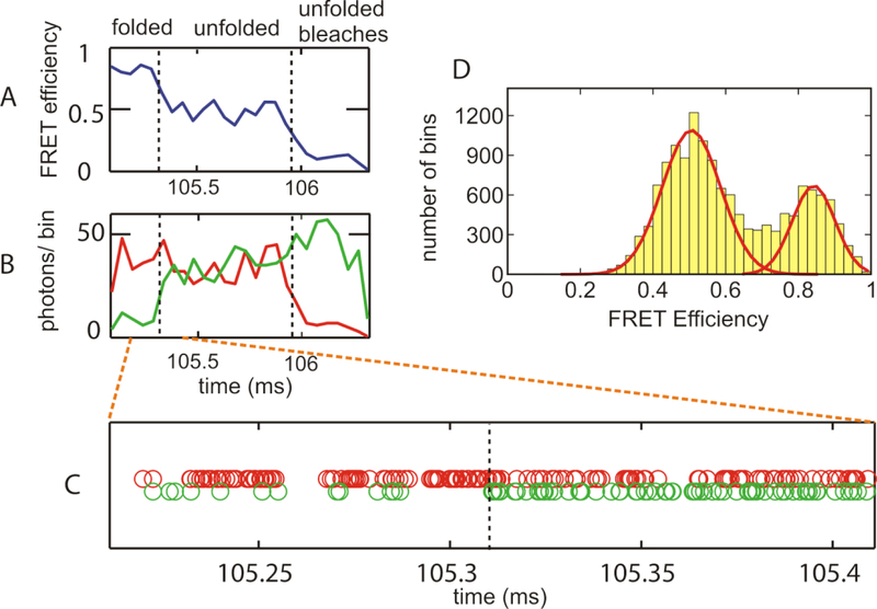
The adequacy of the two-state model was confirmed using several criteria. First, 50 μs binning of the data collected at high illumination intensity shows only 2 peaks, corresponding to folded and unfolded states, with widths accounted for by shot noise (Figure 3D). In addition, the histogram constructed from 1 ms binning at lower intensity (120 photons/ms) used for determining rate coefficients is nearly identical to the histogram constructed by re-coloring the trajectories assuming a two-state model (see SI and Figure S2) [24, 31]. Finally, the decay rate of 3.7 ms⁻¹ for the donor-acceptor cross-correlation function, which is a totally independent analysis of the immobilization data [32], is close to the sum of the rate coefficients of 5.1 ms⁻¹ (Figure S3 and Table S1) from the maximum likelihood, the difference being readily explained by donor blinking [33].

FIG. 3.

Representative single molecule FRET data for immobilized DNA hairpin at high power density (20 kW/cm² and an average count rate of 870 photons/ms). (A) FRET efficiency trajectory. FRET efficiency was calculated for photons collected in 50 μs bins (B) Trajectories of donor (green) and acceptor (red) fluorescence (50 μs bins). (C) Photon trajectory. Each circle represents a detected photon. Red circles (upper row) are acceptor photons. Green circles (lower row) are donor photons. The dashed line indicates a transition predicted by the Viterbi algorithm [34, 35]. (D) FRET efficiency histogram (power density of 20 kW/cm²; 870 detected photons/ms) calculated from photons in 50 μs bins [36]. The continuous red curves are Gaussian fits to the 2 peaks of the histogram using the width expected from shot noise. Intermediate values of the FRET efficiency contribute to the histogram, because ~15% of the bins used to construct the histogram contain a transition between folded and unfolded states.

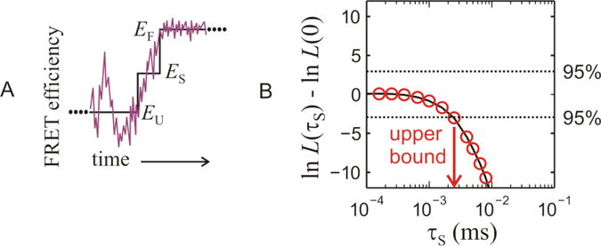
As in previous studies [22, 23], to analyze trajectories at high illumination intensity (Figure 3A, B and C,) for transition path time measurements, we employed a model consisting of the simplest discretization of a transition path, with a single virtual “step” state treated as a kinetic intermediate having a FRET efficiency midway between the folded and unfolded states (Figure 4). The average time spent between the folded and unfolded states during the transition path – the lifetime of this step state (τ_S = 1/2k_S) – is therefore identified as the average transition path time. This simplification allowed us to use a 3-state kinetic model for calculating the value of likelihood function. The rate matrix K of equation (3) now becomes

$$K_{\text{3-state}}=\left(\begin{array}{ccc}-k_{\text{U'}}& k_{\text{S}}& 0\\ k_{\text{U'}}& -2k_{\text{S}}& k_{\text{F'}}\\ 0& k_{\text{S}}& -k_{\text{F'}}\end{array}\right),$$ (4)

where k_U’ and k_F’ are related to parameters known from the low intensity experiments (see details in SI and parameters in Table SI), so only a single parameter, k_S, the rapid rate from the step state to the folded or unfolded state, needs to be varied to maximize the likelihood function. The values of the likelihood function for each trajectory were computed as described in Ref. [22] with unique values of E_F, E_U, and E_S for each trajectory, since the local environment of each molecule immobilized on the glass slightly affects its FRET efficiency. The total log-likelihood for a data set of n transitions is given by $\ln L=\sum _{m=1}^n\ln L_m$. The likelihood function for the m^th segment containing a single transition is given by equation (3), but with p_eq replaced by v_initial and 1^T replaced by v_final, since the initial and final states are known.

FIG. 4.

Kinetic model and maximum likelihood analysis of photon trajectories. (A) The noisy curve is a schematic of the instantaneous FRET for a transition path from the unfolded to folded states. The step curve is the simplest discretization of the path with average FRET efficiencies E_U for the unfolded state, E_F for the folded state, and an intermediate value E_S = (E_U + E_F)/2 for the virtual step state, (B) Comparison of the values of the likelihood function from the three state analysis, L(τ_S), and a two-state analysis with an instantaneous transition, L(0), calculated for 780 transitions from immobilized molecules. The result of the calculation is that no lifetime greater than 2.5 μs is detected by the measurement, so the average transition path time is shorter than 2.5 μs. Acceptor blinking can interfere with the transition path time analysis [33], but was effectively eliminated by not including transitions in which there are nearby strings of 8 or more donor photons (See the Supplementary Information for details).

Figure 4B shows the difference in the values of the log-likelihood functions, $\Delta \ln L=\ln L({\tau }_S)-\ln L(0)$, where the likelihood function, L, is for the three state model as described above for 780 transitions between folded and unfolded states. L(0) represents the case for an instantaneous transition between the folded and unfolded states in a two-state model. Thus, the plot shows whether a three-state model with a finite transition path time or a two-state model with an instantaneous transition is more likely by comparing the values of the likelihood function for each model. The dashed horizontal lines correspond to the 95% confidence levels defined by $L({\tau }_S)/[L({\tau }_S)+L(0)]=0.95\text{\hspace{0.17em}\hspace{0.17em}or\hspace{0.17em}\hspace{0.17em}}L(0)/[L({\tau }_S)+L(0)]=0.95$. For a given value of τ_S, ΔlnL = 0 indicates that both models are equally consistent with the data, while values of ΔlnL > 0 indicate that the 3-state model is more likely and the value of τ_S at a peak in ΔlnL > 3 corresponds to the average transition path time [22, 23]. When no peak is observed, the value of τ_S at ΔlnL = - 3 indicates with 95% confidence that an instantaneous model is more consistent with the data and that there is no lifetime detected in the trajectories larger than this value [22]. For our data ΔlnL = - 3 when τ_S = 2.5 μs, which is therefore an upper bound for the average transition path time. Re-coloring the same set of trajectories for several fixed values of τ_S demonstrates that for the number of observed transitions, photon count rate and FRET efficiencies in our experiments no significant peaks could possibly be observed for t_TP ≲ 5 μs.

Discussion.

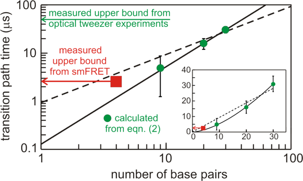
Our determination of 2.5 μs for the upper bound for the average transition path time of this DNA hairpin represents a major improvement in time resolution compared with the 50 μs upper bound that could be obtained in the force spectroscopic experiments [17]. A comparison of our experimental result with the predictions from the optical tweezer experiments based on equation (2) (Figure 5) raise interesting and important issues. To explain the predicted dependence of the average transition path time (t_TP) on the number of base pairs in the stem (N) (Figure 5) Woodside and coworkers made the assumption that t_TP ~ N [17]. On the other hand, Frederickx et al. developed a theoretical model for the transition path time at zero force, confirmed by coarse-grained simulations, that yielded a power law, t_TP ~ N^α, with α = 1 + ν, where ν = 0.59 is the Flory exponent [28]. Their theoretical curve with a best-fit α of 1.6 ± 0.4 corresponds remarkably well with the experimental data (Figure 5). The non-linear dependence in their theory results from a diffusion coefficient that is position dependent because of an increase in strand tension as the stem zips up.

FIG. 5.

Transition path time as a function of the number of base pairs in the stem of the folded structure. The green circles with error bars were calculated from equation (2) by Neupane et al. [17] from force spectroscopic determinations of ΔG*, D*, and k_b for DNA hairpins with stem lengths of 20 and 30 base pairs and a DNA aptamer with a stem of 9 base pairs. The red square with an arrow attached is the upper bound of 2.5 μs determined in this work for the 4-base-pair stem of the DNA hairpin using single molecule FRET. The broken curve is from Neupane et al., which assumes that t_TP ~ N, while the continuous curve is t_TP ~ N^α with α = 1.6 from Frederickx et al. [28]. Insert is same points and curves on a linear scale.

Comparison between our measured upper bound for the transition path time and the predicted value from the parameters determined in Woodside’s force measurements has several caveats, including the fact that the polythymine loop in the fluorescence measurements is much larger (21 compared to 4) and the important assumptions that both the experimentally-determined diffusion coefficient and barrier-top curvature used by Woodside and coworkers in calculating the transition path times from equation (2) are unchanged when the force is removed. Nevertheless, the close correspondence of our upper bound of 2.5 μs, compared to the predicted values of 3.6 μs and 1 μs from the linear and power law fits to the force data, respectively, is a significant result, for it is one of the most convincing pieces of experimental evidence that the diffusion on a 1D free energy surface scenario may indeed provide a quantitative description of a complex self-assembly process. Another important test of the 1D scenario is currently being carried out by analyzing the all-atom molecular dynamics simulations of protein folding by the D.E. Shaw group. Comparisons of mean first passage and transition path times with those calculated from the 1D free energy surface and diffusion coefficient from the simulations using the number of native contacts as the reaction coordinate are so far in good agreement (Chung, Piana, Shaw, and Eaton, unpublished results; Zheng and Best, unpublished results). If both experiments and atomistic simulations show that the theory for motion of a single Brownian particle on a 1D surface does turn out to be near quantitatively perfect for folding DNA hairpins and proteins, it raises the interesting and important question of why such a simple theory works so well.

References:

- [1].Kramers HA, Brownian motion in a field of force and the diffusion model of chemical reactions. Physica VII, 284 (1940). [Google Scholar]
- [2].Bryngelson JD, and Wolynes PG, Intermediates and barrier crossing in a random energy-model (with applications to protein folding). J. Phys. Chem 93, 6902 (1989). [Google Scholar]
- [3].Dobson CM, Sali A, and Karplus M, Protein folding: A perspective from theory and experiment. Angew. Chem 37, 868 (1998). [DOI] [PubMed] [Google Scholar]
- [4].Wolynes PG, Recent successes of the energy landscape theory of protein folding and function. Quart. Rev. Biophys 38, 405 (2005). [DOI] [PubMed] [Google Scholar]
- [5].Faccioli P, Sega M, Pederiva F, and Orland H, Dominant pathways in protein folding. Phys. Rev. Lett 97, 108101 (2006). [DOI] [PubMed] [Google Scholar]
- [6].Best RB, and Hummer G, Diffusive model of protein folding dynamics with Kramers turnover in rate. Phys. Rev. Lett 96, 228104 (2006). [DOI] [PubMed] [Google Scholar]
- [7].Shakhnovich E, Protein folding thermodynamics and dynamics: Where physics, chemistry, and biology meet. Chem. Rev 106, 1559 (2006). [DOI] [PMC free article] [PubMed] [Google Scholar]
- [8].Munoz V, Conformational dynamics and ensembles in protein folding. Annu. Rev. Biophys. Biomol. Struct 36, 395 (2007). [DOI] [PubMed] [Google Scholar]
- [9].Thirumalai D, O’Brien EP, Morrison G, and Hyeon C, Theoretical perspectives on protein folding. Annu. Rev. Biophys 39, 159 (2010). [DOI] [PubMed] [Google Scholar]
- [10].Best RB, and Hummer G, Coordinate-dependent diffusion in protein folding. Proc. Natl. Acad. Sci. USA 107, 1088 (2010). [DOI] [PMC free article] [PubMed] [Google Scholar]
- [11].Chan HS, Zhang Z, Wallin S, and Liu Z, Cooperativity, local-nonlocal coupling, and nonnative interactions: principles of protein folding from coarse-grained models. Ann. Rev. Phys. Chem 62, 301 (2011). [DOI] [PubMed] [Google Scholar]
- [12].Whitford PC, Sanbonmatsu KY, and Onuchic JN, Biomolecular dynamics: order-disorder transitions and energy landscapes. Reports Prog. Physics 75, 076601 (2012). [DOI] [PMC free article] [PubMed] [Google Scholar]
- [13].Henry ER, Best RB, and Eaton WA, Comparing a simple theoretical model for protein folding with all-atom molecular dynamics simulations. Proc. Natl. Acad. Sci. USA 110, 17880 (2013). [DOI] [PMC free article] [PubMed] [Google Scholar]
- [14].Best RB, Hummer G, and Eaton WA, Native contacts determine protein folding mechanisms in atomistic simulations. Proc. Natl. Acad. Sci. USA 110, 17874 (2013). [DOI] [PMC free article] [PubMed] [Google Scholar]
- [15].Gelman H, and Gruebele M, Fast protein folding kinetics. Quart. Rev. Biophys 47, 95 (2014). [DOI] [PMC free article] [PubMed] [Google Scholar]
- [16].Woodside MT, Anthony PC, Behnke-Parks WM, Larizadeh K, Herschlag D, and Block SM, Direct measurement of the full sequence-dependent landscape of a nucleic acid. Science 314, 1001 (2006). [DOI] [PMC free article] [PubMed] [Google Scholar]
- [17].Neupane K, Ritchie DB, Yu H, Foster DAN, Wang F, and Woodside MT, Transition path times for nucleic acid folding determined from energy-landscape analysis of single-molecule trajectories. Phys. Rev. Lett 109, 068102 (2012). [DOI] [PubMed] [Google Scholar]
- [18].Hinczewski M, Gebhardt JCM, Rief M, and Thirumalai D, From mechanical folding trajectories to intrinsic energy landscapes of biopolymers. Proc. Natl. Acad. Scie. USA 110, 4500 (2013). [DOI] [PMC free article] [PubMed] [Google Scholar]
- [19].Woodside MT, and Block SM, Reconstructing folding energy landscapes by single-molecule force spectroscopy. Ann. Rev. Biophys 43, 19 (2014). [DOI] [PMC free article] [PubMed] [Google Scholar]
- [20].Woodside MT, Lambert J, and Beach KSD, Determining intrachain diffusion coefficients for biopolymer dynamics from single-molecule force spectroscopy measurements. Biophys. J 107, 1647 (2014). [DOI] [PMC free article] [PubMed] [Google Scholar]
- [21].Engel MC, Ritchie DB, Foster DAN, Beach KSD, and Woodside KT, Reconstructing folding energy landcsape profiles from nonequilibrium pulling curves with an inverse Weierstrass integral transform. Phys. Rev. Lett 113, 238104 (2014). [DOI] [PubMed] [Google Scholar]
- [22].Chung HS, McHale K, Louis JM, and Eaton WA, Single-molecule fluorescence experiments determine protein folding transition path times. Science 335, 981 (2012). [DOI] [PMC free article] [PubMed] [Google Scholar]
- [23].Chung HS, and Eaton WA, Single-molecule fluorescence probes dynamics of barrier crossing. Nature 502, 685 (2013). [DOI] [PMC free article] [PubMed] [Google Scholar]
- [24].Chung HS, and Gopich IV, Fast single-molecule FRET spectroscopy: theory and experiment. Phys. Chem. Chem. Phys 16 18644 (2014). [DOI] [PMC free article] [PubMed] [Google Scholar]
- [25].Chung HS, Louis JM, and Eaton WA, Experimental determination of upper bound for transition path times in protein folding from single-molecule photon-by-photon trajectories. Proc. Natl. Acad. Sci. USA 106, 11837 (2009). [DOI] [PMC free article] [PubMed] [Google Scholar]
- [26].Chaudhury S, and Makarov DE, A harmonic transition state approximation for the duration of reactive events in complex molecular rearrangements. J. Che, Phys 133 (2010). [DOI] [PubMed] [Google Scholar]
- [27].Hummer G, and Eaton WA, Viewpoint: Transition path times for DNA and RNA folding from force spectroscopy. Physics, 5, 87 (2012). [Google Scholar]
- [28].Frederickx R, in’t Veld T, and Carlon E, Anomalous dynamics of DNA hairpin folding. Phys. Rev. Lett 112, 198102 (2014). [DOI] [PubMed] [Google Scholar]
- [29].Jung J, Ihly R, Scott E, Yu M, and Van Orden A, Probing the complete folding trajectory of a DNA hairpin using dual beam fluorescence fluctuation spectroscopy. J. Phys. Chem. B 112, 127 (2008). [DOI] [PubMed] [Google Scholar]
- [30].Narayanan R, Zhu L, Velmurugu Y, Roca J, Kuznetsov SV, Prehna G, Lapidus LJ, and Ansari A, Exploring the energy landscape of nucleic acid hairpins using laser temperature-jump and microfluidic mixing. J. Am. Chem. Soc 134, 18952 (2012). [DOI] [PubMed] [Google Scholar]
- [31].Gopich IV, and Szabo A, Decoding the pattern of photon colors in single-molecule FRET. J. Phys. Chem. B 113, 10965 (2009). [DOI] [PMC free article] [PubMed] [Google Scholar]
- [32].Chung HS, Gopich IV, McHale K, Cellmer T, Louis JM, and Eaton WA, Extracting rate coefficients from single-molecule photon trajectories and FRET efficiency histograms for a fast-folding protein. J. Phys. Chem. A 115, 3642 (2011). [DOI] [PMC free article] [PubMed] [Google Scholar]
- [33].Chung HS, C. T, L. JM, and Eaton WA, Measuring ultrafast protein folding rates from photon-by-photon analysis of single molecule fluorescence trajectories. Chem. Phys 422, 229 (2013). [DOI] [PMC free article] [PubMed] [Google Scholar]
- [34].Rabiner LR, A tutorial on hidden Markov models and selected applications in speech. Proc. IEEE 77, 257 (1989). [Google Scholar]
- [35].Viterbi AJ, Error bounds for convolution codes and an asymptotically optimum decoding algorithm. IEEE Trans. Information Theory 13, 260 (1967). [Google Scholar]
- [36].Gopich IV, and Szabo A, Theory of single-molecule FRET efficiency histograms. Adv. Chem. Phys 146, 245 (2012). [Google Scholar]
Associated Data
This section collects any data citations, data availability statements, or supplementary materials included in this article.