Abstract
Purpose
To develop a novel framework for rapid, intrinsic head motion measurement in MRI using FID navigators (FIDnavs) from a multi-channel head coil array.
Methods
FIDnavs encode substantial rigid-body motion information; however, current implementations require patient-specific training with external tracking data to extract quantitative positional changes. In this work, a forward model of FIDnav signals was calibrated using simulated movement of a reference image within a model of the spatial coil sensitivities. An FIDnav module was inserted into a non-selective 3D FLASH sequence and rigid-body motion parameters were retrospectively estimated every readout time using non-linear optimization to solve the inverse problem posed by the measured FIDnavs. This approach was tested in simulated data and in seven volunteers, scanned at 3T with a 32-channel head coil array, performing a series of directed motion paradigms.
Results
FIDnav motion estimates achieved mean absolute errors of 0.34 ± 0.49 mm and 0.52 ± 0.61° across all subjects and scans, relative to ground-truth motion measurements provided by an electromagnetic tracking system. Retrospective correction with FIDnav motion estimates resulted in substantial improvements in quantitative image quality metrics across all scans with intentional head motion.
Conclusions
Quantitative rigid-body motion information can be effectively estimated using the proposed FIDnav-based approach, which represents a practical method for retrospective motion compensation in less cooperative patient populations.
Keywords: MRI motion measurement, motion correction, FID navigators, coil sensitivity profile
INTRODUCTION
MRI is highly sensitive to motion and resulting artifacts can significantly degrade image quality. Motion is particularly problematic for clinical imaging of pediatric or other uncooperative patient populations, in many cases leading to non-diagnostic images requiring a repeat scan. A variety of motion prevention strategies have been adopted including physical restraints, training and sleep manipulation in infants, which are partially effective, but not always practical (1). Sedation and general anesthesia are commonly used when imaging children (2); however, these are expensive and time-consuming to administer and there are increasing concerns over their potential long-term adverse side effects (3). Technological developments over the last few decades, from fast acquisition schemes (4,5) and parallel imaging (6–8), to advanced methods such as simultaneous multi-slice acquisitions (9) and compressed sensing (10), have enabled a reduction in imaging times, and hence inherent sensitivity to motion. However, despite these advances, scan times in routine brain MRI protocols still reach the order of several minutes, highlighting the need for techniques that can explicitly measure and correct for subject motion.
Various methods have been proposed to compensate for motion (11) either retrospectively, by modifying the acquired k-space data during reconstruction, prospectively, via real-time update of the image acquisition (12) or a combination (13). To correct for motion, subject movement must first be estimated, either using an external tracking system or from the MR data itself. Measurement noise (precision) should be a fraction of the target pixel resolution to avoid introducing additional artifacts (14). Optical (13,15) or electromagnetic (16,17) sensors may be used to measure motion with high temporal resolution and reported accuracy on the order of ±0.1 mm/°. However, these require integration of MR compatible hardware and fixation of a fiducial marker on the subject, which may compromise clinical workflow and will be sensitive to any non-rigid or skin motion. Optical trackers additionally require careful cross-calibration and a line of sight between the camera system and optical sensor, which may be difficult to achieve. In practice, MR-based motion tracking methods are arguably more convenient, particularly for imaging non-compliant patients. Motion-robust k-space trajectories, including radial (18), spiral (19) and periodically rotated overlapping parallel lines with enhanced reconstruction (PROPELLER) (20), help alleviate motion artifacts by oversampling the center of k-space and may be used for self-navigation prior to the final image reconstruction (20–22). Drawbacks of these approaches include reduced acquisition efficiency, increased reconstruction complexity, and most are limited to in-plane motion correction. Navigator methods acquire additional data to determine positional information relative to a reference signal. Navigators may be based in image space e.g. PROMO (23), fat navigators (24) and volumetric navigators (vNavs) (25), or k-space e.g. spherical (26), orbital (27) and cloverleaf (28) navigator echoes. There is usually a trade-off between tracking accuracy and the navigator acquisition time, meaning most navigator acquisitions are limited to sequences containing sufficient dead time.
Free induction decay (FID) navigation, originally developed to correct for system instability and physiological fluctuations in functional MRI (29), exploits the fact that individual coils are spatially sensitive to local signal changes from different regions of the head to detect motion within the coil array (30). FID navigators (FIDnavs) sample the k-space center without any imaging gradients and are an attractive option for monitoring motion as they have negligible impact on the magnetization or overall scan time. This enables motion detection with a high temporal resolution, which may be used to trigger a prospective motion correction strategy with selection of an appropriate threshold (31). The ability of FIDnavs to recognize previously determined head positions within the magnet has also been demonstrated (32); however, this approach currently entails a patient-specific training session prior to imaging, requiring the subject to perform a series of choreographed head movements with external ground-truth motion measurements, in order to train a pattern recognition algorithm. This is impractical in many clinical scenarios and represents a significant barrier to widespread clinical implementation of this approach.
The purpose of this work is to develop a novel framework for motion measurement using FIDnavs from multi-channel head coil arrays, without the need for choreographed training or additional ground-truth motion data. We propose calibrating FIDnav signal changes using simulation of the acquisition physics and the effect of head motion upon the FIDnav measurements from each coil. This approach relies on construction of an appropriate forward model to predict FIDnav signal changes due to head motion. Here, we validate this approach in simulations and demonstrate the accuracy of derived motion measurements and the efficacy of retrospective artifact correction in a series of directed motion experiments in volunteers.
THEORY
FID Navigation
Multi-channel coil arrays are routinely used in clinical brain MRI examinations and prototype head coil designs with up to 64 array elements are now becoming commercially available (33). According to the Principle of Reciprocity (34), the strength of the received MR signal in an individual coil element is proportional to the ratio of the magnetic field B1 generated by the coil to the coil current I, per the Biot-Savart Law (35):
| [1] |
where ds is a differential element of wire along the coil path, ( ) is the displacement vector from the wire element ds to the point within the object where the magnetic field is computed and is the magnetic permeability constant. FIDnavs measure the MR signal without any spatial encoding and may be represented as:
| [2] |
where is the complex FIDnav from the jth coil, is the effective proton density of the original image and is the complex coil sensitivity profile (CSP) at position . The received signal is dependent on the distance between the object and the coil element; therefore, movement of the object within the coil array results in changes in the measured FIDnav. We propose that a forward model of the magnitude of the FIDnavs may be constructed to estimate rigid-body motion parameters describing the head position within the magnet:
| [3] |
where is a real-valued model matrix describing how the spatial sensitivity map of each coil and the spin density of the object being imaged result in FIDnav measurements and is a vector whose elements are the six rigid-body motion parameters describing the change in the object’s position and orientation at time t. If a linear relationship between FIDnav signal changes and rigid-body motion is assumed, , C is an Nc 7 matrix (where Nc is the number of channels) and motion parameters can be computed from the inverse of Equation 3. Given the non-linear nature of the coil sensitivities (Eq. 1), we propose that a higher-order polynomial regression model may provide a closer approximation to Equation 1 and more effectively characterize larger amplitude motion within the coil array. For a second-order polynomial regression model, (i.e. a 28 1 vector parameterized by six unknowns), C is an Nc 28 matrix and Equation 3 may then be solved for xt in a least-squares sense using a suitable non-linear optimization algorithm. A schematic of the proposed FIDnav motion measurement approach is shown in Figure 1.
FIG. 1.
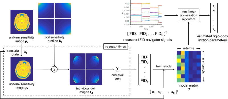
Proposed FID navigator motion measurement system.
Coil Sensitivity Estimation and Extrapolation
This approach assumes that the CSPs are static and independent of the head position and orientation, which should be valid for small head movements (36). It also requires that CSPs can be accurately estimated over the full range of possible head positions within the field of view (FOV). One solution is to explicitly calculate the CSPs via the Biot-Savart Law (37); however, this is challenging as it requires a priori knowledge of the exact coil positions and may also be affected by unpredictable coil loading and coupling between array elements. In practice, CSPs are typically derived from low-resolution complex surface coil images normalized by either a root-sum-of-squares image or a body coil image, which is assumed to have a spatially uniform sensitivity (7). This approach necessitates extrapolation of the measured CSP beyond the boundaries of the initial object position, which may be achieved by fitting a parametric surface in the form of local polynomials (7) or global basis functions (splines) (38). In this work, CSPs were extrapolated across the imaging FOV by fitting a series of 3D radial basis functions (RBFs), described in the Appendix.
METHODS
Numerical Simulations
To validate the proposed approach, numerical simulations were performed in Matlab (R2016b; Mathworks, Natick, MA). 3D CSPs were simulated for 16 channels by numerically integrating Equation 1 along each coil path to obtain an approximation of the B1 field (39). Simulation parameters were as follows: FOV = 300 mm, coil radius = 45 mm, distance of coil from image center = 150 mm. A 2-mm isotropic proton density-weighted axial brain volume (40) was used as the test object. Individual coil images were simulated by point-wise multiplication of the test object with the CSPs and the FIDnav signal was computed as the complex sum of each coil image. FIDnavs were calculated for series of 500 rigid-body motions in six degrees of freedom (DOF) with maximum vector norms of 10 mm/° to generate a training dataset. Resampling was implemented in C++ using the Insight Toolkit (ITK), using Kaiser-Bessel window (sinc) interpolation to preserve information at the edges of the image. Simulated FIDnavs were used to calibrate first and second-order polynomial regression models to compute the model matrices C.
The accuracy (mean absolute error) and precision (standard deviation of the error) of FIDnav motion tracking was tested for a series of 500 compound rigid-body movements (6 DOF) with increasing displacement and rotation amplitudes. Multi-variate complex Gaussian noise with zero-mean, standard deviation (where is the mean of the jth FIDnav signal and SNR = 400 is the signal-to-noise ratio of the FIDnav time course) and covariance matrix ( = 1; 0 < < 0.25) was added to the simulated FIDnavs. An efficient numerical non-linear optimization algorithm BOBYQA (41) was then used to compute motion parameters xt from the magnitude of the noisy FIDnav signal vector yt by solving the following minimization problem:
| [4] |
where kt is a scaling factor introduced to account for bulk magnitude fluctuations in the FIDnav signal over time. This was seeded with motion estimates from the linear model, computed from the inverse of Equation 3. To determine the minimum resolution requirements for the reference image, the simulation was repeated using successively lower resolution images for the training dataset. Simulation of simple 1D 10 mm/° translations and rotations was also performed to further explore the nature of the errors for each of the regression models in the presence of large amplitude motion.
MRI Experiments
Data Acquisition
Seven volunteers were scanned at 3T (Siemens Healthcare, Erlangen, Germany) using a 32-channel head coil. Volunteers gave written informed consent prior to imaging and all scans were performed in accordance with the local Institutional Review Board protocol. Two reference images were acquired with the surface and body coils, respectively, using a sagittal, non-selective 3D fat-suppressed fast low-angle shot (FLASH) sequence for estimation of the CSPs, effective proton distribution and noise covariance matrix (Fig. 2a). Acquisition parameters were as follows: repetition time (TR) = 22 ms, echo time (TE) = 1 ms, flip angle ( ) = 20°, receiver bandwidth (RBW) = 87.5 kHz, FOV = 256 256 224 mm, 4 mm isotropic resolution, total acquisition time (TA) = 1 min 23 s.
FIG. 2.
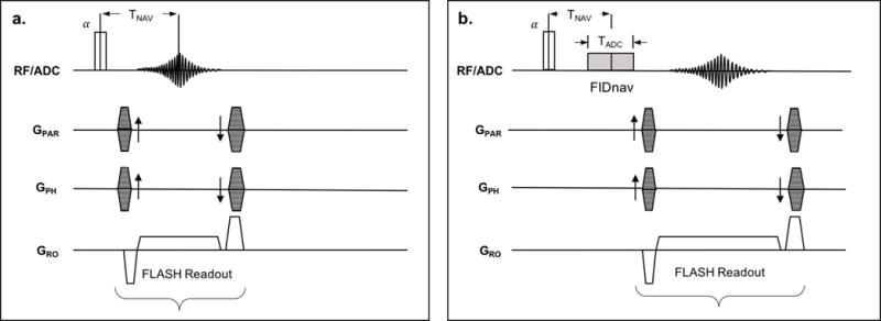
Reference 3D FLASH (a) and FID-navigated 3D FLASH (b) pulse sequences. The echo time of the reference image is designed to match center of the FIDnav (TNAV).
An FIDnav module was inserted into a 3D FLASH sequence immediately after the non-selective excitation pulse and before the imaging readout (Fig. 2b). Following excitation, 320 complex FID data points were sampled during an analog-to-digital converter (ADC) readout, with an acquisition time (TADC) of 2 ms. TADC was chosen so that the navigator time (TNAV; defined as the center of the FIDnav readout) was equal to the TE of the reference image, so that the simulated FIDnav signal (Eq. 2) should match the measured FIDnav. As the FIDnav utilizes the same excitation pulse as the host sequence, this increases the minimal TE and TR of the sequence by TADC (2 ms). Fat suppression was applied to prevent dephasing of the FIDnav signal over the sampling time due to the different resonant frequencies of water and fat.
A total of five FID-navigated fat-suppressed T1-weighted anatomical scans were then acquired with the following acquisition parameters: TADC/TNAV = 2/1 ms, TR/TE = 22/3.96 ms, = 20°, RBW = 87.5 kHz, FOV = 256 256 224 mm, 1.3 1.3 2 mm resolution, TA = 8 min 15 s. Subjects were instructed to perform the following directed motion experiments to simulate a variety of motion conditions:
Remain as still as possible for the duration of the scan (small involuntary motion only)
Perform a smooth head nodding motion, beginning 30 seconds into the scan and continuing for the duration of the scan
Perform a smooth head shaking motion, as above
Perform a series of eight abrupt head jerks (resulting in a repositioning of the head within the magnet), spaced approximately 1 minute apart
Perform a continuous, free motion during the central two minutes of the scan, remain still for the remainder of the scan
All instructions were given verbally through the scanner intercom system. An electromagnetic (EM) tracking system (Robin Medical Inc., Baltimore, MD) was used to provide ground-truth motion data. Four sensors were affixed to a flexible strip, which was tightly attached to a headband worn by the subject and the relative position and orientation of each sensor was measured every TR.
Data Analysis
Complex k-space data from each channel were reconstructed in Matlab. The noise covariance was estimated from a small region of background voxels in the reconstructed surface coil images. CSPs were estimated by taking the ratio of the complex surface and body coil images. A mask was defined to segment the background region by applying an empirical thresholding criteria to the body coil image, which was the same for all volunteers. A sparse set of reliable data points were selected from the measured CSPs in the foreground region using a local first-order polynomial fitting criteria (42). Specifically, a linear plane was fit to local regions centered on each pixel within the bias field map (computed by taking the sum-of-squares of the ratio data) and the sum-of-square difference was computed between the measured data and each fitted linear plane. Points with errors <1% were included as nodes for the RBF extrapolation. A linear RBF (biharmonic spline) was fit to this sparse set of data points to extrapolate the CSP information, as described in the Appendix. The regularization parameter was empirically chosen to be equal to one voxel width (4 mm) to obtain a smooth approximation of the CSP information across the whole FOV (Supporting Information Fig. S1).
The reference image was created using Roemer optimal reconstruction of the individual coil images, as this exploits the higher SNR of the multi-channel surface coils, whilst retaining the uniform sensitivity of the body coil (35). As the acquisition was non-selective, the reference image was partitioned into two locally rigid regions: the head (assumed to move as a rigid body) and the neck-and-shoulder region (assumed to remain stationary). Binary masks were prospectively defined for each subject by positioning a single oblique plane on the reference image. Masks were convolved with a Gaussian kernel to enforce a smooth transition between the moving and stationary spin densities. The simulated FIDnav signal was obtained by summing over both spatial regions (see Supporting Information Fig. S2), assuming these are approximately separable, subject to some small errors as a result of localized gaps and overlaps near the boundaries of the mask (43). The masked reference image was rotated and translated (6 DOF; maximum amplitude 5 mm/°) and resampled 500 times within this model of the coil array to generate a simulated FIDnav dataset to calibrate a second-order polynomial regression model (Fig. 1). 50 complex FIDnav readout samples (centered around TNAV) were averaged prior to magnitude extraction, generating a single measurement for each coil and time point. The resulting FIDnav time course was low-pass filtered, using a Kaiser-Bessel filter with a cut-off frequency of 0.2 Hz, to mitigate the effect of physiological noise (cardiac pulsation and respiration) prior to motion estimation. Measurements from the first five seconds of each dynamic phase were discarded to allow the signal to reach a steady state. Rigid-body motion parameters were then estimated from the measured FIDnavs using non-linear optimization (Eq. 4).
Optimal rigid-body motion parameters were estimated from the position and orientation of the four EM sensors using singular value decomposition (44). Accuracy and precision of FIDnav motion estimates were computed as the mean absolute error and standard deviation of the error, respectively, relative to the ground-truth EM tracking data. The mean voxel displacement (MVD), which describes the mean distance traversed by each voxel within a model of the head (45), was calculated for each subject and motion paradigm as follows:
| [5] |
where is a set of Nv points within a brain region mask, segmented using FSL BET2, (Analysis Group, FMRIB, Oxford, UK) at time t, computed using the EM tracker rotation and displacement estimates relative to the initial position ( ) and Nt is the total number of time points. The residual MVD following retrospective correction with FIDnav motion predictions was also calculated.
Motion estimates from each scan were applied to the raw k-space data to evaluate FIDnav-based retrospective motion correction. Translational and rotational motion correspond to a linear phase shift and rotation of k-space lines, respectively. Reconstruction was performed by regridding the rotated k-space data from each coil (46), as proposed by Gallichan et al. (24). Retrospectively corrected and uncorrected images were registered to the (uncorrected) image volume acquired without any voluntary motion and the voxel-wise normalized root-mean-square error (NRMSE) and the structural similarity (SSIM) index (47) were calculated within the segmented brain region relative to this motion-free reference image. Paired Wilcoxon signed-rank tests were performed to determine if the improvement in these quantitative image metrics following retrospective correction with EM tracking and FIDnav motion estimates were significant.
RESULTS
Model validation
The accuracy and precision of translational and rotational motion estimates for simulated head movements with increasing maximum motion amplitude are displayed in Figure 3a for the linear and non-linear regression models. The linear model exhibits a reduction in accuracy and precision with increasing motion amplitude, whilst the non-linear model retains accuracy and precision on the order of 0.16 ± 0.12 mm and 0.52 ± 0.38° for amplitudes up to 10 mm/°. The 1D simulations reveal that the poor performance of the linear model at larger motion amplitudes is due to “cross-talk” errors, where a change in one motion parameter induces a false change in another (Supporting Information Fig. S3). Figure 3b demonstrates that reducing the resolution of the reference image beyond 5 mm decreases the accuracy and precision of the resulting motion estimates.
FIG. 3.
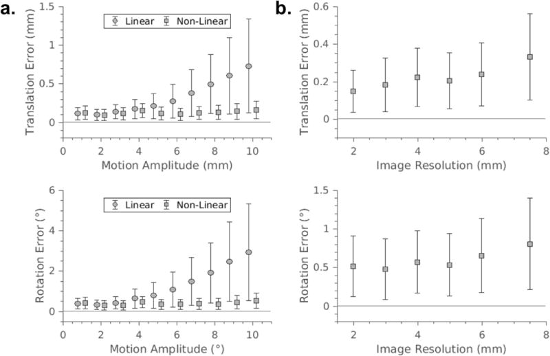
Accuracy and precision of translational and rotational estimates from linear (circles) and non-linear (squares) regression models (a), calculated for trials of 500 simulated data points with increasing motion amplitudes. The non-linear model retains high accuracy and precision with increasing motion amplitudes. Impact of the pixel resolution of the reference image for calibration of the non-linear regression model on the accuracy and precision of FIDnav navigator translational and rotational motion estimates (b), calculated for maximum motion amplitudes of 10 mm/°. There is a trade-off between resolution of the reference image and navigator accuracy.
Accuracy of Head Motion Measurement
Representative FIDnav time courses from each motion paradigm are displayed in Supporting Information Figure S4. Per-TR motion parameters were estimated in ~10 ms using the BOBYQA algorithm to solve the optimization problem posed by the measured FIDnavs. The estimated motion trajectories from the FIDnavs and the EM tracking system from a representative scan with no voluntary motion are shown in Figure 4. Translational motion estimates are in excellent agreement, with both the EM tracker and FIDnavs measuring a slow drift in z-translation over the course of the eight-minute scan. A small bias can be seen in the FIDnav in-plane rotational motion estimates. Several swallowing events can also be observed in the EM tracking data, denoted by the arrows, which introduce small errors into the FIDnav motion estimation at these time points, due to violation of the assumption of rigid-body motion. Similar slow, drift-like motion patterns were observed across all volunteer scans with no intentional motion (n=7) with maximum motion amplitudes on the order of 0.46/0.24/0.61 mm and 0.73/0.82/0.34° for x/y/z translation and rotation. Under these conditions, FIDnavs demonstrated absolute errors on the order of 0.11 ± 0.05/0.08 ± 0.04/0.17 ± 0.08 mm and 0.3 ± 0.17/0.27 ± 0.14/0.36 ± 0.19°.
FIG. 4.
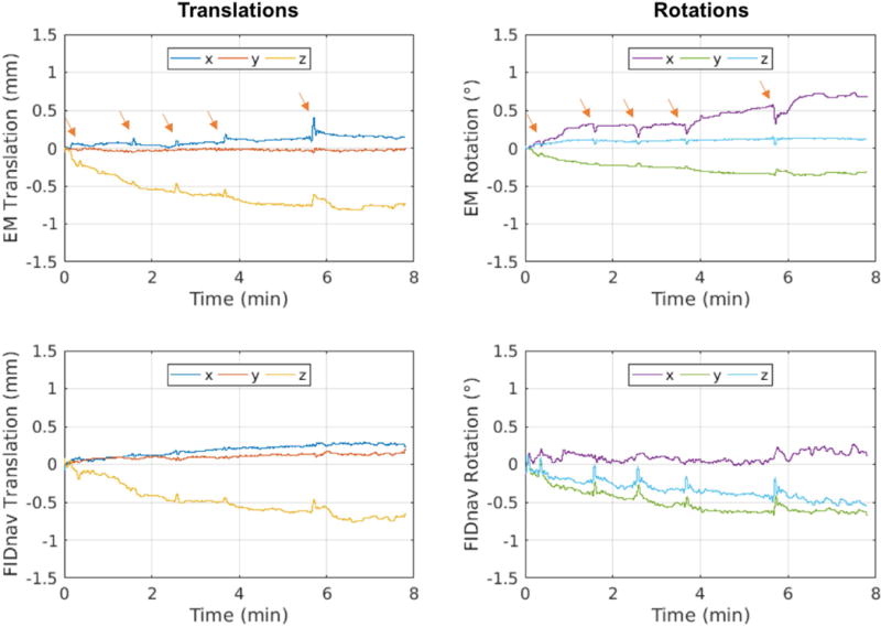
Translational and rotational motion trajectories recorded from the EM tracking system during a volunteer scan (Subject 5) with no intentional motion and corresponding FIDnav motion estimates; arrows denote swallowing events. FIDnav translational measures are in excellent agreement with EM tracking, whilst an additional drift is observed in the FIDnav tracking estimates for in-plane rotation. Swallowing events introduce small errors in FIDnav motion estimation due to the assumption of rigid-body motion.
Figure 5 shows the translational and rotational motion trajectories measured by the EM tracking system and proposed FIDnav measurement system for a subject performing slow continuous head nodding and shaking motion for the duration of the scan. There is good agreement between rigid-body motion estimates from FIDnavs and EM tracking, with FIDnavs tending to slightly underestimate larger amplitude motions. Across all subjects and motion paradigms, FIDnavs demonstrated absolute errors of 0.44 ± 0.68/0.25 ± 0.40/0.31 ± 0.40 mm and 0.67 ± 0.73/0.45 ± 0.57/0.44 ± 0.54° for maximum x/y/z translation and rotation amplitudes on the order of 6.90/3.14/2.57 mm and 13.07/5.15/11.80°. Figure 6 shows the distribution of the translational and rotational errors in each direction for all volunteers and motion paradigms. Larger errors are evident for some scans and motion paradigms (notably for Subject 3 performing the abrupt motion paradigm where the magnitude of x-translation was underestimated), which indicates the limitations of the method for reliably measuring large (>10 mm/°) motion amplitudes. Histograms of the absolute translational and rotational errors for each motion paradigm are shown in Supporting Information Figure S5, alongside the maximum amplitude motion measured in each direction. Across all scans, 94.9% of translational and 85.8% of rotational motion estimates were estimated with errors <1 mm/°.
FIG. 5.
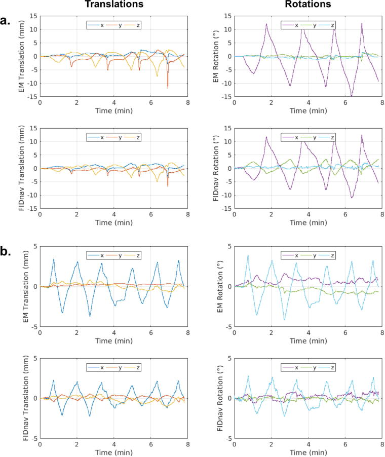
Translational and rotational motion trajectories estimated from the EM tracking system and the proposed FIDnav motion measurement system during a volunteer scan where the subject was verbally instructed to perform a smooth, continuous (a) nodding motion and (b) shaking motion for the duration of the scan. FIDnav motion estimates are in good agreement with the ground truth motion values measured by the EM tracking system, with a slight trend for underestimation of larger amplitude motions.
FIG. 6.
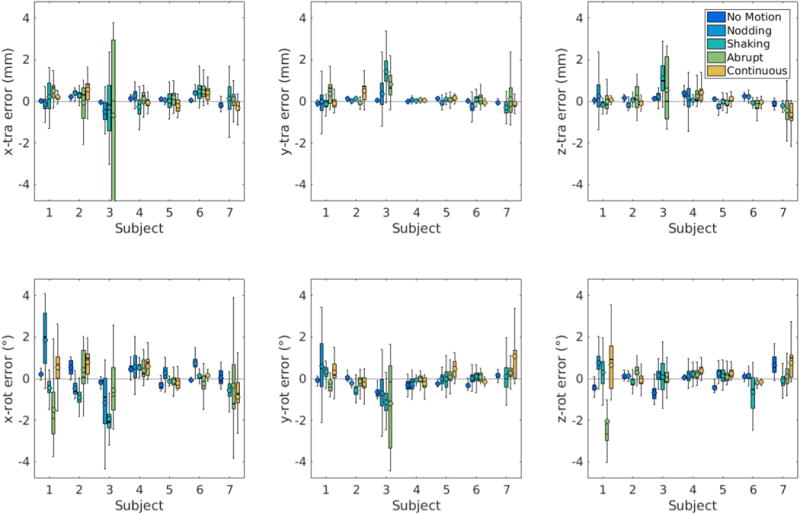
FIDnav motion prediction errors for all subjects and motion paradigms, plotted for translation and rotation about the x, y and z-axes. Boxplots visualize the distribution of the error and encapsulate data between the 25th (Q1) and 75th (Q3) percentiles i.e. the interquartile range (IQR), with the whiskers extending to the maximum errors not considered outliers (defined as data points further away from Q1 or Q3 by 1.5[IQR]). The median (solid line) and mean (open circle) errors are also shown. Overall, FIDnav motion predictions achieved good accuracy and precision, relative to the EM tracking system; however, larger errors are evident for some volunteers and motion paradigms.
The MVD computed within the masked brain region using rigid-body motion estimates from the EM tracker is shown in Figure 7 for each motion paradigm, along with the residual MVD following correction with FIDnav motion estimates. FIDnav-based correction resulted in a significant (P<0.05) decrease in MVD across all volunteers for each directed motion paradigm.
FIG. 7.
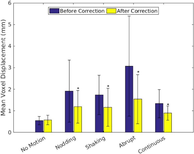
Summary of motion levels before and after FIDnav correction across different motion paradigms. MVD is calculated within the masked brain region from rigid-body motion estimates from the EM tracking system (blue bars). Yellow bars show the residual MVDs after correction with FIDnav motion estimates. FIDnav motion correction results in a significant (P<0.05; denoted by *) decrease in MVD across all volunteers and scans with intentional motion.
Retrospective Artifact Correction
Figure 8 shows a representative example of sagittal and axial slices through uncorrected and retrospectively corrected 3D FLASH images with abrupt intermittent head jerks, relative to the no motion scan, which acted as the reference image volume for comparison. Substantially reduced blurring can be seen with both EM and FIDnav-based motion compensation, with a corresponding increase in the SSIM index and decrease in NRMSE following correction. An example of retrospective correction of continuous free motion during acquisition of the central k-space lines is displayed in Figure 9, demonstrating a comparable improvement in image quality. Additional examples of FIDnav-based retrospective correction of abrupt and continuous motion are shown in Supporting Information Figures S6 and S7. Figure 10 shows improvements in NRMSE and SSIM indices with retrospective correction, compared to the uncorrected images for each motion paradigm. Across all subjects and scans with intentional motion, the NRMSE value of the uncorrected images was 6.11% ± 1.96%. Retrospective correction with the EM tracking and FIDnav motion estimates yielded significantly reduced (P<0.005) NRMSE values of 5.03% ± 1.52% and 5.11% ± 1.76%, respectively. A significant increase (P<0.01) in the SSIM index was also observed, from 0.773 ± 0.134 (uncorrected) to 0.818 ± 0.111 and 0.819 ± 0.125 with EM and FIDnav-based correction.
FIG. 8.
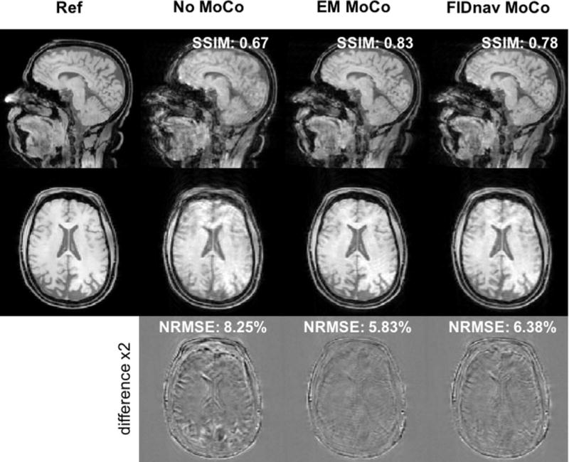
Impact of FIDnav-based retrospective correction of abrupt motion in Subject 1. Sagittal and axial slices through 3D FLASH images are shown (from left to right) with no voluntary motion, uncorrected image with abrupt motion, and with retrospective motion compensation using the EM tracking and FIDnav motion estimates. NRMSE and SSIM indices, relative to the reference scan, are also shown. FIDnav-based correction of abrupt head motion results in a comparable increase in both qualitative image quality and quantitative metrics, relative to ground-truth correction with EM tracking motion measurements.
FIG. 9.
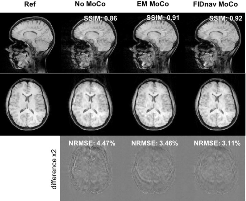
Impact of FIDnav-based retrospective correction of slow continuous motion during acquisition of the central k-space lines in Subject 5. Sagittal and axial slices through 3D FLASH images are shown (from left to right) with no voluntary motion, uncorrected image with slow, continuous motion, and with EM tracking and FIDnav-based retrospective motion compensation. FIDnavs provide accurate real-time motion estimates that can correct for continuous head motion, resulting in improved image quality.
FIG. 10.
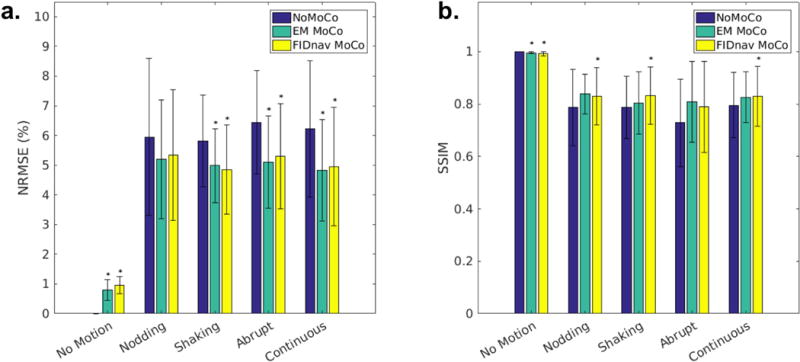
Improvement in quantitative image quality metrics with FIDnav-based retrospective correction. NRMSE in percent (a) and SSIM index (b) for each motion paradigm, relative to the uncorrected reference image acquired without any voluntary motion, before correction and after retrospective correction with EM tracking and FIDnav motion estimates. FIDnav-based motion compensation yielded a significant (P<0.05; denoted by *) improvement in NRMSE and SSIM across most motion paradigms tested.
DISCUSSION
This work describes a practical FIDnav-based motion measurement approach that eliminates the need for choreographed training with simultaneously acquired external tracking data by calibrating FIDnav measurements using simulated motion within a model of the head coil array. The effectiveness of this approach for retrospective motion compensation was demonstrated in a series of simulations and volunteer experiments with directed motion performed at 3T using a standard 32-channel head coil.
Numerical Simulations
Previous studies have assumed a linear relationship between FIDnav signal changes and underlying motion parameters (30,32,48); however, directly solving the inverse problem posed by measured FIDnavs failed to reliably estimate displacements and rotations >1 mm/° (48). Simulations revealed that whilst a simple linear regression model of FIDnav signals can account for small positional changes, the model breaks down at large amplitudes due to “cross-talk” between motion parameters, yielding poor accuracy and precision. Our proposed non-linear regression model can more effectively compensate for large motion amplitudes by accounting for second-order changes and interactions between parameters. In theory, even higher order models could be used, but at the risk of over-fitting parameters in the presence of noise. Rotations are more sensitive than translations to noise in the FIDnav time course and cross-talk errors, likely because translations induce larger FIDnav signal changes than rotations of equivalent magnitude. The simulations also revealed a trade-off between the resolution of the reference image and FIDnav tracking accuracy. The time taken to acquire the reference image should ideally be kept as short as possible, partly to minimize the potential for motion artifacts during this scan. In practice, a 4-mm resolution image provides an acceptable compromise between scan time and navigator accuracy.
Accuracy of Head Motion Measurement
Ground-truth motion values for intra-scan movement were provided by the EM tracking system. Overall, mean absolute translational and rotational errors were in the sub-millimeter and sub-degree range for motion amplitudes and patterns representative of those seen in less compliant subjects (16,49,50). The FIDnav prediction errors in this experiment were higher than those reported by Babayeva et al. (0.14 ± 0.21 mm and 0.08 ± 0.13°) for similar amplitude motions (32), likely due to the increased number of assumptions in using simulated data for the model calibration. The CSP extrapolation is expected to become less accurate further away from the original object boundaries, which may lead to errors when extrapolating larger amplitude motions. Furthermore, the FIDnav motion measurement model may break down in the presence of particularly large amplitude motion, due to changes in coil loading and motion-induced magnetic field (B0) variations, discussed in more detail below. Nevertheless, this is still a promising result as the previous study used a third of the acquired FIDnav and optical tracking data from each choreographed scan to train the regression algorithm, which is unrealistic in many clinical scenarios. Non-rigid motion, a lack of symmetry in the underlying coil geometry and inaccuracies in EM tracking (e.g. due to skin motion) are expected to be further sources of errors.
Retrospective Motion Correction with FIDnavs
Retrospective correction using the proposed FIDnav framework resulted in a comparable improvement in image quality, relative to ground-truth correction with EM tracking motion measurements, with substantially less blurring than the uncorrected images. Both EM tracking and FIDnav-based correction led to a significant decrease in NRMSE for all motion paradigms, except continuous head nodding. This may be due to artifacts caused by temporal B0 field variations, which are expected to be most severe for out-of-plane rotations. FIDnav motion compensation led to a significant increase in the SSIM index for all continuous motion paradigms; failure to achieve significance for abrupt motion may be due to the overall larger mean voxel displacements for this paradigm (Fig. 7). Residual artifacts are expected due to inconsistencies between k-space lines induced by large rotational motions, which is a limitation of retrospective correction without reacquisition of corrupted data.
Non-Rigid Motion
For the volunteer experiments, a multi-rigid approach (43) was employed for model calibration, to help compensate for the fact that the whole FOV does not move as a rigid body. This required manual definition of a binary mask to segment the head region (assumed to move rigidly) from the neck and shoulder region (assumed to remain stationary). Non-rigid motion e.g. swallowing (51) was also shown to influence FIDnav measurements, leading to small errors in motion estimation (Fig. 4). Future implementations could explore a more sophisticated model of head motion based on more realistic kinematic models and training with non-rigid motion. In this work, motion estimates were derived from FIDnavs measured from all 32 channels in the head coil array. Future work will explore the use of automated coil selection algorithms to help detect the dominant motion from a sub-set of coils and remove channels that are sensitive to noise and non-rigid motion (52). This could be particularly advantageous if using an even higher channel-count coil array.
B0 Field Variations
FIDnavs are sensitive to changes in B0 that arise due to thermal gradient drifts over time, respiration (53) and bulk motion (12). The former may be corrected by detrending the measured FIDnavs prior to motion estimation, but at the expense of reducing sensitivity to slow drift-like motion (30). Respiration is associated with both true motion as well as “apparent motion” induced by B0 variations attributed to bulk susceptibility changes in the lungs, and these effects can be difficult to resolve (54). As the main goal of this work was to correct for bulk rigid-body head motion, a low-pass filter was applied to the data to mitigate physiological fluctuations due to breathing and cardiac pulsation. Magnetic susceptibility boundaries produce distortions in the B0 field, which change as the subject moves. These changes are particularly important for out-of-plane rotations e.g. “nodding” motion due to the changing orientation of the object relative to the B0 field direction, which may confound motion measurements (12). In this work, only the magnitude of the FIDnavs was used as this primarily reflects changes in the distance to each coil element. Including phase values in the model gave a poor prediction performance, probably because of these phase effects that arise from position changes in susceptibility gradients, which are difficult to model. Previous work has demonstrated the ability of FIDnavs and sensitivity encoding to determine up to second-order B0 field inhomogeneities, with application for real-time shimming of the static magnetic field (55). Future work will test the ability of complex FIDnav signals to simultaneously monitor and correct for motion and temporal B0 fluctuations.
Timing Considerations
Whilst other image and k-space-based navigator approaches typically require sufficient dead time (on the order of hundreds of milliseconds) to be present in the host sequence, FIDnavs can be inserted into almost any sequence with just a marginal increase in the overall scan time. The same excitation pulse may be used for both navigation and imaging, so the minimal TE/TR is only increased by the duration of the navigator. To enable simulated training, the timing of the FIDnav is designed to match the contrast properties of the reference image. The minimal FIDnav duration is therefore limited by the minimum TE of the reference image and in theory could be further reduced by increasing the receiver bandwidth, decreasing the pixel resolution, or employing an ultra-short echo time 3D radial acquisition. Reducing the acquisition time of the FIDnav may also help reduce the confounding effects of B0 variations on motion estimates.
The simulated training step currently requires acquisition of two low-resolution reference scans (acquired using the surface and body coils, respectively) prior to imaging; however, these may also be useful in providing coil sensitivity information for subsequent sequences. Per-TR motion estimates can be obtained in ~10 ms, making this a feasible method for prospective motion correction. This would require CSP extrapolation and model calibration to be performed on-line. Significant speed-ups could be achieved by using fewer sample points to construct the CSP model and reducing the number of training data points. Further work would need to be done to assess the impact of each of these steps on the overall accuracy and precision of motion tracking.
Potential Applications
FIDnavs are an attractive approach for motion compensation in non-compliant subjects as motion data can be rapidly acquired, with minimal impact on contrast or scan time, using standard scanner hardware. Here, we demonstrate that our proposed approach may be used to measure a wide range of head motions with sub-millimeter and sub-degree accuracy and precision, and to retrospectively correct motion-corrupted 3D FLASH data with 1.3 mm in-plane resolution. In light of previous studies, which show that tracking accuracy should be on the order of a fraction of a pixel to ensure successful motion artifact correction (14), we suggest our proposed FIDnav motion measurement algorithm could be used to correct images with resolutions ~1 mm3, depending on the maximum observed motion amplitude. FIDnav motion measurements may also be used to guide autofocusing algorithms by providing an initial estimate and limiting the search space, making correction of higher-resolution 3D datasets more computationally feasible.
Extension to other non-selective 3D sequences should be relatively straightforward, providing a suitable low-resolution reference image can be acquired with the same contrast properties as the FIDnavs. The application of the proposed FIDnav motion measurement approach to 2D sequences is expected to be more challenging, as the acquired FIDnav will be sensitive to different excited spatial locations. This may be overcome by incorporating a model of the slice excitation profile into the simulations, but would require further experimentation to determine the validity of such an approach.
CONCLUSIONS
This work demonstrates the ability of our proposed motion measurement approach using FIDnavs and the spatial sensitivity patterns of multi-channel coil arrays to provide real-time, quantitative motion measurements for retrospective correction. In our implementation, the use of simulated training data eliminates the requirement for the subject to perform choreographed head movements prior to imaging, providing a more practical solution for motion compensation in less cooperative patient populations.
Supplementary Material
FIG. S1. Extrapolation of CSPs using global basis functions. Single slice through reference low-resolution surface coil image from a representative channel (a) and body coil image (b). Measured CSP computed from ratio of (a) and (b) in region masked by intensity thresholding of the body coil image (c). Sparse reliable data points selected by the first-order polynomial fitting test for the extrapolation (d). Extrapolated CSP over whole FOV using a 3D linear RBF (e). Absolute difference between measured (c) and extrapolated (e) CSP (f). RBF extrapolation from sparse reliable data points provides a good approximation of the CSPs across the whole FOV.
FIG. S2. Schematic showing calculation of FIDnav for locally rigid motion of the head. The low-resolution reference image is partitioned into fixed and rigidly moving parts by placing a single oblique plane to separate the head from the neck (and shoulder) region of the image. Rigid-body motion parameters are applied to the masked image shown in green and the simulated FIDnav signal is obtained by summing over both spatial regions.
FIG. S3. Motion tracking results for simulated 1D 10 mm/° motion steps estimated using linear (a) and non-linear (b) polynomial regression models (black), compared to ground truth motion, shown in gray. The non-linear model can more accurately predict large amplitude motion by accounting for interactions between parameters (reduced “cross-talk” errors).
FIG. S4. Measured FIDnavs during representative scans (Subject 1) with no voluntary motion (a), slow continuous nodding motion (b), slow continuous shaking motion (c), a series of eight abrupt head jerks (d) and continuous free motion during the central two minutes of the scan (e). Filtered FIDnavs (low-pass filter, cut-off frequency 0.2 Hz) are overlaid in black.
FIG. S5. Histograms showing distribution of the translational (left) and rotational (right) absolute errors of FIDnav motion estimates (relative to EM tracking measurements) across all subjects for each directed motion paradigm. Vertical bars show the 95th percentile of the measured motion amplitude in each direction.
FIG. S6. Additional example of FIDnav-based retrospective correction of abrupt motion in Subject 6. Sagittal and axial slices through 3D FLASH images are shown (from left to right) with no voluntary motion, uncorrected image with abrupt motion, and with retrospective motion compensation using the EM tracking and FIDnav motion estimates. NRMSE and SSIM indices, relative to the reference scan, are also shown.
FIG. S7. Additional example of FIDnav-based retrospective correction of slow continuous motion during acquisition of the central k-space lines in Subject 6. Sagittal and axial slices through 3D FLASH images are shown (from left to right) with no voluntary motion, uncorrected image with slow, continuous motion, and with EM tracking and FIDnav-based retrospective motion compensation.
Acknowledgments
This research was supported in part by the following NIH grant awards: R01 EB019483, R01 NS079788 and R44 MH086984.
APPENDIX
Radial Basis Function Extrapolation of Coil Sensitivity Profiles
RBFs provide a solution for interpolation or approximation of scattered data in multi-dimensional space. The scattered data interpolation problem can be formally described as follows. Given a set of function values at N distinct data points (nodes) , find an interpolant such that:
| [A1] |
where for points . Here, the function values are the measured CSPs (obtained by division of each low-resolution surface coil image by a body coil image), sampled at reliable data points within the original image (determined by a local first-order polynomial fitting criteria). The general form of an RBF consists of a set of N basis functions and weighting coefficients as follows:
| [A2] |
where is a low degree polynomial, added to help to regulate the matrix inversion and improve accuracy at domain boundaries. To remove the additional DOF, Equation A2 is subject to the following side conditions:
| [A3] |
Various choices exist for the basis function including polyharmonic, Gaussian and multi-quadric functions. The thin plate spline is a popular choice for fitting smooth functions for . In this work, we employ a linear RBF (biharmonic spline) , which has C1 continuity, to fit a smooth function in three dimensions. The weights and linear polynomial terms can be found by solving the following linear system of equations:
| [A4] |
The matrix form can be written as:
| [A5] |
Since noise is present in the measured CSP, the interpolation condition is too strict and can be relaxed by introducing a regularization term. A solution can then be found that approximates the data by minimizing the following cost function:
| [A6] |
where and denotes the semi-norm, which gives a measure of the energy or “smoothness” of the function. The regularization parameter controls the trade-off between smoothness and fidelity to the underlying data. This corresponds to introducing non-zero diagonal terms to the matrix in Equation A5 as follows:
| [A7] |
where I is the identity matrix. Thus, by solving the system of linear equations in Equation A7 a smooth extrapolation of the CSP is obtained across the whole FOV.
References
- 1.Zaitsev M, Maclaren J, Herbst M. Motion artifacts in MRI: A complex problem with many partial solutions. J Magn Reson Imaging. 2015;42:887–901. doi: 10.1002/jmri.24850. [DOI] [PMC free article] [PubMed] [Google Scholar]
- 2.Cote CJ, Wilson S. Guidelines for monitoring and management of pediatric patients during and after sedation for diagnostic and therapeutic procedures: an update. Pediatric Anesthesia. 2008;18:9–10. doi: 10.1111/j.1460-9592.2007.02404.x. [DOI] [PubMed] [Google Scholar]
- 3.Havidich JE, Beach M, Dierdorf SF, Onega T, Suresh G, Cravero JP. Preterm versus term children: Analysis of sedation/anesthesia adverse events and longitudinal risk. Pediatrics. 2016;137:e20150463. doi: 10.1542/peds.2015-0463. [DOI] [PMC free article] [PubMed] [Google Scholar]
- 4.Mansfield P. Multi-planar image formation using NMR spin echoes. J Phys C Solid State Phys. 1977;10:55–58. [Google Scholar]
- 5.Hennig J, Nauerth A. RARE imaging: A fast imaging method for clinical MR. Magn Reson Med. 1986;3:823–833. doi: 10.1002/mrm.1910030602. [DOI] [PubMed] [Google Scholar]
- 6.Sodickson DK, Manning WJ. Simultaneous acquisition of spatial harmonics (SMASH): Fast imaging with radiofrequency coil arrays. Magn Reson Med. 1997;38:591–603. doi: 10.1002/mrm.1910380414. [DOI] [PubMed] [Google Scholar]
- 7.Pruessmann KP, Weiger M, Scheidegger MB, Boesiger P. SENSE: Sensitivity encoding for fast MRI. Magn Reson Med. 1999;42:952–962. [PubMed] [Google Scholar]
- 8.Griswold MA, Jakob PM, Heidemann RM, Nittka M, Jellus V, Wang J, Kiefer B, Haase A. Generalized autocalibrating partially parallel acquisitions (GRAPPA) Magn Reson Med. 2002;47:1202–1210. doi: 10.1002/mrm.10171. [DOI] [PubMed] [Google Scholar]
- 9.Feinberg DA, Setsompop K. Ultra-fast MRI of the human brain with simultaneous multi-slice imaging. J Magn Reson. 2013;229:90–100. doi: 10.1016/j.jmr.2013.02.002. [DOI] [PMC free article] [PubMed] [Google Scholar]
- 10.Lustig M, Donoho D, Pauly JM. Sparse MRI: The application of compressed sensing for rapid MR imaging. Magn Reson Med. 2007;58:1182–1195. doi: 10.1002/mrm.21391. [DOI] [PubMed] [Google Scholar]
- 11.Godenschweger F, Kägebein U, Stucht D, Yarach U, Sciarra A, Yakupov R, Lüsebrink F, Schulze P, Speck O. Motion correction in MRI of the brain. Phys Med Biol. 2016;61:32–56. doi: 10.1088/0031-9155/61/5/R32. [DOI] [PMC free article] [PubMed] [Google Scholar]
- 12.Maclaren J, Herbst M, Speck O, Zaitsev M. Prospective motion correction in brain imaging: A review. Magn Reson Med. 2013;69:621–636. doi: 10.1002/mrm.24314. [DOI] [PubMed] [Google Scholar]
- 13.Aksoy M, Forman C, Straka M, Çukur T, Hornegger J, Bammer R. Hybrid prospective and retrospective head motion correction to mitigate cross-calibration errors. Magn Reson Med. 2012;67:1237–1251. doi: 10.1002/mrm.23101. [DOI] [PMC free article] [PubMed] [Google Scholar]
- 14.Maclaren J, Speck O, Stucht D, Schulze P, Hennig J, Zaitsev M. Navigator accuracy requirements for prospective motion correction. Magn Reson Med. 2010;63:162–170. doi: 10.1002/mrm.22191. [DOI] [PMC free article] [PubMed] [Google Scholar]
- 15.Qin L, Van Gelderen P, Derbyshire JA, Jin F, Lee J, De Zwart JA, Tao Y, Duyn JH. Prospective head-movement correction for high-resolution MRI using an in-bore optical tracking system. Magn Reson Med. 2009;62:924–34. doi: 10.1002/mrm.22076. [DOI] [PMC free article] [PubMed] [Google Scholar]
- 16.Afacan O, Erem B, Roby DP, Roth N, Roth A, Prabhu SP, Warfield SK. Evaluation of motion and its effect on brain magnetic resonance image quality in children. Pediatr Radiol. 2016;46:1728–35. doi: 10.1007/s00247-016-3677-9. [DOI] [PMC free article] [PubMed] [Google Scholar]
- 17.Ooi MB, Krueger S, Thomas WJ, Swaminathan SV, Brown TR. Prospective real-time correction for arbitrary head motion using active markers. Magn Reson Med. 2009;62:943–954. doi: 10.1002/mrm.22082. [DOI] [PMC free article] [PubMed] [Google Scholar]
- 18.Glover GH, Pauly JM. Projection reconstruction techniques for reduction of motion effects in MRI. Magn Reson Med. 1992;28:275–289. doi: 10.1002/mrm.1910280209. [DOI] [PubMed] [Google Scholar]
- 19.Meyer CH, Hu BS, Nishimura DG, Macovski A. Fast spiral coronary artery imaging. Magn Reson Med. 1992;28:202–213. doi: 10.1002/mrm.1910280204. [DOI] [PubMed] [Google Scholar]
- 20.Pipe JG. Motion correction with PROPELLER MRI: Application to head motion and free-breathing cardiac imaging. Magn Reson Med. 1999;42:963–969. doi: 10.1002/(sici)1522-2594(199911)42:5<963::aid-mrm17>3.0.co;2-l. [DOI] [PubMed] [Google Scholar]
- 21.Welch EB, Rossman PJ, Felmlee JP, Manduca A. Self-navigated motion correction using moments of spatial projections in radial MRI. Magn Reson Med. 2004;52:337–345. doi: 10.1002/mrm.20151. [DOI] [PubMed] [Google Scholar]
- 22.Liu C, Bammer R, Kim DH, Moseley ME. Self-navigated interleaved spiral (SNAILS): Application to high-resolution diffusion tensor imaging. Magn Reson Med. 2004;52:1388–1396. doi: 10.1002/mrm.20288. [DOI] [PubMed] [Google Scholar]
- 23.White N, Roddey C, Shankaranarayanan A, Han E, Rettmann D, Santos J, Kuperman J, Dale A. PROMO: Real-time prospective motion correction in MRI using image-based tracking. Magn Reson Med. 2010;63:91–105. doi: 10.1002/mrm.22176. [DOI] [PMC free article] [PubMed] [Google Scholar]
- 24.Gallichan D, Marques JP, Gruetter R. Retrospective correction of involuntary microscopic head movement using highly accelerated fat image navigators (3D FatNavs) at 7T. Magn Reson Med. 2016;75:1030–1039. doi: 10.1002/mrm.25670. [DOI] [PubMed] [Google Scholar]
- 25.Tisdall MD, Hess AT, Reuter M, Meintjes EM, Fischl B, Van Der Kouwe AJW. Volumetric navigators for prospective motion correction and selective reacquisition in neuroanatomical MRI. Magn Reson Med. 2012;68:389–399. doi: 10.1002/mrm.23228. [DOI] [PMC free article] [PubMed] [Google Scholar]
- 26.Welch EB, Manduca A, Grimm RC, Ward HA, Jack CR. Spherical navigator echoes for full 3D rigid body motion measurement in MRI. Magn Reson Med. 2002;47:31–41. doi: 10.1002/mrm.10012. [DOI] [PubMed] [Google Scholar]
- 27.Moriguchi H, Lewin JS, Duerk JL. Novel interleaved spiral imaging motion correction technique using orbital navigators. Magn Reson Med. 2003;50:423–428. doi: 10.1002/mrm.10507. [DOI] [PubMed] [Google Scholar]
- 28.Van Der Kouwe AJW, Benner T, Dale AM. Real-time rigid body motion correction and shimming using cloverleaf navigators. Magn Reson Med. 2006;56:1019–1032. doi: 10.1002/mrm.21038. [DOI] [PubMed] [Google Scholar]
- 29.Hu X, Kim S-G. Reduction of signal fluctuation in functional MRI using navigator echoes. Magn Reson Med. 1994;31:495–503. doi: 10.1002/mrm.1910310505. [DOI] [PubMed] [Google Scholar]
- 30.Kober T, Marques JP, Gruetter R, Krueger G. Head motion detection using FID navigators. Magn Reson Med. 2011;66:135–43. doi: 10.1002/mrm.22797. [DOI] [PubMed] [Google Scholar]
- 31.Waszak M, Falkovskiy P, Hilbert T, Bonnier G, Maréchal B, Meuli R, Gruetter R, Kober T, Krueger G. Prospective head motion correction using FID-guided on-demand image navigators. Magn Reson Med. 2017;78:193–203. doi: 10.1002/mrm.26364. [DOI] [PubMed] [Google Scholar]
- 32.Babayeva M, Kober T, Knowles B, Herbst M, Meuli R, Zaitsev M, Krueger G. Accuracy and precision of head motion information in multi-channel free induction decay navigators for magnetic resonance imaging. IEEE Trans Med Imaging. 2015;34:1879–1889. doi: 10.1109/TMI.2015.2413211. [DOI] [PubMed] [Google Scholar]
- 33.Keil B, Blau JN, Biber S, Hoecht P, Tountcheva V, Setsompop K, Triantafyllou C, Wald LL. A 64-channel 3T array coil for accelerated brain MRI. Magn Reson Med. 2013;70:248–258. doi: 10.1002/mrm.24427. [DOI] [PMC free article] [PubMed] [Google Scholar]
- 34.Hoult DI, Richards RE. The signal-to-noise ratio of the nuclear magnetic resonance experiment. J Magn Reson. 1976;24:71–85. doi: 10.1016/j.jmr.2011.09.018. [DOI] [PubMed] [Google Scholar]
- 35.Roemer PB, Edelstein WA, Hayes CE, Souza SP, Mueller M. The NMR phased array. Magn Reson Med. 1990;16:192–225. doi: 10.1002/mrm.1910160203. [DOI] [PubMed] [Google Scholar]
- 36.Faraji-Dana Z, Tam F, Chen JJ, Graham SJ. A robust method for suppressing motion-induced coil sensitivity variations during prospective correction of head motion in fMRI. Magn Reson Imaging. 2016;34:1206–1219. doi: 10.1016/j.mri.2016.06.005. [DOI] [PubMed] [Google Scholar]
- 37.Moyher SE, Vigneron DB, Nelson SJ. Surface coil MR imaging of the human brain with an analytic reception profile correction. J Magn Reson Imaging. 1995;5:139–44. doi: 10.1002/jmri.1880050204. [DOI] [PubMed] [Google Scholar]
- 38.Dawant BM, Zijdenbos AP, Margolin RA. Correction of intensity variations in MR images for computer-aided tissue classification. IEEE Trans Med Imaging. 1993;12:770–781. doi: 10.1109/42.251128. [DOI] [PubMed] [Google Scholar]
- 39.Guerquin-Kern M, Lejeune L, Pruessmann KP, Unser M. Realistic analytical phantoms for parallel magnetic resonance imaging. IEEE Trans Med Imaging. 2012;31:626–636. doi: 10.1109/TMI.2011.2174158. [DOI] [PubMed] [Google Scholar]
- 40.Cocosco CA, Kollokian V, Kwan RKS, BrainWeb ACE. Online Interface to a 3D MRI Simulated Brain Database [Google Scholar]
- 41.Powell MJD. The BOBYQA algorithm for bound constrained optimization without derivatives. Cambridge, UK: 2009. [Google Scholar]
- 42.Lai SH, Fang M. A dual image approach for bias field correction in magnetic resonance imaging. Magn Reson Imaging. 2003;21:121–125. doi: 10.1016/s0730-725x(02)00637-9. [DOI] [PubMed] [Google Scholar]
- 43.Loktyushin A, Nickisch H, Pohmann R, Scholkopf B. Blind multirigid retrospective motion correction of MR images. Magn Reson Med. 2015;73:1457–1468. doi: 10.1002/mrm.25266. [DOI] [PubMed] [Google Scholar]
- 44.Umeyama S. Least-Squares Estimation of Transformation Parameters Between Two Point Patterns. IEEE Trans Pattern Anal Mach Intell. 1991;13:376–380. [Google Scholar]
- 45.Maclaren J, Aksoy M, Ooi MB, Zahneisen B, Bammer R. Prospective motion correction using coil-mounted cameras: Cross-calibration considerations. Magn Reson Med. 2018;79:1911–1921. doi: 10.1002/mrm.26838. [DOI] [PMC free article] [PubMed] [Google Scholar]
- 46.Fessler JA. [accessed September 2017];Michigan Image Reconstruction Toolbox. https://web.eecs.umich.edu/~fessler/code.
- 47.Wang Z, Bovik AC, Sheikh HR, Simoncelli EP. Image quality assessment: From error visibility to structural similarity. IEEE Trans Image Process. 2004;13:600–612. doi: 10.1109/tip.2003.819861. [DOI] [PubMed] [Google Scholar]
- 48.Kober T, Marques JP, Gruetter R, Krueger G. Motion characterisation using FID navigators and spatial pattern of MRI coil arrays. Proc Int Soc Magn Reson Med. 2010:3047. [Google Scholar]
- 49.Lemieux L, Salek-Haddadi A, Lund TE, Laufs H, Carmichael D. Modelling large motion events in fMRI studies of patients with epilepsy. Magn Reson Imaging. 2007;25:894–901. doi: 10.1016/j.mri.2007.03.009. [DOI] [PubMed] [Google Scholar]
- 50.Brown TT, Kuperman JM, Erhart M, White NS, Roddey JC, Shankaranarayanan A, Han ET, Rettmann D, Dale AM. Prospective motion correction of high-resolution magnetic resonance imaging data in children. Neuroimage. 2010;53:139–145. doi: 10.1016/j.neuroimage.2010.06.017. [DOI] [PMC free article] [PubMed] [Google Scholar]
- 51.Dyverfeldt P, Deshpande VS, Kober T, Krueger G, Saloner D. Reduction of motion artifacts in carotid MRI using free-induction decay navigators. J Magn Reson Imaging. 2014;40:214–220. doi: 10.1002/jmri.24389. [DOI] [PMC free article] [PubMed] [Google Scholar]
- 52.Zhang T, Cheng JY, Chen Y, Nishimura DG, Pauly JM, Vasanawala SS. Robust self-navigated body MRI using dense coil arrays. Magn Reson Med. 2016;76:197–205. doi: 10.1002/mrm.25858. [DOI] [PMC free article] [PubMed] [Google Scholar]
- 53.Van de Moortele PF, Pfeuffer J, Glover GH, Ugurbil K, Hu X. Respiration-induced B0 fluctuations and their spatial distribution in the human brain at 7 tesla. Magn Reson Med. 2002;47:888–895. doi: 10.1002/mrm.10145. [DOI] [PubMed] [Google Scholar]
- 54.Gretsch F, Marques JP, Gallichan D. Investigating the accuracy of FatNav-derived estimates of temporal B0 changes and their application to retrospective correction of high-resolution 3D GRE of the human brain at 7T. Magn Reson Med. 2018;0 doi: 10.1002/mrm.27063. [DOI] [PubMed] [Google Scholar]
- 55.Splitthoff DN, Zaitsev M. SENSE shimming (SSH): A fast approach for determining B0 field inhomogeneities using sensitivity coding. Magn Reson Med. 2009;62:1319–1325. doi: 10.1002/mrm.22083. [DOI] [PubMed] [Google Scholar]
Associated Data
This section collects any data citations, data availability statements, or supplementary materials included in this article.
Supplementary Materials
FIG. S1. Extrapolation of CSPs using global basis functions. Single slice through reference low-resolution surface coil image from a representative channel (a) and body coil image (b). Measured CSP computed from ratio of (a) and (b) in region masked by intensity thresholding of the body coil image (c). Sparse reliable data points selected by the first-order polynomial fitting test for the extrapolation (d). Extrapolated CSP over whole FOV using a 3D linear RBF (e). Absolute difference between measured (c) and extrapolated (e) CSP (f). RBF extrapolation from sparse reliable data points provides a good approximation of the CSPs across the whole FOV.
FIG. S2. Schematic showing calculation of FIDnav for locally rigid motion of the head. The low-resolution reference image is partitioned into fixed and rigidly moving parts by placing a single oblique plane to separate the head from the neck (and shoulder) region of the image. Rigid-body motion parameters are applied to the masked image shown in green and the simulated FIDnav signal is obtained by summing over both spatial regions.
FIG. S3. Motion tracking results for simulated 1D 10 mm/° motion steps estimated using linear (a) and non-linear (b) polynomial regression models (black), compared to ground truth motion, shown in gray. The non-linear model can more accurately predict large amplitude motion by accounting for interactions between parameters (reduced “cross-talk” errors).
FIG. S4. Measured FIDnavs during representative scans (Subject 1) with no voluntary motion (a), slow continuous nodding motion (b), slow continuous shaking motion (c), a series of eight abrupt head jerks (d) and continuous free motion during the central two minutes of the scan (e). Filtered FIDnavs (low-pass filter, cut-off frequency 0.2 Hz) are overlaid in black.
FIG. S5. Histograms showing distribution of the translational (left) and rotational (right) absolute errors of FIDnav motion estimates (relative to EM tracking measurements) across all subjects for each directed motion paradigm. Vertical bars show the 95th percentile of the measured motion amplitude in each direction.
FIG. S6. Additional example of FIDnav-based retrospective correction of abrupt motion in Subject 6. Sagittal and axial slices through 3D FLASH images are shown (from left to right) with no voluntary motion, uncorrected image with abrupt motion, and with retrospective motion compensation using the EM tracking and FIDnav motion estimates. NRMSE and SSIM indices, relative to the reference scan, are also shown.
FIG. S7. Additional example of FIDnav-based retrospective correction of slow continuous motion during acquisition of the central k-space lines in Subject 6. Sagittal and axial slices through 3D FLASH images are shown (from left to right) with no voluntary motion, uncorrected image with slow, continuous motion, and with EM tracking and FIDnav-based retrospective motion compensation.


