

Abstract
Purpose
To improve the depiction and tracking of vocal tract articulators in spiral real-time magnetic resonance imaging (RT-MRI) of speech production, by estimating and correcting for dynamic changes in off-resonance.
Methods
The proposed method computes a dynamic field map from the phase of single-TE dynamic images after a coil phase compensation where complex coil sensitivity maps are estimated from the single-TE dynamic scan itself. This method is tested using simulations, and in-vivo data. The depiction of air-tissue boundaries is evaluated quantitatively using a sharpness metric, and using visual inspection.
Results
Simulations demonstrate that the proposed method provides robust off-resonance correction for spiral readout durations up to 5 ms at 1.5 Tesla. In-vivo experiments during human speech production demonstrate that image sharpness is improved in a majority of datasets at air-tissue boundaries including the upper lip, hard palate, soft palate, and tongue boundaries, while the lower lip shows little improvement in the edge sharpness after correction.
Conclusion
Dynamic off-resonance correction is feasible from single-TE spiral RT-MRI data, and provides a practical performance improvement in articulator sharpness when applied to speech production imaging.
Keywords: off-resonance correction, real-time MRI, speech production, spiral
INTRODUCTION
Real-time magnetic resonance imaging (RT-MRI) has become a valuable tool for speech production research (1–3) and is now a preferred tool in speech science to alternative imaging modalities including x-ray microbeam (4), electromagnetic articulography (5), and ultrasound (6). RT-MRI provides a non-invasive capture of the dynamics of deep articulatory structures (e.g., pharynx, glottis and epiglottis) during speech production and allows for arbitrary imaging planes. In this context, spiral RT-MRI scanning is desirable because it allows for a time efficient acquisition, given that spirals can provide higher spatio-temporal resolution than alternative schemes (1).
A key drawback of spiral MRI is signal loss and/or blurring artifacts that result from field inhomogeneity, also called “off-resonance” (7). This can be significant at air-tissue interfaces due to their magnetic susceptibility difference ( = 9.41 parts per million) (8). Furthermore, these artifacts near the air-tissue boundaries (9) are more pronounced with long spiral readout or at high field strength MRI scanners. To mitigate this artifact, current RT-MRI studies for speech production are most often conducted using short duration readouts (~2.5 ms) and at lower field strength (1.5 Tesla (T)) MRI scanners (10–12).
Off-resonance artifacts have significant potential impact on the analysis of articulator dynamics, which is of prime interest in speech science. The articulators of interest include the surfaces of the lips, tongue, hard palate, soft palate (velum), and structures along the pharyngeal airway. These are located at air-tissue interfaces and therefore are vulnerable to the artifacts. Previously used speech RT-MRI biomarkers, such as average pixel intensity (13,14) in regions of interest (ROI) are prone to error due to artefactual airway area perturbation. Any temporally varying blur of soft tissues can result in changes in the detected patent airway, and will disrupt the estimation of constriction kinematics, such as timing in consonant production (13). Air-tissue boundary segmentation (15–17) is required as a pre-processing step in acquiring vocal tract area functions (18) and suffers in the presence of ambiguous boundaries with poor contrast. Velopharyngeal insufficiency (19–23) is caused by incomplete closure between the soft palate and the posterior and lateral pharyngeal walls, and its assessment can be hampered by signal loss near the soft palate.
Several deblurring methods in spiral scanning have been proposed in the literature (24–30), most of which require a measurement of a frequency offset image, also called a “field map” (24–26). A previous study applied this approach to spiral RT-MRI of vocal tract (31) where spirals with two different echo times (TEs) were obtained in an interleaved fashion and a dynamic field map was estimated using each pair of consecutive images. This field map-based method showed improvement of image quality in the tongue and soft palate. The reconstructed images, however, could suffer from flickering artifact between consecutive images reconstructed with different TEs. This scheme also requires a compromise in temporal and/or spatial resolution (31) and is not applicable to previously-collected single-echo-time data.
An alternative approach is to estimate the field map directly from the dataset itself, known as “auto-focus” (27–30). Auto-focus methods employ an image-domain focus metric that provides local information about the presence of residual off-resonance artifacts based on the off-resonance point spread function (PSF). A widely used metric is the absolute value of the imaginary component of the image (after correcting for a coil phase) at an image location (28). It assumes that the imaginary component should be zero when the local effects of off-resonance have been corrected. These methods have shown comparable results to the methods that acquire the field map. However, these are computationally demanding and performance depends on the focus metric used and can be sensitive to experimental factors, such as MRI sequence parameters, signal-to-noise ratio (SNR), and the accuracy of coil sensitivity maps (especially their phase). Additionally, spurious minima of the focus metric can occur as the range of off-resonance at air-tissue interfaces (~600 Hz at 1.5 T) is large enough to produce more than one cycle of phase accrual (>2π) even during a short spiral readout (~2.5 ms) (27,32,33).
In this work, we present a simple dynamic off-resonance estimation method for spiral imaging where a dynamic field map is directly estimated from the phase of single-TE dynamic images after a coil phase compensation. We estimate complex coil sensitivity map from the single-TE scan itself. Our approach does not require a dynamic two-echo measurement of a field map, nor the use of a focus metric. Therefore, it can be performed on conventional real-time spiral data without the need for additional scanning and is not computationally intensive. We evaluate this method using simulations and on an existing multi-speaker dataset of running speech. We demonstrate improvements in the depiction of air-tissue boundaries quantitatively using an image sharpness metric, and using visual inspection, and the practical utility of this method on a use case.
THEORY
Spiral Imaging in the Presence of the Field Inhomogeneity
In spiral MRI, ignoring relaxation and noise, the signal equation of an object with a transverse magnetization is given by
| [1] |
where is time variable defining =0 as the start of the readout; is the readout duration. r and are the spatial coordinate and the k-space trajectory, respectively. ; is the off-resonance frequency presented at r; is the complex coil sensitivity map.
Consider the image signal ( ) reconstructed from without off-resonance correction as follows:
| [2] |
where is a PSF of an imaging system using a particular k-space trajectory in the presence of ; denotes the pre-density compensation function for the trajectory. When , we can ignore a phase accrual due to off-resonance during the readout. Then, the PSF in Eq. [2] is a sharp impulse at so that the image signal in Eq. [2] can be approximated by .
Field Map Estimation in Spiral Imaging
Consider spiral RT-MRI, where the image time series ( ) for i-th coil is:
| [3] |
where t represents time frame; is dynamic off-resonance; is the complex coil sensitivity map that is spatially smooth and independent of time. Phase accrual during the spiral readout is ignored. Assuming that is real, we can compute an estimate of the dynamic field map, , as follows:
| [4] |
where denotes a coil-composite image using the optimal B1 combination (34), which is given by
| [5] |
here is an estimate of the sensitivity maps, is the number of coil components; is the complex conjugate of .
METHODS
Implementation of Field Map Estimation for Speech RT-MRI
Figure 1 illustrates the proposed field map estimation process. The individual coil image frames are first reconstructed from raw k-space using sliding window view-sharing with the nonuniform fast Fourier transform (NUFFT) (35). For sliding window view-sharing, reconstructions were performed every 4 spirals using a temporal window of 13 spirals (fully sampled k-space). Note that this number matches to a frame rate of dynamic images to be reconstructed in off-resonance correction, which will be described more in the “Off-resonance Correction” section. The multi-coil images are then merged into composite image frames based on Eq. [5] using complex coil sensitivity maps, whose estimation will be discussed later. is then smoothed by convolution with a 3D Hanning window (r-t) with size 3 3 3 to reduce noise, and masked by either of 0 or 1 based on a threshold (2% of maximum of the absolute squared value of the smoothed image) to control uninitialized values in air spaces that result from a lack of image signal. Consequently, a dynamic field map is estimated from the smoothed and masked images of based on Eq. [4].
Figure 1.
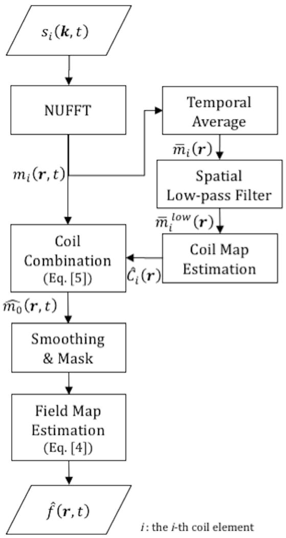
Flow-chart illustrating the proposed field map estimation method. The raw image frames from individual coils are first reconstructed from the raw k-space data using view-sharing with NUFFT. The coil sensitivity maps are estimated from the multi-coil image frames after temporal average and spatial low-pass filter. The multi-coil image frames are then merged into composite image frames using the complex coil maps by Eq. [5]. The composite images are smoothed and masked and a dynamic field map is estimated from the phase of the resulting image frames by Eq. [4].
Complex coil sensitivity maps (the ‘i’ subscript indicates the i-th coil element) are estimated from a temporally averaged and spatially low-pass filtered image. The individual coil image frames (shown in Figure 1) are averaged over time and low-pass filtered by a 2D Hanning window with size 15 15 pixels (FWHM 8 pixels). Note that this low-pass filter is different from the smoothing applied to and is comparable to a low-pass filter that takes 12.5% of the central part of the k-space. These settings were chosen empirically. Then, the resultant image is used to estimate the coil map by . A drawback of this approach is that the spatially smooth portion of the time-averaged field map will be spuriously included in the coil sensitivity map, and will not be corrected, which will be extensively discussed in the “Discussion” section.
Simulation
To assess the accuracy of the proposed field map estimation, a simulation was performed with various spiral readout durations as follows: Cartesian images with two TEs (ΔTE = 1 ms) were acquired from a healthy subject at 5 postures including mouth open at varying angles such as mouth fully open and mouth half open, mouth closed, and tongue tip raised to the front of the palate. For each of the postures, a reference field map was obtained from the phase difference between the images acquired at two TEs divided by ΔTE shown in Figure 2(a). Then, for a given spiral trajectory, spiral k-space data were synthesized from the magnitude of the Cartesian image from the first TE based on Eq. [1]. The reference field map was used to simulate off-resonance effects on the synthesized spiral k-space data. Those data simulations were performed with different readout durations varying from 0 ms to 6.3 ms with 0.63 ms increment. Finally, we estimated a field map from the simulated data and attempted to correct for off-resonance based on the estimated field map.
Figure 2.
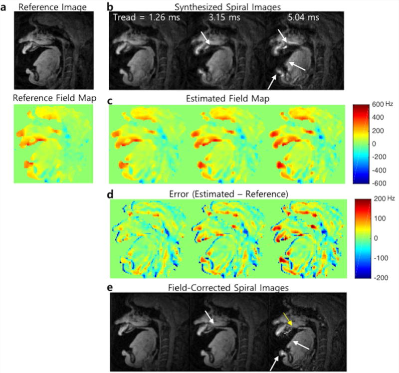
Representative simulation results. (a) A magnitude image and reference field map acquired from Cartesian dual-TE acquisition. (b) Synthesized spiral images using the magnitude image and reference field map with different readout durations (1.26, 3.15, and 5.04 ms). Off-resonance blurring is most apparent near the lips, hard palate, and tongue boundary and becomes worse with the longer readouts. (c) Field maps (Unit: Hz) estimated from phase of the spiral complex images shown in (b). (d) Estimation errors in the field map (error maps amplified by a factor of 3 for better visualization). (e) Spiral images after correction for off-resonance based on the estimated field map represented in (c).
Application to Existing Speech RT-MRI Data
Experiments were performed on a speech RT-MRI dataset collected at our institution using a standardized vocal-tract protocol (36). It currently contains more than twenty healthy subjects’ data on a wide variety of speech tasks to capture salient, static and dynamic, articulatory characteristics of speech production as well as morphological aspects of the vocal tract (36). Notice that the degree of blurring artifacts in their images varies depending on the subjects and speech tasks. We selected twenty subjects (n = 20, 10F/10M; age 19 – 31 years) with several speech tasks from the dataset.
Imaging was performed using a real-time interactive imaging platform (RT-Hawk, Heart Vista Inc, Los Altos, CA) (37) on a commercial 1.5 T scanner (Signa Excite, GE Healthcare, Waukesha, WI). The body coil was used for RF transmission, and a custom eight-channel upper airway coil (12) was used for signal reception. A 13-interleaf spiral spoiled gradient echo pulse sequence was used. Imaging was performed in the mid-sagittal plane. Imaging parameters used were: = 2.52 ms, spatial resolution = 2.4 2.4 mm2, slice thickness = 6 mm, field of view (FOV) = 200 200 mm2, repetition time (TR) = 6.004 ms, TE = 0.8 ms, receiver bandwidth = ±125 kHz, and flip angle = 15 . In addition to the automatic shimming provided by the prescan calibration from the scanner, we performed a manual adjustment of the center frequency as described in Refs (1,12). Specifically, we on-the-fly adjusted the center frequency in a way that air-tongue boundary is sharp in the mid-sagittal plane while the subject being scanned is in a neutral open-mouth position.
Off-resonance Correction
We utilize an iterative approach (38,39) where the off-resonance exponential term is approximated by a set of bases to improve computational speed and to reconstruct a deblurred image. We integrate this approach into a recent sparse-SENSE reconstruction method (12) that utilizes temporal finite difference constraint to improve time resolution in the time-series of spiral images of speech. Specifically, off-resonance exponential term shown in Eq. [1] is approximated by non-exponential bases at each time frame, by using histogram principal components (K=40 bins) and singular value decomposition analysis (L=6) described in Eq. [19, 20] from Ref. (39). Then the approximated bases are incorporated into the imaging model used in the sparse-SENSE reconstruction (12). Raw k-space data and an estimated coil map are then fed into the reconstruction algorithm as inputs. In turn, it generates a corrected time-series of images. For evaluating the effectiveness of off-resonance correction, the original time-series of images were also reconstructed using the sparse-SENSE reconstruction without the modification. All the images were reconstructed with a temporal resolution of 24 ms/frame (41.66 frames/s, 4 spiral interleaves/frame, and with reduction factor R = 3.25). For implementation, a nonlinear conjugate gradient (CG) algorithm with NUFFT was coded using MATLAB (The MathWorks, Inc., Natick, MA) on using 8 cores on a 16-core Intel(R) Xeon(R) CPU E5-2698 v3; 2.30GHz, with 40 MB of L3 cache. The computation time was ~ 60 s to estimate the coil sensitivity maps and the field maps for 400 time frames from raw k-space data (~10 s long dynamic images) and 30 and 180 mins to reconstruct images without and with off-resonance correction, respectively.
Sharpness Score
We introduce an image sharpness measure to investigate the impact of the proposed method on articulator air-tissue boundaries. We quantitatively compare the metric scores between the images with and without correction. We hypothesize that the proposed method would improve the image depiction at air-tissue articulator boundaries in two ways – the blurred-edge width be narrowed and/or the contrast at the edge be enhanced. We define an edge-slope metric for sharpness as follows:
Using a semi-automatic boundary extraction method (16), we extract the superior-posterior (upper) boundary and the inferior-anterior (lower) boundary as shown in Figure 3(a). Then, intensity profiles (grid lines) perpendicular to the upper and lower boundary (Figure 3(b)) of the patent airway are chosen and extracted from a reconstructed image series with a normalized intensity between 0 and 1, and linearly interpolated to generate ten times greater spatial resolution. Finally, the sharpness score (S) is calculated (Figure 3(c)) as follows;
| [6] |
where is a scaling factor associated with the intensity normalization, , and ; and are points (nearby the extracted boundary pixel location) at 80% and 20% of the maximum intensity value in grid lines, respectively; I(p) is an intensity value at point p; is the standard deviation of an ROI outside the object where there is no signal. The sharpness score was calculated over valid time frames in which a distance between upper and lower boundary pixel locations is greater than 5 pixels. The sharpness score was compared using paired t-tests for statistical analysis, assuming that the samples collected along the grid lines are uncorrelated. A P value of <0.001 was used to determine statistical significance.
Figure 3.
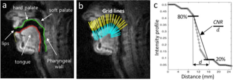
Illustration of articulator boundary identification and sharpness score evaluation. (a) Airway boundary segmentation with the upper (superior-posterior) boundary (green, color online) and the lower (inferior-anterior) boundary (red, color online). (b) Gridlines of the upper (yellow) and lower boundaries (cyan) at several locations along the airway are chosen to obtain intensity profiles. (c) Intensity profile of the gridline is plotted where a sharpness metric is measured as a slope between the points of 80% and 20% of the maximum intensity values (CNR/d).
Practical Utility of the Off-resonance Correction
Finally, in order to determine the practical utility of the off-resonance correction on an end use case, we measure vocal tract distance, which is a desired metric that is often used in the speech RT-MRI analysis to obtain constriction degree (40–42) or vocal tract area function (43–45). The distance metric is defined as the physical distance between the upper and lower boundaries shown in Figure 3(a). The boundaries are extracted using the aforementioned method (16) with the same initialization in both sets of images, without and with off-resonance correction. Distances were measured from both images.
RESULTS
Simulation
Figure 2 shows a representative example (static posture with mouth fully opened) of simulation results with different spiral readout durations. Off-resonance blurring is seen most clearly at the lips, hard palate, and tongue boundary and becomes more severe with the longer readouts as shown in Figure 2(b). As the duration of the readout is longer, the estimated field maps (Figure 2(c)) tend to be blurred and amplified in some areas such as the tongue surface and lips surface. Accordingly, high spatial frequency error can be seen in those area (Figure 2(d)). The estimated field map fails to correct for the simulated off-resonance for the longer readout duration (> 5 ms) and the blurred anatomical structures remain unresolved.
Existing Speech RT-MRI Data
Figure 4 contains representative mid-sagittal image frames and the corresponding field map estimated for four subjects, which, on visual assessment, presented the most significant blurring artifacts among the twenty subjects. Note that subject numbers of 4, 6, 9, and 13 shown in Figure 4 correspond to those shown in Figure 5. For every image reconstructed with off-resonance correction, the soft palate, hard palate, and medial surface of the tongue become more intense and sharper compared to the blurred images (see yellow arrows). For all the four subjects, posterior to the alveolar ridge, the hard palate appears sharper up to the soft palate in the deblurred images. Correspondingly, in the estimated field maps, the regions that have shown blurred anatomical structures represent high off-resonance frequency values of > 200 Hz.
Figure 4.
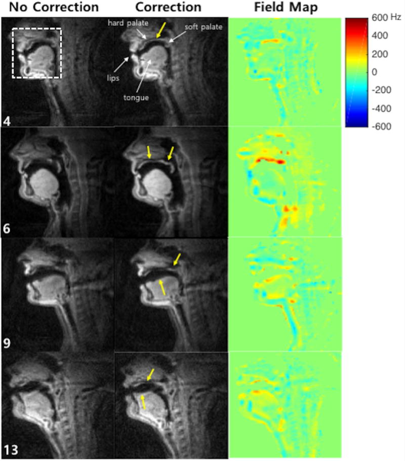
Representative mid-sagittal image frames of vocal tracts for four subjects, which, on visual assessment, presented the most significant blurring artifacts and were selected among the twenty subjects. The first and the second columns show images reconstructed with no correction and with correction, respectively. The last column shows the estimated field maps corresponding to those image time frames. Yellow arrows point out the regions that are most affected by off-resonance blurring, and corrected by the proposed method. (Video file is also available online as a supporting material.)
Figure 5.
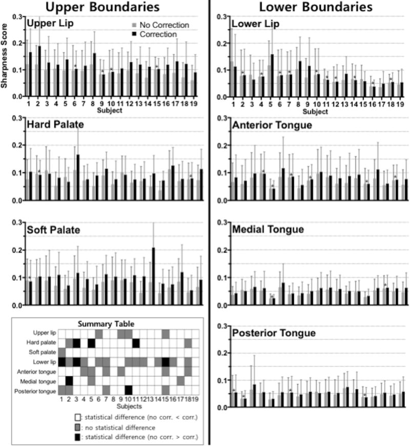
Sharpness without and with correction at different articulator boundary locations. Sharpness scores are measured at the upper boundaries (upper lip, hard palate, and soft palate) and lower boundaries (lower lip, anterior-, medial-, and posterior-tongue) along time. The mean and the standard deviation of the sharpness scores over time are shown here where the nineteen subjects are presented in descending order of average uncorrected sharpness score. A paired t-test was performed at each articulator boundary for each individual subject to test for the significance of the sharpness difference. The sharpness scores marked with an asterisk (*) were not found to be statistically different. All remaining scores were found to have significant mean differences (P < 0.001). Summary table in the bottom left panel summarizes the significance of mean sharpness score difference between no correction and correction in three different categories: (white) no correction < correction, (gray) no significant difference between no correction and correction, and (black) no correction > correction.
Figure 6 shows the profiles that are extracted at the solid lines in the sample image frames from the three subjects. For Subject 9, the intensity profile from the deblurred image provides a clear delineation of the soft palate movements. For Subjects 6 and 13, the intensity in the hard palate in the deblurred image sequence is more constant along time than the intensity value in the blurred image sequence. This result agrees with the fact that the hard palate, which is a bony structure covered by a thin layer of tissue, does not change its shape during speech production (17). Furthermore, the intensity profile from the deblurred image exhibits sharper boundary between tongue and air.
Figure 6.
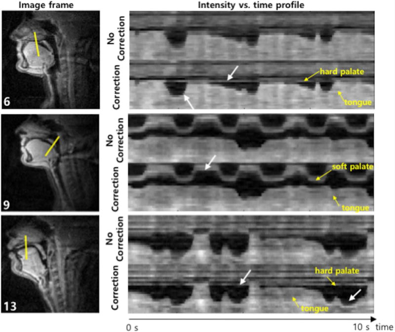
Illustration of improved sharpness of articulator boundaries. The first column shows an example frame for three different subjects and the second column shows intensity vs. time profiles marked by the solid lines in the first column images where each of the solid lines corresponds to one of the gridlines shown in Figure 3. For all subjects, the intensity time profiles from image sequences reconstructed with correction exhibit sharper boundary between tongue and air than that from image sequences with no correction. For Subject 9, the intensity profile from the correction provides a clear delineation of the soft palate movements. For Subjects 6 and 13, the correction method provides more constant intensity in the hard palate along time than image sequence with no correction.
Figure 7 illustrates one more example of correction result from Subject 4, especially showing the estimated field map over time. As depicted in the off-resonance frequency value vs. time profile, the proposed method enables capturing of the dynamic change in off-resonance at the tissue boundaries. Whereas the estimated field map shows high off-resonance frequency values at the hard palate and tongue boundaries over time, it shows a low frequency value at those boundaries during the event of the tongue touching the hard palate because there is no air between the tongue and hard palate (see white arrows).
Figure 7.
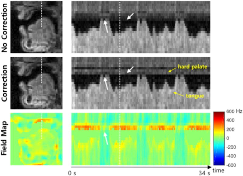
Illustration of the estimated field map over time. The first column shows example frames of reconstructed images and field map corresponding to the white dot box shown in Figure 4. The second column shows intensity vs. time profiles marked by the dot lines in the first column images. In the estimated field map, high off-resonance frequency values are shown at the hard palate (400 Hz) and tongue (200 Hz) boundaries over time except when the tongue contacts the hard palate. This is because when the tongue touches the hard palate, there is neither air and susceptibility difference between them. (Video file is available online as a supporting material.)
Sharpness Score
Figure 5 illustrates the sharpness scores and summary table. Sharpness scores without and with correction were measured at upper airway boundaries (upper lip, hard palate, and soft palate) and lower boundaries (lower lip, anterior-, medial-, and posterior-tongue) described in Figure 3 and averaged over time. The boundary extraction method used failed to segment the image from one subject due to low image quality, which was excluded in this sharpness analysis. Overall, the sharpness scores show a statistically significant difference in mean values (correction > no correction, P > 0.001) for the subjects tested at a majority of the boundaries. The lower lip shows negligible sharpness improvement in ten subjects and worse sharpness score in three subjects when correction was applied. The hard palate exhibits worse sharpness score in three subjects after correction compared to no correction, whereas fifteen subjects show improvement in sharpness score after correction.
Practical Utility of the Off-resonance Correction
Figure 8 illustrates airway boundary segmentation result based on which the corresponding vocal tract distance measured from images without and with correction from Subject 6 shown in Figure 4. The uncorrected image exhibits noticeable errors in the segmentation due to off-resonance-induced blurring around the hard palate and soft palate, as indicated with arrows in Figure 8(a) and erroneous results on the corresponding vocal tract distance in those area as shown in Figure 8(b).
Figure 8.
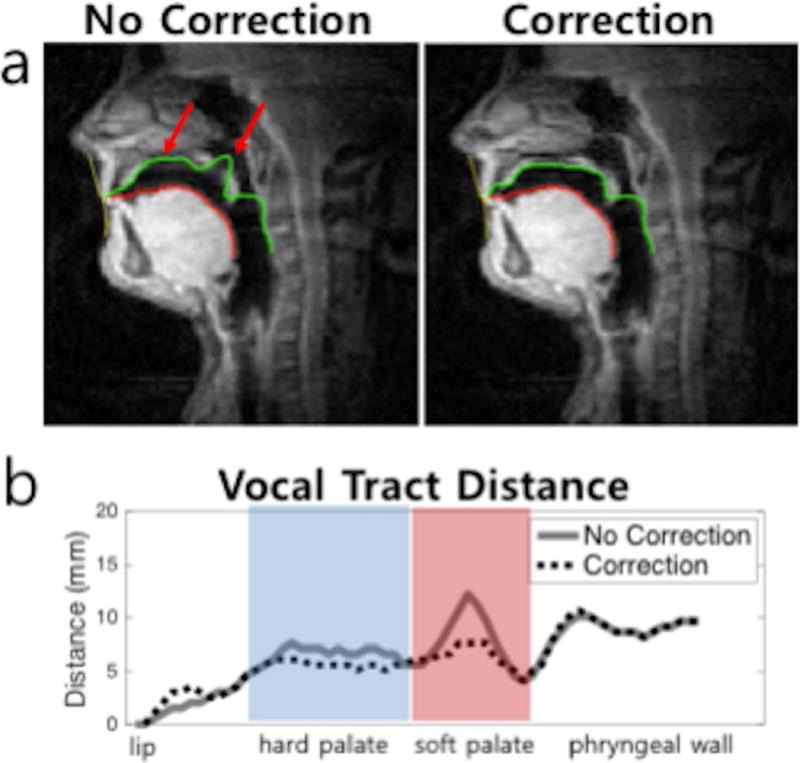
Representative illustration of airway boundary segmentation results on images without and with correction from Subject 6. (a) Airway boundary segmentation with a same initialization was performed on images without and with correction, to extract the upper and lower boundaries (green and red contours). As indicated by red arrows, the un-corrected image shows segmentation errors at the hard palate and soft palate due to off-resonance-induced blurring. (b) Vocal tract distance, defined as the distance between the upper and lower boundaries, is plotted. Discernible errors are observed around the hard palate and soft palate in the un-corrected data.
DISCUSSION
We have developed a dynamic field map estimation method for spiral RT-MRI where a dynamic field map is directly estimated from the phase of single-TE dynamic images after a coil phase compensation. We estimated complex coil sensitivities from single-echo data itself – temporally averaged and spatially low-pass filtered image. The proposed method could provide partial off-resonance correction for previously collected spiral RT-MRI datasets because it does not require the additional acquisition of the coil sensitivity map. The proposed method is simple, computationally less demanding and when combined with the iterative image reconstruction, improves sharpness of the vocal tract articulator boundaries including the upper lip, hard palate, soft palate, and tongue boundaries (except for the lower lip) in a majority of the nineteen subjects tested. This has the potential to improve the downstream analysis of the dynamics of articulators during speech.
The signal equation in Eq. [3] ignores phase accrual during the spiral readout. This assumption is not strictly true, and becomes less valid for long spiral readout duration and/or large resonant frequency offsets. In most cases, the PSF in Eq. [2] is no longer sharp impulse nor pure real at the origin, which distorts the complex images used for the field map estimation. This PSF distortion is the basis of auto-focus methods. As readout duration is increased, phase and therefore the estimated field map tend to be erroneously blurred and amplified as can be seen in the simulation result (Figure 2(c)). These are practical limitations to the proposed method. Our findings suggest that for speech RT-MRI at 1.5 T, the proposed method will fail to work reliably for readout durations > 5 ms. An area of future work is investigating and predicting phase error caused by the non-ideal impulse with longer spiral readout.
An important issue in the field map estimation relates to the accuracy of the coil sensitivity maps. We low-pass-filtered the time-averaged image to estimate the coil map. This stems from an assumption that the coil maps contain only low spatial-frequency information and are stationary. Although the deblurred result demonstrated improvement in the sharpness at the boundaries compared to the original uncorrected images, the correction based on this coil map estimation depends on whether the anatomical structure and its field map are passed by its filtering process and show up in the sensitivity map or not. It corrects field that is not low-pass filtered and the kernel width of the low pass filter needs to be chosen as large as possible not to capture abruptly varying phase due to off-resonance at articulator boundaries while the size needs to be kept at some point to realize the spatially smoothly varying coil phase. However, it would be hard for one to optimize the choice of the size without knowing the object and the coil configuration in detail. In addition, as we described earlier, a precise shimming is required because the zero- and first-order field inhomogeneity is highly likely to be included in the estimated coil map and could be a main source of the error in the estimated field map. An alternative solution to these limitations of the coil sensitivity map estimation would be to use an additional two-echo, static scan to estimate coil sensitivity maps that are free of phase due to off-resonance and B0 field inhomogeneity (46). This solution is a work in progress in terms of comprehensive data collection and validation.
Another consideration for the field map estimation is to maintain an acceptable SNR level for the complex image. This is because error in phase is closely related to the SNR of the magnitude image (i.e., ) (47), as is the field map error (i.e., ). For example, if SNR = 10 and TE = 0.8 ms, the field map standard deviation is = 19.9 Hz. At readout duration of 2.5 and 5.0 ms, this error causes phase accrual error during spiral readout at the edge of the k-space of 18° and 36°, respectively. Therefore, it is important to have sufficient SNR with respect to the given TE and readout duration so that the accuracy of the estimation is less affected by noise. We chose a 3×3×3 Hanning window (in r-t) to maintain an adequate SNR > 60 in the ROI so that < 3.3 Hz theoretically. Note that SNR is approximately increased by where is the weight of the Hanning window. However, the use of large window could also result in smoothing out high frequency features.
Field map was estimated from images reconstructed using view-sharing with a temporal window of 78 ms (fully sampled k-space, 13 spirals). It is possible that articulator movement within the temporal window (<< 78 ms) could result in temporal blurring of the field map or residual spiral artifact. Temporal blurring could give rise to errors in the artifact-corrected image as there is a discrepancy in the temporal windows between the estimated field maps and the corrected images. For example, if the tongue tip moves so rapidly that temporal blurring around the tongue tip appears in the field map but not in the image to be reconstructed, there could be unresolved blurring by off-resonance around the tongue tip. Residual spiral artifact that affects the phase of the complex image also could lead to erroneous field map. This is one of the limitations of the view-sharing scheme used in this work for field map estimation.
We excluded noise-only area in the estimated field map using a mask. The mask was calculated from the distorted complex images where signal loss often manifests at some boundaries such as the hard palate and soft palate. Therefore, locations containing a high frequency feature could erroneously be masked out as zero. A more sophisticated method for generating field map masks should be investigated to mitigate this type of error.
We measured the sharpness score in several specific air-tissue boundary locations along the vocal tract to quantitatively evaluate the effectiveness of the proposed method. However, no metric is perfect, and the sharpness score was found to be sensitive to several factors. The boundary sharpness score is highly dependent on the location pre-identified as the true boundary. In the presence of signal loss due to off-resonance effect, the semi-automatic boundary segmentation method may fail. Specifically, the boundary location can be incorrectly identified. We often found this case in the original uncorrected image. For example, the boundary at the hard palate and soft palate is ambiguous and segmented erroneously as shown in Figure 8(a). In this case, it is hard to fairly compare the scores between the uncorrected and corrected images. To address this problem, in this work, we used a boundary location extracted from the corrected image to measure the score in both the uncorrected and corrected images.
Ultimately, it is important to evaluate the impact of the off-resonance correction on RT-MRI analysis in speech science. For example, in Figure 8, we have conducted segmentation of the vocal tract and shown observable improvement in the segmentation and measurement of the vocal tract distance after correction is applied as a use case example in RT-MRI analysis. Nevertheless, since in many cases the improvement would be not so much noticeable by visual inspection as shown in Figure 8, a better way to evaluate improvement in the segmentation result would be to compare the segmentation results with manual segmentation results. However, because of the very large number of frames in the RT-MRI datasets, performing a manual segmentation is not practical. Hence, in ongoing work, we are investigating a methodology to evaluate the segmentation results without manual reference.
CONCLUSIONS
We have developed and demonstrated a simple method for estimating a dynamic field map from spiral RT-MRI data of speech and incorporating the correction of the off-resonance into the constrained image reconstruction. We use the base image phase from single-echo data, after some initial processing, to estimate the field map directly by assigning the smoothly varying time-averaged phase to be used as coil phase and the residual high-frequency phase variations to the dynamic field map. We have demonstrated improvements in depiction of the vocal tract articulators at several air-tissue boundaries both visually and through a sharpness metric, and the practical utility of this method on the boundary segmentation and distance metric as a use case example.
Supplementary Material
Supporting Video S1: Comparison of results with no correction and correction for four different subjects. This supporting video corresponds to Figure 4.
Supporting Video S2: Illustration of the estimated field map over time. This supporting video corresponds to Figure 7.
Acknowledgments
This work was supported by NIH Grant R01DC007124 and NSF Grant 1514544. We acknowledge the support and collaboration of the Speech Production and Articulation kNowledge (SPAN) group at the University of Southern California, Los Angeles, CA, USA.
Footnotes
A preliminary version of this work was presented at Proc. ISMRM 25th Scientific Sessions, Honolulu, 2017, Abstract #4017.
References
- 1.Lingala SG, Sutton BP, Miquel ME, Nayak KS. Recommendations for real-time speech MRI. J Magn Reson Imag. 2016;43:28–44. doi: 10.1002/jmri.24997. [DOI] [PMC free article] [PubMed] [Google Scholar]
- 2.Bresch E, Kim YC, Nayak KS, Byrd D, Narayanan SS. Seeing speech: Capturing vocal tract shaping using real-time magnetic resonance imaging. IEEE Signal Process Mag. 2008;25:123–129. [Google Scholar]
- 3.Scott AD, Wylezinska M, Birch MJ, Miquel ME. Speech MRI: Morphology and function. Phys Med. 2014;30:604–618. doi: 10.1016/j.ejmp.2014.05.001. [DOI] [PubMed] [Google Scholar]
- 4.Westbury JR. The significance and measurement of head position during speech production experiments using the x-ray microbeam system. J Acoust Soc Am. 1991;89:1782–1791. doi: 10.1121/1.401012. [DOI] [PubMed] [Google Scholar]
- 5.Perkell JS, Cohen MH, Svirsky MA, Matthies ML, Garabieta I, Jackson MT. Electromagnetic midsagittal articulometer systems for transducing speech articulatory movements. J Acoust Soc Am. 1992;92:3078–3096. doi: 10.1121/1.404204. [DOI] [PubMed] [Google Scholar]
- 6.Denby B, Stone M. Speech synthesis from real time ultrasound images of the tongue. Proceedings of IEEE International Conference on Acoustics, Speech, and Signal Processing. 2004:685–8. [Google Scholar]
- 7.Block KT, Frahm J. Spiral imaging: A critical appraisal. J Magn Reson Imag. 2005;21:657–668. doi: 10.1002/jmri.20320. [DOI] [PubMed] [Google Scholar]
- 8.Schenck JF. The role of magnetic susceptibility in magnetic resonance imaging: MRI magnetic compatibility of the first and second kinds. Med phys. 1996;23:815–50. doi: 10.1118/1.597854. [DOI] [PubMed] [Google Scholar]
- 9.Meyer CH, Hu BS, Nishimura DG, Macovski A. Fast spiral coronary artery imaging. Magn Reson Med. 1992;28:202–213. doi: 10.1002/mrm.1910280204. [DOI] [PubMed] [Google Scholar]
- 10.Narayanan SS, Nayak KS, Lee S, Sethy A, Byrd D. An approach to real-time magnetic resonance imaging for speech production. J Acoust Soc Am. 2004;115:1771–1776. doi: 10.1121/1.1652588. [DOI] [PubMed] [Google Scholar]
- 11.Kim YC, Narayanan SS, Nayak KS. Flexible retrospective selection of temporal resolution in real-time speech MRI using a golden-ratio spiral view order. Magn Reson Med. 2011;65:1365–1371. doi: 10.1002/mrm.22714. [DOI] [PMC free article] [PubMed] [Google Scholar]
- 12.Lingala SG, Zhu Y, Kim Y, Toutios A, Narayanan SS, Nayak KS. A fast and flexible MRI system for the study of dynamic vocal tract shaping. Magn Reson Med. 2017;77:112–125. doi: 10.1002/mrm.26090. [DOI] [PMC free article] [PubMed] [Google Scholar]
- 13.Proctor MI, Lammert A, Katsamanis A, Goldstein L, Hagedorn C, Narayanan SS. Direct estimation of articulatory kinematics from real-time magnetic resonance image sequences; Proceedings of the Annual Conference of INTERSPEECH; Florence, Italy. 2011. pp. 281–284. [Google Scholar]
- 14.Lammert A, Ramanarayanan V, Proctor MI, Narayanan SS. Vocal tract cross-distance estimation from real-time MRI using region-of-interest analysis; Proceedings of the Annual Conference of INTERSPEECH; Lyon, France. 2013. pp. 959–962. [Google Scholar]
- 15.Proctor MI, Bone D, Katsamanis N, Narayanan SS. Rapid Semi-automatic Segmentation of Real-time Magnetic Resonance Images for Parametric Vocal Tract Analysis; Proceedings of the Annual Conference of INTERSPEECH; Makuhari, Japan. 2010. pp. 1576–1579. [Google Scholar]
- 16.Kim J, Kumar N, Lee S, Narayanan SS. Enhanced airway-tissue boundary segmentation for real-time magnetic resonance imaging data; Proceedings of the 10th International Seminar on Speech Production (ISSP); Cologne, Germany. 2014. pp. 222–225. [Google Scholar]
- 17.Bresch E, Narayanan SS. Region segmentation in the frequency domain applied to upper airway real-time magnetic resonance images. IEEE Trans Med Imaging. 2009;28:323–338. doi: 10.1109/TMI.2008.928920. [DOI] [PMC free article] [PubMed] [Google Scholar]
- 18.Browman C, Goldstein LM. Towards an Articulatory Phonology. Phonology Yearbook. 1986;3:219–252. [Google Scholar]
- 19.Atik B, Bekerecioglu M, Tan O, Etlik O, Davran R, Arslan H. Evaluation of dynamic magnetic resonance imaging in assessing velopharyngeal insufficiency during phonation. J Craniofac Surg. 2008;19:566–572. doi: 10.1097/SCS.0b013e31816ae746. [DOI] [PubMed] [Google Scholar]
- 20.Drissi C, Mitrofanoff M, Talandier C, Falip C, Le Couls V, Adamsbaum C. Feasibility of dynamic MRI for evaluating velopharyngeal insufficiency in children. Eur Radiol. 2011;21:1462–1469. doi: 10.1007/s00330-011-2069-7. [DOI] [PubMed] [Google Scholar]
- 21.Scott AD, Boubertakh R, Birch MJ, Miquel ME. Towards clinical assessment of velopharyngeal closure using MRI: Evaluation of real-time MRI sequences at 1.5 and 3T. Br J Radiol. 2012;85:1083–1092. doi: 10.1259/bjr/32938996. [DOI] [PMC free article] [PubMed] [Google Scholar]
- 22.Freitas AC, Wylezinska M, Birch MJ, Petersen SE, Miquel ME. Comparison of Cartesian and non-Cartesian real-time MRI sequences at 1.5T to assess velar motion and velopharyngeal closure during speech. PLoS ONE. 2016;11:1–16. doi: 10.1371/journal.pone.0153322. [DOI] [PMC free article] [PubMed] [Google Scholar]
- 23.Bae Y, Kuehn DP, Conway CA, Sutton BP. Real-time magnetic resonance imaging of velopharyngeal activities with simultaneous speech recordings. Cleft Palate Craniofac J. 2011;48:695–707. doi: 10.1597/09-158. [DOI] [PubMed] [Google Scholar]
- 24.Noll DC, Meyer CH, Pauly JM, Nishimura DG, Macovski A. A homogeneity correction method for magnetic resonance imaging with time-varying gradients. IEEE Trans Med Imaging. 1991;10:629–637. doi: 10.1109/42.108599. [DOI] [PubMed] [Google Scholar]
- 25.Man LC, Pauly JM, Macovski A. Multifrequency interpolation for fast off-resonance correction. Magn Reson Med. 1997;37:785–792. doi: 10.1002/mrm.1910370523. [DOI] [PubMed] [Google Scholar]
- 26.Nayak KS, Tsai CM, Meyer CH, Nishimura DG. Efficient off-resonance correction for spiral imaging. Magn Reson Med. 2001;45:521–524. doi: 10.1002/1522-2594(200103)45:3<521::aid-mrm1069>3.0.co;2-6. [DOI] [PubMed] [Google Scholar]
- 27.Man LC, Pauly JM, Macovski A. Improved Automatic Off-Resonance Correction Without a Field Map in Spiral Imaging. Magn Reson Med. 1997;37:906–913. doi: 10.1002/mrm.1910370616. [DOI] [PubMed] [Google Scholar]
- 28.Noll DC, Pauly JM, Meyer CH, Nishimura DG, Macovski A. Deblurring for non-2D Fourier transform magnetic resonance imaging. Magn Reson Med. 1992;25:319–333. doi: 10.1002/mrm.1910250210. [DOI] [PubMed] [Google Scholar]
- 29.Chen W, Meyer CH. Fast automatic linear off-resonance correction method for spiral imaging. Magn Reson Med. 2006;56:457–462. doi: 10.1002/mrm.20973. [DOI] [PubMed] [Google Scholar]
- 30.Smith TB, Nayak KS. Automatic off-resonance correction in spiral imaging with piecewise linear autofocus. Magn Reson Med. 2013;69:82–90. doi: 10.1002/mrm.24230. [DOI] [PubMed] [Google Scholar]
- 31.Sutton BP, Conway CA, Bae Y, Seethamraju R, Kuehn DP. Faster dynamic imaging of speech with field inhomogeneity corrected spiral fast low angle shot (FLASH) at 3 T. J Magn Reson Imag. 2010;32:1228–1237. doi: 10.1002/jmri.22369. [DOI] [PubMed] [Google Scholar]
- 32.Chen W, Meyer CH. Semiautomatic off-resonance correction in spiral imaging. Magn Reson Med. 2008;59:1212–1219. doi: 10.1002/mrm.21599. [DOI] [PubMed] [Google Scholar]
- 33.Lee D, Nayak KS, Pauly J. Reducing Spurious Minima in Automatic Off-Resonance Correction for Spiral Imaging; Proceedings of the International Society of Magnetic Resonance in Medicine; Kyoto, Japan. 2004. p. 2678. [Google Scholar]
- 34.Roemer PB, Edelstein WA, Hayes CE, Souza SP, Mueller OM. The NMR phased array. Magn Reson Med. 1990;16:192–225. doi: 10.1002/mrm.1910160203. [DOI] [PubMed] [Google Scholar]
- 35.Fessler JA, Sutton BP. Nonuniform fast Fourier transforms using min-max interpolation. IEEE Trans Signal Proc. 2003;51:560–574. [Google Scholar]
- 36.Lingala SG, Toutios A, Toger J, Lim Y, Zhu Y, Kim YC, Vaz C, Narayanan SS, Nayak KS. State-of-the-art MRI protocol for comprehensive assessment of vocal tract structure and function; Proceedings of the Annual Conference of INTERSPEECH; San Francisco, CA, USA. 2016. pp. 475–479. [Google Scholar]
- 37.Santos JM, Wright GA, Pauly JM. Flexible real-time magnetic resonance imaging framework. Conf Proc IEEE Eng Med Biol Soc. 2004;2:1048–1051. doi: 10.1109/IEMBS.2004.1403343. [DOI] [PubMed] [Google Scholar]
- 38.Sutton BP, Noll DC, Fessler JA. Fast, iterative, field-corrected image reconstruction for MRI. IEEE Trans Med Imaging. 2003;22:178–188. doi: 10.1109/tmi.2002.808360. [DOI] [PubMed] [Google Scholar]
- 39.Fessler JA, Lee S, Olafsson VT, Shi HR, Noll DC. Toeplitz-based iterative image reconstruction for MRI with correction for magnetic field inhomogeneity. IEEE Trans Signal Proc. 2005;53:3393–3402. [Google Scholar]
- 40.Vaz C, Toutios A, Narayanan SS. Convex hull convolutive non-negative matrix factorization for uncovering temporal patterns in multivariate time-series data; Proceedings of the Annual Conference of INTERSPEECH; San Francisco, CA, USA. 2016. pp. 963–967. [Google Scholar]
- 41.Kim J, Lammert AC, Kumar Ghosh P, Narayanan SS. Co-registration of speech production datasets from electromagnetic articulography and real-time magnetic resonance imaging. J Acoust Soc Am. 2014;135:EL115–EL121. doi: 10.1121/1.4862880. [DOI] [PMC free article] [PubMed] [Google Scholar]
- 42.Töger J, Sorensen T, Somandepalli K, Toutios A, Lingala SG, Narayanan SS, Nayak K. Test–retest repeatability of human speech biomarkers from static and real-time dynamic magnetic resonance imaging. J Acoust Soc Am. 2017;141:3323–3336. doi: 10.1121/1.4983081. [DOI] [PMC free article] [PubMed] [Google Scholar]
- 43.Story BH, Titze IR, Hoffman EA. Vocal tract area functions from magnetic resonance imaging. J Acoust Soc Am. 1996;100:537–554. doi: 10.1121/1.415960. [DOI] [PubMed] [Google Scholar]
- 44.Kim YC, Kim J, Proctor MI, Toutios A, Nayak K, Lee S, Narayanan SS. Toward automatic vocal tract area function estimation from accelerated three-dimensional magnetic resonance imaging; ISCA Workshop on Speech Production in Automatic Speech Recognition; Lyon, France. 2013. pp. 2–5. [Google Scholar]
- 45.Skordilis ZI, Toutios A, Toger J, Narayanan SS. Estimation of vocal tract area function from volumetric Magnetic Resonance Imaging; Proceedings of IEEE International Conference on Acoustics, Speech and Signal Processing; New Orleans, LA, USA. 2017. pp. 924–928. [Google Scholar]
- 46.Robinson S, Grabner G, Witoszynskyj S, Trattnig S. Combining phase images from multi-channel RF coils using 3D phase offset maps derived from a dual-echo scan. Magn Reson Med. 2011;65:1638–1648. doi: 10.1002/mrm.22753. [DOI] [PubMed] [Google Scholar]
- 47.Brown RW, Cheng YCN, Haacke EM, Thompson MR, Venkatesan R. Magnetic Resonance Imaging: Physical Principles and Sequence Design. Second. Hoboken, NJ: John Wiley & Sons; 2014. [Google Scholar]
Associated Data
This section collects any data citations, data availability statements, or supplementary materials included in this article.
Supplementary Materials
Supporting Video S1: Comparison of results with no correction and correction for four different subjects. This supporting video corresponds to Figure 4.
Supporting Video S2: Illustration of the estimated field map over time. This supporting video corresponds to Figure 7.