Epitope Mapping of Antibody-Antigen Interactions with X-ray Crystallography

Abstract

Therapeutic antibodies constitute one of the fastest areas of growth in the field of biologic drugs. A molecular understanding of how antibodies interact with their target antigens is known as epitope mapping. The data provided by epitope mapping is extremely valuable in the process of antibody humanization, as well as in vaccine design. In many cases the epitope recognized by the antibody is a complex, discontinuous 3D conformational epitope. Mapping the interactions of an antibody to a conformational epitope is difficult by many standard approaches. X-ray crystallography is considered to be the gold standard of epitope mapping as it can provide a near atomic resolution model of the antibody-antigen interaction. An X-ray structure allows for inspection of specific antibody-antigen interactions, even in the case of complex conformational epitopes. The method described here can be adapted for structure determination and epitope mapping of any antibody fragment to a simple or complex antigen.

1. Introduction

The importance and impact of therapeutic antibodies for the treatment of human disease continues to grow, especially in the realm of oncology [1]. With over 300 antibody related products in various stages of clinical development, antibodies promise to be at the forefront of the treatment of human disease [2]. In addition to traditional monoclonal antibodies, a variety of alternative protein scaffolds are emerging as potential therapeutics including: Adnectins, Affibodies, Anticalins, DARPins and nanobodies (VHH) [3,4].

Regardless of the antibody format, a key feature of antibody-based therapeutics is the binding interaction of the antibody with its cognate receptor/antigen. Epitope mapping is the determination of which residues directly contact the antibody. A detailed understanding of the specific epitope recognized by the antibody is valuable not only for antibody engineering, but has also proven valuable knowledge for vaccine design [5].

A variety of techniques are available for epitope mapping including: peptide display technologies (Pepscan) [6], NMR spectroscopy [7], mass spectrometry [8], and X-ray crystallography. While each of these methods has their own advantages and drawbacks, one issue to consider is the specific natures of the epitope recognized by the antibody. Antibody epitopes fall into two possible categories; linear and conformational. Linear epitopes are short peptides of continuous amino acid sequence while conformational epitopes are discontinuous in sequence resulting from the 3D fold of the protein or peptide segment. The vast majority of B-cell epitopes are thought to be conformational epitopes, and thus can only truly be characterized by structural approaches [9]

X-ray crystallography is considered to be the gold standard of epitope mapping as it provides an unequivocal, atomic resolution picture of the antibody-antigen interaction. The approach is especially valuable when the antibody epitope is a complex 3D conformational epitope.

Because monoclonal antibodies are large, glycosylated, multi-domain proteins they are not readily amenable to structure determination by X-ray crystallography. Typically, antibody fragments such as the Fab fragment or single chain antibodies (ScFv) must be used for X-ray structure determination. A variety of alternative antibody-like scaffolds are also readily amendable to X-ray structure determination.

Nanobodies (VHH) are heavy chain, single domain antibodies derived from the unusual heavy-chain only antibodies found in Camelid species. Nanobodies can be readily expressed in bacteria, and frequently bind 3D conformational epitopes [10]. We present here a protocol for epitope mapping using X-ray crystallography to accurately determine the conformational epitope recognized by a nanobody. The procedures presented here can readily be adapted for any antibody format including Fab fragments and ScFvs.

The nanobody (or other recombinant antibody fragment) is expressed in the periplasm of E. coli, allowing for proper disulfide bond formation. The protein antigen that the nanobody binds is expressed separately in the cytoplasm of E. coli. Both proteins are readily purified in a single step using immobilized metal affinity chromatography (IMAC). To facilitate crystallization, the complex between the nanobody and the protein antigen is purified using size exclusion chromatography. Following crystal screening, and crystal optimization, the X-ray structure is determined and epitope mapping is conducted by examining the interface and interactions between the nanobody and the protein antigen.

2. Materials

2.1. Nanobody purification

1. Nanobody cloned into periplasmic expression vector pSJF2H [11] and transformed into E. coli TG1. The vector contains a N-terminal OmpA secretion signal, and a c-terminal c-myc and His tag.

2. 2×YT medium: Dissolve 16.0 g of tryptone, 10.0 g of yeast extract, and 5.0 g of NaCl in 1 L of distilled water; and autoclave. Store the medium at room temperature.

3. Ampicillin (100 mg/ml). 10 ml stocks are stored at −20 °C.

4. 0.4 M IPTG (Isoprpyl β-D-1 thiogalactopyranoside): Dissolve 1.0 g of IPTG in 10.5 ml of distilled water. Apportion the solution in aliquots of 1.0 ml into 1.5 ml microcentrifuge tubes. Store the tubes at −20 °C.

5. 500 ml Nalgene™ PPCO Centrifuge Bottles with Sealing Closure (Thermo Scientific™).

6. TES buffer (0.2 M Tris-HCl pH 8.0, 0.5 mM EDTA, 0.5 M Sucrose): Dissolve 171.2 g of sucrose in 200 ml of 1 M Tris-HCl pH 8.0, 1 ml of 0.5 M EDTA, and 600 ml of distilled water (dH₂O); and fill up to 1 L with dH₂O. Store the solution at 4 °C.

7. 0.1 M PMSF (Phenylmethanesulfonyl fluoride): Dissolve 871 mg of PMSF in 50 ml of isopropyl alcohol. Store the solution at −20 °C.

8. 50 ml Nalgene™ Oak Ridge High-Speed PPCO Centrifuge Tubes (Thermo Scientific™).

9. Floor model centrifuge.

10. 1 L of 1 M Tris–HCl pH 8.0: Dissolve 121.1 g of Tris base in 800 ml of distilled water (dH₂O); adjust the pH to 8.0 with concentrated HCl; and fill up to 1 L with dH₂O. Store the solution at 4 °C.

11. Sodium chloride (Fisher Bioreagents™).

12. SnakeSkin™ 3.5 K MWC Dialysis Tubing (Thermo Scientific™).

13. HisPur™ Ni-NTA Resin (Thermo Scientific™).

14. 15 ml & 50 ml Conical Polypropylene Tubes (Thermo Scientific™).

15. IMAC buffers:

    1. Wash buffer 1 – 50 mM Tris, pH 8.0, 0.3 M NaCl, 10 mM imidazole
    2. Wash buffer 2 – 50 mM Tris, pH 8.0, 0.3 M NaCl, 15 mM imidazole
    3. Elution buffer 1 – 50 mM Tris, pH 8.0, 0.3 M NaCl, 100 mM imidazole
    4. Elution buffer 2 – 50 mM Tris, pH 8.0, 0.3 M NaCl, 500 mM imidazole
    5. Elution buffer 3 – 50 mM Tris, pH 8.0, 0.3 M NaCl, 1,000 mM immidazole

16. Econo-Column® Chromatography Column (Bio-Rad).

17. One-Way Luer Lok™ Stopcocks (Promega™).

18. 1 L of 10 X PBS pH 7.4: Dissolve 14.4 g of sodium phosphate dibasic, 2.4 g of potassium phosphate monobasic, 80.0 g of sodium chloride, 2.0 g of potassium chloride in 800 ml of distilled water (dH₂O); adjust the pH to 7.4; and fill up to 1 L with dH₂O. Store the solution at room temperature.

19. Regenerated Cellulose Dialysis Tubing (Fisherband™).

20. 10 ml of 4 X SDS-PAGE Sample Loading Buffer: Dissolve 1.0 g of SDS and 8.0 mg of bromophenol blue in 2.5 ml of Tris-HCl pH 6.8, 4 ml of 100 % glycerol, 2 ml of 14.3 M beta-mercaptaethanol, and 0.5 ml of distilled water (dH₂O); and fill up to 10 ml with dH₂O. Make 1 ml aliquots and store the solution at −20 °C.

21. 14% acrylamide gel.

22. SDS-PAGE electrophoresis chamber (Bio-Rad).

23. 1 L of 10 X Laemmli SDS-PAGE buffer: Dissolve 30.3 g of Tris Base, 144.1 g of Glycine, and 10.0 g of Sodium Dodecyl Sulfate (SDS) in 800 ml of distilled water (dH₂O); and fill up to 1 L with dH₂O. Store the solution at room temperature.

24. PageRuler™ Prestained Protein Ladder, 10 to 180 kDa (Thermo Scientific™).

25. 1 L of Coomassie blue stain: Dissolve 2.5 g of Coomassie Brilliant Blue R-250 dye into 400 ml of methanol, 70 ml of glacial acetic acid, and 530 ml of distilled water (dH₂O). Store the solution at room temperature.

26. 1 L of Coomassie blue destain: Combine 400 ml of methanol, 70 ml of glacial acetic acid, and 530 ml of distilled water (dH₂O). Store the solution at room temperature.

2.2. Protein antigen purification

1. Protein antigen cloned into cytoplasmic expression vector pET28a(+) (Novagen) and transformed into E. coli BL21(DE3). The vector contains a N-terminal His tag and T7 tag peptide.

2. 2×YT medium: Dissolve 16.0 g of tryptone, 10.0 g of yeast extract, and 5.0 g of NaCl in 1 L of distilled water (dH₂O); and autoclave. Store the medium at room temperature.

3. Kanamycin (50 mg/ml). 10 ml stocks are stored at −20 °C.

4. 0.4 M IPTG (Isoprpyl β-D-1 thiogalactopyranoside): Dissolve 1.0 g of IPTG in 10.5 ml of distilled water (dH₂O). Apportion the solution in aliquots of 1.0 ml into 1.5 ml microcentrifuge tubes. Store the tubes at −20 °C.

5. 500 ml Nalgene™ PPCO Centrifuge Bottles with Sealing Closure (Thermo Scientific™).

6. 0.1 M PMSF (Phenylmethanesulfonyl fluoride): Dissolve 871 mg of PMSF in 50 ml of isopropyl alcohol. Store the solution at −20 °C.

7. Model 505 Sonic Dismembrantor (sonicator) (Thermo Scientific™).

8. 50 ml Nalgene™ Oak Ridge High-Speed PPCO Centrifuge Tubes (Thermo Scientific™).

9. Floor model centrifuge.

10. HisPur™ Ni-NTA Resin (Thermo Scientific™).

11. 15 ml & 50 ml Conical Polypropylene Tubes (Thermo Scientific™).

12. IMAC buffers:

    1. Wash buffer 1 – 50 mM Tris, pH 8.0, 0.3 M NaCl, 10 mM imidazole
    2. Wash buffer 2 – 50 mM Tris, pH 8.0, 0.3 M NaCl, 15 mM imidazole
    3. Elution buffer 1 – 50 mM Tris, pH 8.0, 0.3 M NaCl, 100 mM imidazole
    4. Elution buffer 2 – 50 mM Tris, pH 8.0, 0.3 M NaCl, 500 mM imidazole
    5. Elution buffer 3 – 50 mM Tris, pH 8.0, 0.3 M NaCl, 1,000 mM immidazole

13. Econo-Column® Chromatography Column (Bio-Rad).

14. One-Way Luer Lok™ Stopcocks (Promega™).

15. 1 L of 10 X PBS pH 7.4: Dissolve 14.4 g of sodium phosphate dibasic, 2.4 g of potassium phosphate monobasic, 80.0 g of sodium chloride, 2.0 g of potassium chloride in 800 ml of distilled water (dH₂O); adjust the pH to 7.4; and fill up to 1 L with dH₂O. Store the solution at room temperature.

16. SnakeSkin™ 3.5 K MWC Dialysis Tubing (Thermo Scientific™).

17. See #17–23 from section 2.1 for the materials for running SDS-PAGE.

2.3. Purification of the nanobody-antigen complex

1. Amicon Ultra-4 centrifugal filter 10,000 NMWL (EMD Millipore).

2. BD Lo-Dose™ U-100 Insulin syringes.

3. 0.2 μm Target2™ PVDF Syringe Filters (Thermo Scientific™).

4. NGC Quest™ 10 Chromatography System #7880001 (Bio-Rad).

5. HiLoad 16/600 Superdex 75pg gel filtration column (Bio-Rad).

6. See #17–23 from section 2.1 for the materials for running SDS-PAGE.

2.4. Crystal screening and optimization

1. Amicon Ultra-4 centrifugal filter 10,000 NMWL (EMD Millipore).

2. Crystal Gryphon LCP (Art Robinson Instrument).

3. PEGRx HT™ (Hampton Research).

4. Index HT™ (Hampton Research).

5. INTELLI-PLATE® 96 Wells (Art Robinson Instrument).

6. AlumaSeal II Sealing Films (Hampton Research).

7. Adhesive PCR Plate Seals (Thermo Scientific™).

8. Vibration-free low temperature incubator.

9. Streomicroscope (Leica M165).

10. 24-well crystallization plate for handing drop application (Hampton Research).

11. High-vacuum grease (Dow Corning™).

12. Plastic/Unbreakable microscope cover slips (Fisherbrand™).

13. Liquid nitrogen.

14. Benchtop liquid nitrogen containers.

15. 25% glycerol.

16. Polyehylene glycol 400 (Hampton Research).

17. CrystalWand Magnetic, Straight (Hampton Research).

18. CrystalCap Magnetic, Vial only (Hampton Research).

19. CrystalCap Copper Magnetic HT (Hampton Research).

20. Vial Clamp – Curved, 100 deg./70 deg. (Hampton Research).

21. CryoCane 5 Vial Holder (Hampton Research).

22. CryoCane Color Coder, White (Hampton Research).

23. Cryosleeves (Hampton Research).

24. Liquid nitrogen transfer vessels.

2.5. X-ray structure determination and epitope mapping

1. MacBook Pro (or other computer) installed with the following crystallography software:

   1. Xia2 (https://xia2.github.io/).
   2. Phenix software suite [12] (https://www.phenix-online.org/).
   3. COOT (Crystallographic Object-Oriented Toolkit) software [13] (https://www2.mrc-lmb.cam.ac.uk/personal/pemsley/coot/).
   4. PyMol Molecular Graphics System (https://www.pymol.org/).

3.1. Nanobody purification by IMAC (immobilized metal ion affinity chromatography)

1. Prepare and autoclave 6 L of 2×YT medium, (1 L each in 6 × 4 L glass Erlenmeyer flasks) and 100 ml of 2×YT medium in a 500 ml glass Erlenmeyer flask.

2. Prepare an overnight culture by inoculating E. coli TG1 cells with nanobody cloned into pSJF2H plasmid from a glycerol stock into 100 ml of 2×YT medium supplemented with 100 μg/ml ampicillin. Grow the culture overnight (30 °C, 225 rpm).

3. The following day, inoculate 6 × 1 L of 2×YT media supplemented with 100 μg/ml ampicillin in 4 L flasks with 20 ml of the overnight culture per flask. Grow the culture (30 °C, 225 rpm), until OD₆₀₀ reaches 0.5–0.8. Induce protein expression by the addition of 1 ml of 0.4 M IPTG per flask. Grow the cultures for 16 hours (30 °C, 225 rpm) (see Note 1).

4. The following day, harvest the cells in a floor centrifuge with a fixed angle rotor (4 °C, 10,000 × g). Decant and discard the supernatant and place the cell pellets on ice. The cell pellets can be frozen at −20 °C for later use.

5. The periplasmic fraction is isolated using an osmotic shock procedure. Transfer the cell pellets to a 500 ml beaker on ice. The cell is resuspended by aspiration following the addition of 80 ml of ice-cold TES buffer supplemented with 1 mM PMSF. The cell pellet should be completely suspended with no large cell clumps remaining.

6. Incubate the cells on ice for 30 min with frequent mixing.

7. Add 80 ml of ice-cold distilled water, and incubate the cells on ice for 30 min with frequent mixing. This will release the periplasmic fraction, containing the nanobody.

8. Centrifuge the cell mixture (4 °C, 30 min, 12,000 × g). Carefully decant and keep the supernatant. Transfer the supernatant to regenerated cellulose dialysis tubing. The cell pellet can be discarded.

9. Dialyze the supernatant against 3.8 L of 50 mM Tris-HCl pH 8.0, 0.3 M NaCl at 4 °C for a minimum of 2 hours. The supernatent can be dialyzed overnight if desired.

10. Transfer the dialyzed supernatant to four 50 ml conical polypropylene tubes and add 1 ml of 50 % HisPur Ni NTA resin in each tube (for a total of 4 ml of 50 % slurry, or 2 ml of packed column bed). Incubate the tubes on a mixer at 4 °C for 45 min to batch bind the nanobody with HisPur Ni NTA resin.

11. Pour the batch-bound solutions onto an empty column. Collect the flow through.

12. Wash the resin with 30 CV (60 ml) of wash buffers 1 and 2.

13. Elute the protein by successively adding 2 CV (4 ml) of each elution buffer. Collect separate fractions.

14. Determine which fractions contain the nanboody using SDS-PAGE and pool the fractions. To remove imidazole, dialyze the pooled nanobody samples against 3.8 L of 1 X PBS pH 7.4 at 4 °C, overnight (~ 16 h).

15. Determine the protein concentration using a spectrophotometer at 280 nm. Determine the extinction coefficient of the nanobody by uploading the protein sequence to ProtParam (http://web.expasy.org/protparam). Use the measurement at 280 nm and the extinction coefficient to calculate the protein concentration.

3.2. Protein antigen purification by IMAC

1. Follow steps 1–4 from subheading 3.1 – nanbody purification, using protein antigen cloned into pET28a(+) vector in E. coli BL21(DE3).

2. Following centrifugation, resuspend the cell pellet by aspiration using 50 ml of ice-cold 50 mM Tris pH 8.0, 0.15 M NaCl, 1 mM PMSF.

3. On ice, sonicate the cell suspension using 5-second bursts followed by 10 seconds of cooling. Repeat this until the total sonication time is 12 min. Be sure to avoid foaming.

4. Centrifuge the sonicated cell suspension (15,000 × g, 4 °C, 30 min).

5. Carefully decant the supernatant. It is very important to not disturb the pellet which contains insoluble protein and cell debris.

6. Purify the protein using IMAC, following steps 10–15 from sub-heading 3.1 – nanobody purification.

3.3. Purification of Nanobody–antigen complex by size exclusion chromatography

1. To form the Nanobody – protein antigen complex combine the two proteins using a molar excess of 1 to 3 (nanobody to antigen ratio; for example, combine 10 mg of nanobody with 30 mg of protein antigen). The complex is allowed to form overnight (4 °C, ~ 16 h) on a motorized mixer.

2. The nanobody-protein complex is concentrated to a volume of 1 ml using an Amicon Ultra-4 centrifugal filter (NMWL = 10 kDa). Centrifuge the filter in a swinging bucket rotor (3,000 x g, 4 °C, 10 min). Continue with centrifugation steps until the desired volume is reached.

3. Remove the concentrated nanobody-protein complex, and filter the proteins using a 0.2 μm PVDF filter in order to remove large aggregates.

4. On a Biorad NGC Quest 10 chromatography system, inject the nanobody-antigen complex onto a HiLoad 16/600 Superdex 75 pg gel filtration column, that has been pre-equilibrated with 20 mM Tris pH 8.0, 30 mM NaCl. Use a flow rate of 0.5 ml/min and collect 1 ml fractions over 1.2 CV.

5. Determine which peak contain the nanobody-antigen complex by running an SDS-PAGE on fractions corresponding to peaks in the chromatogram (Fig. 1).

6. Pool the fractions containing the nanobody-antigen complex, and determine the protein concentration (see subheading 3.1 step 15).

Fig 1.

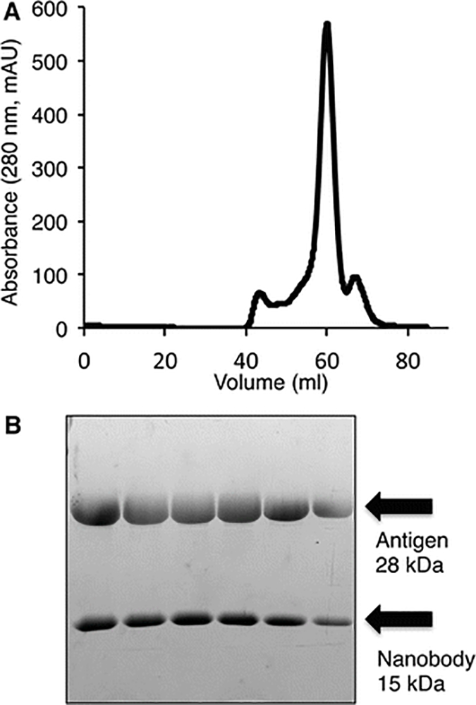
Purification of nanobody-protein antigen complex by size exclusion chromatography. (A) Chromatogram of 10 mg of nanobody-antigen complex injected onto a HiLoad 16/600 Superdex 75 pg gel filtration column. Only a single major peak elutes from the column. (B) SDS-PAGE of the major peak from purified nanobody-antigen complex.

3.4. Crystal screening and optimization

1. Concentrate the purified nanobody-antigen complex using an Amicon Ultra-4 centrifugal filter (NMWL = 10 kDa). Centrifuge the filter in a swinging bucket rotor (3,000 x g, 4 °C, 10 min). The final protein concentration should be between 10–20 mg/ml. A minimum of 100 μl of concentrated protein is required for the initial crystal screen.

2. Robotic screening is used to conduct the initial crystal screen. Prepare approximately 70 μl of nanobody-antigen complex for the preliminary screen. Centrifuge the protein sample (12,000 x g, 3 min, room temperature) to remove any precipitate.

3. Screen the nanobody-antigen complex using the PEGrx screen (Hampton Research) and the Index HT screen (Hampton Research). In general, we have had great success using these two screens for antibody crystallization. Using a Crystal Gryphon crystal robot (Art Robbin Instrument) (refer to manufacturer for operation of the robot) dispense 0.3 μl of nanobody-antigen complex with 0.3 μl of crystal screen onto a INTELLI 3-well 96 well crystallization plate.

4. Store the plate in a temperature-controlled incubator (18–20 °C) and monitor the plates for crystal formation using a stereomicroscope. Typically, the plate is monitored every 2 days for 1–2 weeks. If no crystals appear in that time frame, the plates should be kept and monitored weekly for up to 1 year. If no crystals form within a reasonable time frame, the protein complex can be re-screened (see Note 2).

5. Prepare a 24 well plate for crystal optimization by applying a layer of vacuum grease to edge of each well using a 10 ml syringe equipped a 200 μl pipette tip that has been cut to allow the viscous grease through.

6. Crystal optimizations are carried out using the hanging drop method in 24-well plates. Beginning with the initial crystal condition, design a 2D grid screen around the original condition. The variables to be adjusted are the pH of the buffer and the concentration of precipitant. On the Y-axis of the plate the pH of the buffer is adjusted in increments of 0.2, and on the X-axis the concentration of precipitant is adjusted by 2–5%. A sample optimization scheme is shown in Fig. 2.

7. Prepare 500 μl of reservoir solution by mixing water, buffer and precipitant to the bottom of each well of the 24 well plate. Mix the reservoir solution of each well in the plate using a pipette.

8. Using square plastic cover slips, pipette 1.5 μl of reservoir solution and 1.5 μl of the concentrated nanobody-antigen solution. Carefully flip the slide upside down and place it on top of well of the plate. Repeat this for the entire plate.

9. Store the plate in a temperature-controlled incubator (18–20 °C) and monitor the plates for crystal formation using a stereomicroscope.

10. Steps 6–9 can be repeated as needed until large, well-formed crystals appear. Other variable that can be modified include, varying the ratio of reservoir solution to protein (often increasing the amount of protein to reservoir volume can be beneficial), the concentration of protein, the type of buffer, the addition of small molecule additives, and varying the concentration of other components in the crystal mixture.

11. Once large crystals appear, they should be frozen for X-ray data collection. Prepare 1 ml of reservoir solution supplemented with 25 % glycerol or PEG 400 as cryoprotectant.

12. Remove the coverslip from the optimization plate that contains the desired crystal. Place the coverslip so the drop is facing up, and carefully pipette 2–3 μl of the cryoprotectant solution directly beside the drop containing the crystal.

13. Loop the crystal with a Crystalcap Cryo loop mounted on a magnetic wand, briefly dip the crystal in the cryoprotectant drop and immerse the crystal in liquid nitrogen for 30s. Never removing the crystal from the liquid nitrogen, place the crystal in a Cryocap and store the crystal on a cane.

14. Store frozen crystals in a liquid nitrogen containing dewar until ready for data collection.

Fig. 2.

Sample 2D grid crystal optimization screen carried out in a 24-well plate. The initial crystal appeared during robotic screening in the PEG Rx screen (Hampton Research). The pH of the buffer is adjusted along the X-axis of the plate, and the concentration of precipitant (Jeffamine in this case) is adjusted along the Y-axis.

3.5. X-ray structure determination and structure based epitope mapping

1. Collect X-ray data at a synchrotron. The logistics of X-ray data collection are beyond the scope of this protocol. X-ray data should be processed with appropriate software (for example Xia2, XDS or HKL2000). Typically X-ray data of the complex should be of 3 Å resolution or better to obtain a high-quality model of the binding interactions.

2. Identify suitable models for molecular replacement. Using NCBI blast, search the sequence of the nanobody and the protein antigen against the PDB subset of the database. Identify models with highest degree of sequence similarity, and download the PDB files corresponding to the models.

3. Prepare the PDB models of the nanobody and the antigen for molecular replacement. If there are additional proteins in the files, or more than one molecule in the asymmetric units of the models, delete them so that only 1 copy of the nanobody or antigen remains in the file. Remove any waters, ligands or ions from the models using Pymol.

4. Use Phaser, as implemented in the Phenix crystallography suite [12], to solve the structure of the complex by molecular replacement, using the models prepared in step 3. A TFZ score of greater than 8 indicates that the structure has been solved.

5. Refine the structure using Phenix. The initial refinement should be greater than 5 cycles, and include a rigid body refinement.

6. Using COOT, model the structure of the complex using the electron density maps calculated by Phenix in the refinement step.

7. Following modeling, refine the structure again. Continue iterative modeling and refinement steps, until the structure is acceptable (R-factors, Ramachandran plot, rmsd bonds and angles - see Note 3).

8. Once the structure is completely modeled, the antibody-antigen contacts can be mapped in an automated fashion using the webserver PDBe PISA (http://www.ebi.ac.uk/pdbe/pisa/). Upload the refined and complete structure to the webserver and examine the protein interfaces. The results will display any hydrogen bonds and electrostatic interactions that occur between the nanobody and the protein antigen. Furthermore, the results will indicate which amino acid residues are buried upon complex formation, and thus may be significant hydrophobic or van der Waal contacts. All of the contacting amino acids on the protein antigen can be considered to be the epitope, and all of the contacting residues on the nanobody constitute the paratope. Tabulate the interaction results into a table (Table I).

9. The details of the interface can be examined directly using PyMol by selecting the interfacing residues (identified in step 8), and examining the structure in detail (Fig 3).

Table I -.

Structure Based Epitope Mapping Nanobody – Antigen Interaction

Contacts		Antibody-Antigen Interface*
Nanobody	Antigen	Nanobody	Antigen
Hydrogen Bonds
S56	D199	S30, S31, E44	N46, I48, N50
S57	D199	R50, N52, G54, G55, S56, S57	K69, F70, N72
N103	D155	R100, F101, C102, N103, T104, S106,	W90, F92
Salt-Bridges			S112, E116
R100	E160		E133, S134, Y136
R100	E202		D155, S158, E160
			Q177, N178, Y80
			D199, V200, E202, F204

^*Residues in columns are not in direct contact with each other. Residues are grouped by proximity in primary sequence.

Fig 3.

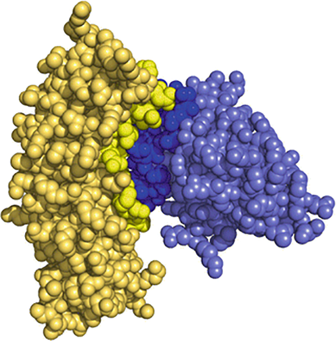
Epitope-mapping of a nanobody-protein antigen obtained through structural analysis. The interface residues between the nanobody (dark blue) and the protein antigen (yellow) are obtained using PDBe PISA server. The interfacing residues (Table I) were selected and highlighted using PyMol.

References

- 1.Martin F (2016) Antibodies as leading tools to unlock the therapeutic potential in human disease. Immunol Rev 270 (1):5–7. [DOI] [PubMed] [Google Scholar]
- 2.Strohl WR, Knight DM (2009) Discovery and development of biopharmaceuticals: current issues. Curr Opin Biotechnol 20 (6):668–672. [DOI] [PubMed] [Google Scholar]
- 3.Gebauer M, Skerra A (2009) Engineered protein scaffolds as next-generation antibody therapeutics. Curr Opin Chem Biol 13 (3):245–255. [DOI] [PubMed] [Google Scholar]
- 4.Steeland S, Vandenbroucke RE, Libert C (2016) Nanobodies as therapeutics: big opportunities for small antibodies. Drug Discov Today 21 (7):1076–1113. [DOI] [PubMed] [Google Scholar]
- 5.Liljeroos L, Malito E, Ferlenghi I, Bottomley MJ (2015) Structural and Computational Biology in the Design of Immunogenic Vaccine Antigens. J Immunol Res 2015:156241. [DOI] [PMC free article] [PubMed] [Google Scholar]
- 6.Carter JM, Loomis-Price L (2004) B cell epitope mapping using synthetic peptides. Curr Protoc Immunol Chapter 9:Unit 9 4. [DOI] [PubMed] [Google Scholar]
- 7.Bardelli M, Livoti E, Simonelli L, Pedotti M, Moraes A, Valente AP, Varani L (2015) Epitope mapping by solution NMR spectroscopy. J Mol Recognit 28 (6):393–400. [DOI] [PubMed] [Google Scholar]
- 8.Opuni KF, Al-Majdoub M, Yefremova Y, El-Kased RF, Koy C, Glocker MO (2016) Mass spectrometric epitope mapping. Mass Spectrom Rev. [DOI] [PubMed] [Google Scholar]
- 9.Walter G (1986) Production and use of antibodies against synthetic peptides. J Immunol Methods 88 (2):149–161. [DOI] [PubMed] [Google Scholar]
- 10.Muyldermans S (2013) Nanobodies: natural single-domain antibodies. Annu Rev Biochem 82:775–797. [DOI] [PubMed] [Google Scholar]
- 11.Arbabi-Ghahroudi M, To R, Gaudette N, Hirama T, Ding W, MacKenzie R, Tanha J (2009) Aggregation-resistant VHs selected by in vitro evolution tend to have disulfide-bonded loops and acidic isoelectric points. Protein Eng Des Sel 22 (2):59–66. [DOI] [PubMed] [Google Scholar]
- 12.Adams PD, Afonine PV, Bunkoczi G, Chen VB, Davis IW, Echols N, Headd JJ, Hung LW, Kapral GJ, Grosse-Kunstleve RW, McCoy AJ, Moriarty NW, Oeffner R, Read RJ, Richardson DC, Richardson JS, Terwilliger TC, Zwart PH (2010) PHENIX: a comprehensive Python-based system for macromolecular structure solution. Acta Crystallogr D Biol Crystallogr 66 (Pt 2):213–221. [DOI] [PMC free article] [PubMed] [Google Scholar]
- 13.Emsley P, Lohkamp B, Scott WG, Cowtan K (2010) Features and development of Coot. Acta Crystallogr D Biol Crystallogr 66 (Pt 4):486–501. [DOI] [PMC free article] [PubMed] [Google Scholar]