Soft-Split Random Forest for Anatomy Labeling

Abstract

Random Forest (RF) has been widely used in the learning-based labeling. In RF, each sample is directed from the root to each leaf based on the decisions made in the interior nodes, also called splitting nodes. The splitting nodes assign a testing sample to either left or right child based on the learned splitting function. The final prediction is determined as the average of label probability distributions stored in all arrived leaf nodes. For ambiguous testing samples, which often lie near the splitting boundaries, the conventional splitting function, also referred to as hard split function, tends to make wrong assignments, hence leading to wrong predictions. To overcome this limitation, we propose a novel soft-split random forest (SSRF) framework to improve the reliability of node splitting and finally the accuracy of classification. Specifically, a soft split function is employed to assign a testing sample into both left and right child nodes with their certain probabilities, which can effectively reduce influence of the wrong node assignment on the prediction accuracy. As a result, each testing sample can arrive at multiple leaf nodes, and their respective results can be fused to obtain the final prediction according to the weights accumulated along the path from the root node to each leaf node. Besides, considering the importance of context information, we also adopt a Haar-features based context model to iteratively refine the classification map. We have comprehensively evaluated our method on two public datasets, respectively, for labeling hippocampus in MR images and also labeling three organs in Head & Neck CT images. Compared with the hard-split RF (HSRF), our method achieved a notable improvement in labeling accuracy.

1 Introduction

Many anatomy labeling methods have been proposed recently. These methods can be roughly categorized into two classes: 1) multi-atlas based and 2) learning-based methods. In the multi-atlas based methods, a set of already-labeled images, namely atlases, are used to guide the labeling of new target image [1]. Specifically, given a new target image, multiple atlas images are first registered onto this target image, and then the estimated deformation fields are applied to transform the corresponding label maps of atlases to the target image. Finally, all warped atlas label maps are fused for labeling the target image. Specially, in the label fusion step, patch-based similarity is often used as weight to propagate the neighboring atlas labels to the target image, for potentially overcoming errors from the registration. The limitation of multi-atlas based methods is that 1) the labeling accuracy highly depends on registration between atlas and target images; 2) the patch similarity is often handcrafted based on the predefined features (e.g., image intensity), which might not be effective for labeling all types of anatomical structures, thus potentially limiting the labeling accuracy.

On the other hand, learning-based labeling methods have attracted much attention recently. In the learning-based methods, a strong classifier, such as Adaboost [2], random forests [3] and artificial neural networks [4], is often used to classifying whether a voxel belongs to the interested anatomical structure, based on the local appearance features. In the testing stage, the learned classifiers are applied to voxel-wisely classify the whole target image. These learning-based labeling methods can identify the discriminative features specific to each anatomical structure and make full use of appearance information for anatomy labeling. For example, Zikic et al. [5] developed so-called atlas forest to learn a classification forest for each atlas. Tu et al. [6] adopted the probabilistic boosting tree (PBT) for labeling the MR brain images with Haar features and texture features. Also, Kim et al. [7] utilized Adaboost algorithm to train classifiers in multiple atlas image spaces. Then, the final segmentation of a target image is achieved by averaging the labeling results from all classifiers. In addition to just using local appearance information, many researches have shown that the context information is also very useful in identifying an object from a complex scene. In the field of anatomy labeling, many learning-based methods combined appearance with context features to improve the labeling accuracy. For example, Zikic et al. [5] constructed a population mean atlas to provide the rough context information for the target image. Tu et al. [6] proposed an auto-context model (ACM) to extract the context information embedded in the tentative labeling map of the target image for iterative refinement of labeling results. Kim et al. [7] extracted the context information from an initial labeling probability map of the target image, obtained by using the multi-atlas based method. Compared to the multi-atlas based methods, the learning-based methods can easily learn discriminative features and further utilize context information to improve the labeling performance.

Our method belongs to the learning-based labeling methods. Specifically, we use random forest as classifier for voxel-wise labeling. The major contribution of our paper is proposing a novel variant of random forest, namely soft-split random forest (SSRF), which improves the performance of the conventional RF in anatomical labeling. In the conventional RF, a testing sample follows one path from the root to leaf, based on the decisions made at each splitting node. For the ambiguous testing samples, which often locate near the splitting boundaries, they can arrive at a wrong leaf node due to the wrong assignment made in any of the splitting nodes. To overcome this problem, we propose a “soft split” strategy to handle this problem. Specifically, in each split, we take a probabilistic view and allow each sample to go both left and right nodes with their certain probabilities, which are determined according to the distance of this sample to the splitting decision boundary. Finally, the probability for each leaf is the multiplication of all probabilities along the path, and the prediction of a sample is the weighted average over all non-zero leaf nodes. By using this strategy, we can relieve the problem caused by the mis-assignment in any of the splitting nodes. Experimental results show significant improvement by using SSRF, compared to the conventional RF. Besides, to further refine the labeling result, Haar-features based context model (HCM) is proposed to iteratively construct a sequence of classification forests by updating the context features from the newly-estimated label maps for training. Validated on two public datasets, ADNI and Head & Neck datasets, our proposed method consistently outperforms the conventional RF (using the hard split function).

2 Random Forest

Random Forest (RF) is an ensemble learner, which consists of multiple decision trees. Each tree is independently trained in a randomized fashion. Since the RF classifier is able to handle a high-dimension feature space efficiently and is inherently multi-class, it has recently gained popularity on anatomy labeling. As similar to the common learning techniques, random forest consists of training and testing stages.

RF Training

Given a set of training data D = {(h_i, l_i)|i = 1, …, N}, where h_i and l_i are the feature vector and class label of the i-th training sample, RF aims to learn a non-linear mapping from the feature vector h of a sample to the corresponding class label l by constructing multiple decision trees. In RF classification, each decision tree is independently trained based on one subset of samples randomly extracted from the training set D. In terms of the tree structure, a decision tree consists of two types of nodes, namely split nodes and leaf nodes. Each split node links two child nodes (left and right child nodes). In order to build a decision tree for classification, a split function is learned at each split node, which optimally splits the samples into two child nodes. A standard split function (decision stump function) is defined as follows:

$$f\left(\mathbf{h}|j,\tau \right)=\{\begin{array}{l}0,h\left(j\right)\le \tau \hfill \\ 1,h\left(j\right)>\tau \hfill \end{array}$$ (1)

where j is the element index of h, h(j) is the j-th feature of h, and τ is a threshold. If h(j) ≤ τ, f(h|j, τ) is set zero, indicating that the sample h is assigned to left-child node; otherwise, if f(h|j, τ) is one, the sample h is assigned to right-child node. To determine the optimal combination of feature and threshold, a random sub-set of features and the corresponding thresholds are sampled and tested. The one that offers the maximum entropy reduction is regarded as the optimal pair for this split function. After learning the split function, the samples are split and passed to two child nodes for recursive splitting. The training of a decision tree starts with finding the optimal split at the root node, and then recursively proceeds on child nodes until either the maximum tree depth is reached or the number of training samples is too small to split. Finally, the leaf node stores the class label distribution p(l) of all training samples falling into this leaf node.

RF Testing

For a new testing sample, RF pushes it through each learned decision tree, starting at the root node. At each split node, the testing sample is assigned to one of child nodes by applying the corresponding decision stump function. If the function response is zero, the testing sample is assigned to the left child node; if the function response is one, it is assigned to the right child node. When the testing sample reaches a leaf node, the class label distribution p(l) stored in that leaf node is used as the output of the decision tree and assigned as the probability of the testing sample belonging to class label l. For the entire forest, the final probability $\overline{p}\left(l\right)$ of the testing sample assigned to class label l is the average of outputs from all decision trees, i.e. $\overline{p}\left(l\right)=\frac{1}{T}{\displaystyle {\sum }_{l=1}^{T}p\left(l\right)}$, where T is the number of decision trees.

3 Proposed Method

3.1 Soft-Split Random Forest

In the testing stage, the conventional random forest makes “hard split” (i.e., either left or right) at each split node and thus assigns each sample with only one path from the root to a leaf node. This splitting strategy is effective when there exist a clear boundary among samples of different class labels. However, there may exist ambiguous samples, which lie near (or even lie on) splitting boundaries (Fig. 1(a)), which could lead to wrong assignment. Specifically, training samples may highly overlap in the feature space (Fig. 1(b)), which makes it difficult to find a clear separation/split. That is, there will be many “hard-to-split” samples close to the splitting hyper-plane, which are ambiguous in some sense. For those samples, even though they locate on one side of the hyper-plane, they are also likely belonging to the other side due to small noise. The conventional way of hard split tends to ignore this fact, and may misclassify sample to wrong side, thus leading to inaccurate prediction.

Fig. 1.

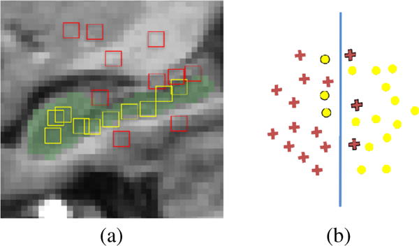
Feature space distribution of voxels inside and outside hippocampus. Red and yellow boxes in (a) represent local patches of voxels outside and inside the hippocampus, respectively. Red crosses and yellow circles in (b) represent feature distributions of voxels outside and inside the hippocampus, respectively. Blue vertical line in (b) denotes a splitting decision boundary.

To solve this problem, we propose to use “soft split” strategy applied in the testing stage. The basic idea of soft split is that, when a new sample comes to a split node, instead of classifying it into only one child node in each split, we take a probabilistic view and allow each sample go to both left and right nodes with certain probabilities, which are determined by the distance of this sample to the learned splitting decision boundary. Finally, the probability of each leaf is the multiplication of all probabilities along the path from the root to the leaf, and the label probability of a testing sample is the weighted average of all leaf nodes of all trees visited with non-zero probability.

Specifically, in the testing stage of RF, for each split node, we define a soft split function based on the distance of the testing sample to the learned splitting decision boundary. Mathematically, the soft split function is defined as follows:

$$f_S\left({\mathbf{h}}_t|j_0,{\tau }_0\right)=\frac{1}{1+e^{-\sigma d}},d=\{\begin{array}{l}\frac{h_t\left(j_0\right)-{\tau }_0}{r_{\mathit{max}}-{\tau }_0}{h}_t\left(j\right)\ge {\tau }_0\hfill \\ \frac{h_t\left(j_0\right)-{\tau }_0}{{\tau }_0-r_{\mathit{min}}}{h}_t\left(j\right)\le {\tau }_0\hfill \end{array}$$ (2)

where h_t is the feature vector of the testing sample, j₀ and τ₀ are the optimal feature index and threshold of the hard split function learned in the training stage, r_min and r_max are the minimum and maximum feature responses of training samples arrived in this split node, respectively, and σ is the tuning parameter that controls the slop of the function. To avoid the problem caused by different feature scales, the distance d is normalized to [0,1] by using r_min and r_max. Based on the soft split function, we use p_R = f_S and p_L = 1 − f_S for indicating the probabilities of the testing sample assigned to the right child node and the left child node, respectively. It can be clearly seen from f_S that when h_t(j) ≫ τ₀, p_R → 1 and when h_t(j) ≪ τ₀, p_R → 0; e.g., the larger distance between feature response h_t(j₀) and the boundary τ₀ is, the more extreme the probabilities are. To improve the testing, when the feature response h_t(j₀) is far from the boundaryτ₀, the soft split function becomes hard split, and the sample is assigned to either left or right child node as follows:

$$f_S^{\prime }=\{\begin{array}{l}0f_S<c\hfill \\ f_{S}c\le f_S\le 1-c\hfill \\ 1f_S>1-c\hfill \end{array}$$ (3)

where c ∈ [0,0.5] is the cutting parameter.

Thus, using the soft split, a new sample will be split into both left and right nodes at each split node with certain probabilities. Finally, for each leaf node, its weight is computed as the multiplication of all probabilities along the path from the root node to itself. The estimated label probability of this new sample is weighted average of label probabilities of all leaf nodes across all different trees.

3.2 Haar-Features Based Context Model (HCM)

In the section, we present a Haar-features based context model (HCM) to iteratively improve the labeling accuracy by using both low-level appearance features (computed from the target image) and high-level context features (computed from tentative labeling probability maps of the target image). Specifically, at each iteration, random forest outputs a tentative labeling probability map of the target image, from which we can compute Haar-like features. These features are called context features and can be used together with the intensity features to refine the labeling results. In the following paragraphs, we detail the training and testing stages of our HCM.

Training

In the initial iteration, we first use the simple multi-atlas based majority voting to initialize the labeling probability maps of the training images. Specifically, for each training image, we linearly align all other images onto this image and then adopt the majority voting to obtain an initial labeling map by propagating labels from all aligned images to this image. In the second iteration, for each training voxel x in the training image, we extract Haar-like features from both training image and the initial labeling probability maps. The Haar-like features extracted from training image are called intensity features, and those extracted from probability maps are called context features. They can be combined as input features to train next random forest classifier. During the training of each split node, the minimum and maximum feature responses (r_min and r_max) are saved, in order to normalize the sample-to-boundary distance for the testing samples (Eq. 2). After the current RF classifier is trained, we can apply it to each training image for estimating the new labeling probability maps by combining local appearance and context information. Since the new labeling probability maps are often better than those obtained by majority voting, as shown in Fig. 2, we can use these new maps to replace those obtained by majority voting and compute the new context features. Once the context features have been updated, a new random forest classifier can be learned. This procedure is iterated until we obtain O sets of RF classifiers, each set containing one random forest classifier for each anatomical structure.

Fig. 2.

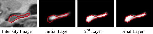
The labeling probability map of hippocampus at each iterative layer of HCM. Red contours denote the ground-truth boundary of hippocampus.

Testing

Given a new testing image, the labeling probability of each voxel is iteratively updated similarly as done in the training stage. Specifically, all the training images (atlases) are first linearly aligned onto the testing image, and majority voting is further used to fuse the label maps of all aligned atlases to initialize the probability map of the testing image. Then, Haar-like features are extracted from both testing image and the estimated probability map to serve as intensity and context features, respectively. Based on both features, with the learned RF, we can obtain new labeling probability maps, which can be fed into the next learned RF to further refine the labeling probability maps. This iterative procedure continues until all learned RF classifiers have been applied. Fig. 2 demonstrates this process of labeling hippocampus on a typical target image.

4 Experiments

In this section, we perform experimental validation of our proposed method on the ADNI¹ dataset and the Head & Neck² dataset for evaluating its performance. In ADNI dataset, we apply our method to segment the hippocampus from MRI images. In Head & Neck dataset, we apply our method to segment parotid glands and brain stem from CT images. To demonstrate the superiority of soft-split over hard-split RF, we compare our method to the hard-split RF without (HSRF) and with HCM (HSRF+HCM), respectively. To quantitatively evaluate the labeling accuracy, we use the Dice Similarity Coefficient (DSC) to measure the overlap degree between automatic and manual labeling results. In the experiments, we use five-fold cross-validation to evaluate the performance of our method, as well as the comparison methods.

Parameters

In the training stage, we train 20 trees for each RF. The maximum tree depth is set to 20, and the minimum number of samples in each leaf node is set to 4. In the training of each tree node, 1000 random Haar-like features are extracted from intensity image, and 100 random Haar-like features are extracted from the labeling probability map. σ and c in the soft-split random forest (SSRF) are set to 0.1 and 0.1, respectively.

ADNI Dataset

The ADNI dataset contains the segmentations of the left and right hippocampi (LH and RH) of brain MRIs, which have been manually labeled by expert. The size of each MR image is 256 × 256 × 256. We randomly selected 64 subjects to evaluate both performances of our method and the comparison methods. The selected subset of ADNI includes 16 normal control (NC), 32 MCI (Mild Cognitive Impairment) subjects, and 16 AD (Alzheimer Disease) subjects. The middle columns of Table 1 list the results for the labeling of left and right hippocampi. We can see that soft-split random forest improves over the hard-split random forest. With the inclusion of Haar-features based context information, the performance is further boosted. Fig. 3 demonstrates a qualitative comparison.

Table 1.

The mean and standard deviation of DSC and (%) by HSRF, HSRF+HCM, SSRF, and SSRF+HCM on ADNI and Head & Neck datasets, respectively.

Method	ADNI		Head & Neck
	LH	RH	LP	RP	BS
HSRF	82.5±4.1	81.3±4.1	77.0±6.8	78.8±5.0	83.7±4.6
HSRF+HCM	85.5±3.2	85.2±3.5	80.5±7.0	81.4±5.1	84.8±4.7
SSRF	83.9±3.5	83.8±3.2	80.4±6.7	81.7±4.7	86.1±4.3
SSRF+HCM	86.9±2.6	86.6±3.1	81.3±6.8	82.1±5.2	87.1±4.3

Fig. 3.

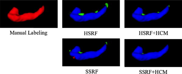
Qualitative comparison of the labeling results of hippocampus for one subject using 4 different methods (red: manual labeling result; green: automated labeling results; blue: overlap between manual and automated labeling results).

Head & Neck Dataset

The Head & Neck dataset consists of 40 CT images. Each image contains manually labeled left and right parotid glands (LP and RP), and brain stem (BS). The spatial resolution of 40 CT images ranges over [0.76 − 2.34] × [0.76 − 2.34] × [1.25 − 3] mm. The right columns of Table 1 show the labeling results for the left and right parotid glands, and brain stem, which also indicates the advantages of our proposed soft-splitting and HCM. Fig. 4 provides a qualitative comparison. To provide some comparisons, we cite recent results from [8]. In [8], the authors proposed a segmentation method based on multiple atlases, statistical appearance models and geodesic active contours (MABSInShape), which obtains average DSC 81% for LP, 84% for RP, and 86% for BS. It is worth noting that this method is evaluated on a subset of our dataset with only 18 high-resolution CT images, while we use 40 CT images containing both low- and high- resolution CT Images. Specifically, for high-resolution CT image set, SSRF and SSRF+HCM methods respectively obtain the average DSC 82% and 83% for LP, 85% and 86% for RP, and 88% and 89% for BS. By comparing our methods with MABSInShape, our methods also obtain better results.

Fig. 4.

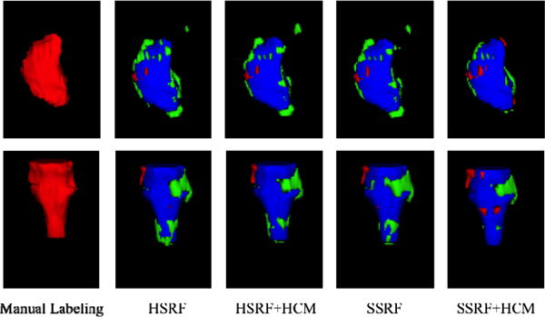
Qualitative comparison of labeling results of LP (top) and BS (bottom) for one subject using 4 different methods (red: manual labeling results; green: automated labeling results; blue: overlap between manual and automated labeling results).

5 Conclusion

In this paper, we propose a soft-split random forest (SSRF) to effectively improve the reliability of the conventional random forest. Besides, the Haar-features based context model (HCM) is also proposed to improve the labeling performance by utilizing the context information of the target image. Specifically, we use Haar-like features to iteratively extract context information from the tentatively-estimated labeling probability maps of the target image. Our method shows more accurate labeling results than the conventional RF, on both ADNI and Head & Neck datasets.

References

- 1.Wang H, et al. Multi-atlas segmentation with joint label fusion. IEEE Transactions on Pattern Analysis and Machine Intelligence. 2013;35(3):611–623. doi: 10.1109/TPAMI.2012.143. [DOI] [PMC free article] [PubMed] [Google Scholar]
- 2.Freund Y, et al. A decision-theoretic generalization of on-line learning and an application to boosting. In: Vitányi PM, editor. EuroCOLT 1995 LNCS. Vol. 904. Springer; Heidelberg: 1995. [Google Scholar]
- 3.Breiman L. Random forests. Machine learning. 2001;45(1):5–32. [Google Scholar]
- 4.Magnotta VA, et al. Measurement of Brain Structures with Artificial Neural Networks: Two-and Three-dimensional Applications 1. Radiology. 1999;211(3):781–790. doi: 10.1148/radiology.211.3.r99ma07781. [DOI] [PubMed] [Google Scholar]
- 5.Zikic D, Glocker B, Criminisi A. Atlas encoding by randomized forests for efficient label propagation. In: Mori K, Sakuma I, Sato Y, Barillot C, Navab N, editors. MICCAI 2013, Part III. Vol. 8151. Springer; Heidelberg: 2013. pp. 66–73. (LNCS). [DOI] [PubMed] [Google Scholar]
- 6.Tu Z, et al. Auto-context and its application to high-level vision tasks and 3d brain image segmentation. IEEE Transactions on Pattern Analysis and Machine Intelligence. 2010;32(10):1744–1757. doi: 10.1109/TPAMI.2009.186. [DOI] [PubMed] [Google Scholar]
- 7.Kim M, et al. Automatic hippocampus segmentation of 7.0 Tesla MR images by combining multiple atlases and auto-context models. NeuroImage. 2013;83:335–345. doi: 10.1016/j.neuroimage.2013.06.006. [DOI] [PMC free article] [PubMed] [Google Scholar]
- 8.Fritscher KD, et al. Automatic segmentation of head and neck CT images for radiotherapy treatment planning using multiple atlases, statistical appearance models, and geodesic active contours. Medical Physics. 2014;41(5) doi: 10.1118/1.4871623. [DOI] [PMC free article] [PubMed] [Google Scholar]