Abstract
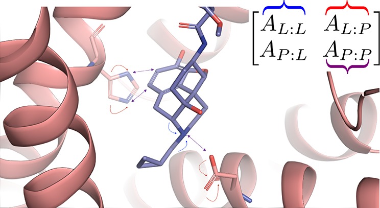
The arc of drug discovery entails a multiparameter optimization problem spanning vast length scales. The key parameters range from solubility (angstroms) to protein–ligand binding (nanometers) to in vivo toxicity (meters). Through feature learning—instead of feature engineering—deep neural networks promise to outperform both traditional physics-based and knowledge-based machine learning models for predicting molecular properties pertinent to drug discovery. To this end, we present the PotentialNet family of graph convolutions. These models are specifically designed for and achieve state-of-the-art performance for protein–ligand binding affinity. We further validate these deep neural networks by setting new standards of performance in several ligand-based tasks. In parallel, we introduce a new metric, the Regression Enrichment Factor EFχ(R), to measure the early enrichment of computational models for chemical data. Finally, we introduce a cross-validation strategy based on structural homology clustering that can more accurately measure model generalizability, which crucially distinguishes the aims of machine learning for drug discovery from standard machine learning tasks.
Short abstract
We introduce PotentialNet, a neural network designed to share information among atoms in the same system, and investigate its performance in predicting protein−ligand binding and molecular properties.
I. Introduction
Most FDA-approved drugs are small organic molecules that elicit a therapeutic response by binding to a target biological macromolecule. Once bound, small molecule ligands either inhibit the binding of other ligands or allosterically adjust the target’s conformational ensemble. Binding is thus crucial to any behavior of a therapeutic ligand. To maximize a molecule’s therapeutic effect, its affinity—or binding free energy (ΔG)—for the desired targets must be maximized, while simultaneously minimizing its affinity for other macromolecules. Historically, scientists have used both cheminformatic and structure-based approaches to model ligands and their targets, and most machine learning (ML) approaches use domain-expertise-driven features.
More recently, deep neural networks (DNNs) have been translated to the molecular sciences. Training most conventional DNN architectures requires vast amounts of data: for example, ImageNet1 currently contains over 14 000 000 labeled images. In contrast, the largest publicly available data sets for the properties of druglike molecules include PDBBind 2017,2 with a little over 4000 samples of protein–ligand cocrystal structures and associated binding affinity values; Tox21 with nearly 10 000 small molecules and associated toxicity end points; QM8 with around 22 000 small molecules and associated electronic properties; and ESOL with a little over 1000 small molecules and associated solubility values.3 This scarcity of high-quality scientific data necessitates innovative neural architectures for molecular machine learning.
Successful DNNs often exploit relevant structure in data, such as pixel proximity in images. Predicting protein–ligand binding affinity seems to resemble computer vision problems. Just as neighboring pixels connote closeness between physical objects, a binding pocket could be divided into a voxel grid. Here, neighboring voxels denote neighboring atoms and blocks of empty space. Unfortunately, this 3D convolutional approach has several potential drawbacks. First, inputs and hidden weights require much more memory in three dimensions. Second, since the parameters grow exponentially with the number of dimensions, the model suffers from the “curse of dimensionality”:4 while image processing may entail a square 32 filter, the corresponding filter for volumetric molecule processing has 33 parameters.
In contrast, graph convolutions use fewer parameters by exploiting molecular structure and symmetry. Consider a carbon bonded to four other atoms. A 3D convolutional neural network (CNN) would need several different filters to accommodate the subgroup’s symmetrically equivalent orientations. However, a graph convolution as described in refs (5−8) is symmetric to permutations and relative location of each of the four neighbors, thereby significantly reducing the number of model parameters. The use of graph convolutional approaches to learn molecular properties is reminiscent of the familiar canon of chemoinformatics algorithms such as Morgan fingerprints,9 SMILES strings,10 and the Ullman algorithm for substructure search,11 all of which enrich chemical descriptions by propagating information about neighboring atoms.
In this paper, we first review a subset of DNN architectures applicable to protein–ligand interaction. Through the mathematical frameworks above, we contextualize our presentation of new models that generalize a graph convolution to include both intramolecular interactions and noncovalent interactions between different molecules. We describe a staged gated graph neural network, which distinguishes the derivation of differentiable bonded atom types from the propagation of information between different molecules. Finally, we address a potential shortcoming of the standard benchmark in this space—namely, treating the PDBBind 2007 core set as a fixed test set—by choosing a cross-validation strategy that more closely resembles the reality of drug discovery. Though more challenging, this benchmark may better reflect a given model’s generalization capacity.
II. Neural Network Architectures
First, we briefly review a subset of DNN architectures applicable to protein–ligand interaction to motivate the new models we present and test at the end of the paper.
II.A. Ligand-Based Scoring Models
II.A.1. Fully Connected Neural Networks
The qualitatively simplest models for affinity prediction and related tasks incorporate only features of ligands and ignore the macromolecular target(s). Such a model could entail a fully connected neural network (FCNN), in which each molecule is represented by a flat vector x containing f0 features. Then, these features are updated through “hidden” layers h by applying nonlinear activation functions.
The training data for such a network consists of a set of N molecules, each represented by a vector of length f0, which have a one-to-one correspondence with a set of N affinity labels. Domain-expertise-driven flat vector features might include integer counts of different types of predetermined functional groups (e.g., carboxylic acids, aromatic rings), polar or nonpolar atoms, and other ligand-based features. Cheminformatic featurizations include extended circular fingerprints (ECFP)12 and ROCS.13,14
II.A.2. Graph Convolutional Neural Networks
In convolutional neural networks (CNNs), each layer convolves the previous layer’s feature map with linear kernels followed by elementwise nonlinearities, producing new features of higher complexity that combine information from neighboring pixels.15 A graph convolutional neural network (GCNN) analogously exploits the inherent structure of data.16 We can represent a given graph that contains N nodes, fin features per node, and a single edge type, as consisting of node features x and symmetric adjacency matrix A, which designates whether a pair of nodes belong to each other’s neighbor sets N. Consider the molecule propanamide (Figure 1). For the carbonyl carbon, the relevant row of the feature matrix x might be [1, 0, 0] to represent its element, and the corresponding row of the adjacency matrix A might be [0, 1, 0, 1, 1] to indicate its bonds to three neighbor atoms.
Figure 1.
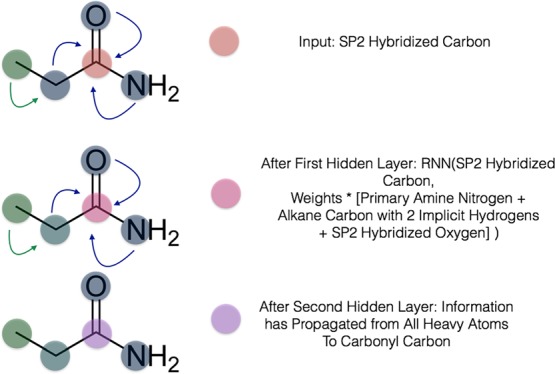
Visual depiction of the gated graph neural network with atoms as nodes and bonds as edges. The small molecule propanamide is chosen to illustrate the propagation of information among the different update layers of the network.
A graph convolution update, as summarized in ref (8), entails applying a function at each node that takes the node and its neighbors as input and outputs a new set of features for each node. It can be written as
 |
1 |
where hi(t) represents the node features of node i at hidden layer t, N(vi) represents the neighbors of node i, and U(t) and m(t) are the update and message functions, respectively, at hidden layer t. When there are multiple edge types, we must define multiple message functions, m(t,e), which is the message function at layer t for edge type e ∈ [1, ···, Net].
Our models are primarily inspired by the gated graph neural networks (GGNNs).7 At all layers, the update function is the familiar gated recurrent unit (GRU). Message functions are simple linear operations that are different for each edge type but also the same across layers:
| 2 |
where A(e) is the adjacency matrix, and W(e) the weight matrix, respectively, for edge type e.
Unlike conventional FCNNs, which learn nonlinear combinations of the input hand-crafted features, the update described in eq 2 learns nonlinear combinations of more basic features of a given atom with the features of its immediate neighbors. Information propagates through increasingly distant atoms with each graph convolution, and the GRU enables information to be added selectively. Ultimately, the GGNN contains and leverages both per-node features via the feature matrix x and structural information via the adjacency matrix A. In both classification and regression settings, GCNNs terminate in a “graph gather” step that sums over the rows of the final embeddings and is invariant to node ordering. The subsequent FCNNs produce output of desired size (fout). This completes the starting point for the graph convolutional update used in this paper:
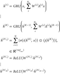 |
3 |
II.A.3. Generalization to Multitask Settings
Predicting affinity
for multiple targets by GCNN can be implemented
by training either different models for each target or by training
a single multitask network. The latter setting has a last weight matrix  , where T denotes the number
of targets in the data set. The corresponding multitask loss function
would be the average binary cross-entropy loss across the targets
 |
4 |
II.B. Structure-Based Scoring Models
Since the advent of biomolecular crystallography by Perutz et al.,17 the drug discovery community has sought to leverage structural information about the target in addition to the ligand. Numerous physics-based approaches have attempted to realize this, including molecular docking,18−21 free energy perturbation,22 and quantum mechanics/molecular mechanics (QM/MM),23 among others. More recent approaches include RF-Score,24,25 NN-Score,26 Grid Featurizer,3 three-dimensional CNN approaches,27,28 and Atomic Convolutional Neural Networks.29
II.B.1. PotentialNet Architectures for Molecular Property Prediction
To motivate architectures for more principled
DNN predictors, we invoke the following notation and framework. First,
we introduce the distance matrix  , whose entries Rij denote the distance between atomi and atomj. Thus
far, the concept
of adjacency, as encoded in a symmetric matrix A,
has been restricted to chemical bonds. However, adjacency can also
encompass a wider range of neighbor types to include noncovalent interactions
(e.g., π–π stacking, hydrogen bonds, hydrophobic
contact). Adjacency need not require domain expertise: pairwise distances
below a threshold value can also be used. Regardless of a particular
scheme, we see how the distance matrix R motivates
the construction of an expanded version of A. In
this framework, A becomes a tensor of shape N × N × Net, where Net represents the number
of edge types.
If we order the rows by the membership of atomi to either the protein or ligand, we can view both A and R as block matrices, where the diagonal blocks are self-edges (i.e., bonds and noncovalent interactions) from one ligand atom to another ligand atom or from one protein atom to another protein atom, whereas off-diagonal block matrices encode edges from the protein to the ligand and from ligand to protein. For illustration purposes, we choose the special case where there is only one edge type, Net = 1:
 |
5 |
where Aij is 1 for neighbors
and 0 otherwise, and  . Within this framework,
we can mathematically
express a spatial graph convolution—a graph
convolution based on notions of adjacency predicated on Euclidean
distance—as a generalization of the GGNN characterized by the
update, eq 2.
In addition to edge type generalization, we introduce nonlinearity in the message portion of the graph convolutional layer:
| 6 |
where NN(e) is a neural network for each edge type e and N(e)(hi) denotes the neighbors of edge type e for atom/node i.
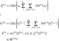
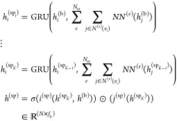
Finally, we generalize the concept of a layer to the notion of a stage that can span several layers of a given type. The staged PotentialNet consists of three main steps: (1) covalent-only propagation, (2) dual noncovalent and covalent propagation, and (3) ligand-based graph gather (see Figure 2). Stage 1, covalent propagation, entails only the first slice of the adjacency matrix, A(1), which contains a 1 at entry (i, j) if there is a bond between (atomi, atomj) and a 0 otherwise. Intuitively, stage 1 computes a new set of vector-valued atom types hi(b) for each of the N atoms in the system based on their local networks of bonded atoms (see Figure 3). Subsequently, stage 2 entails propagation based on both the full adjacency tensor A which begins with the vector-valued atom types hi computed in eq 1. While stage 1 computes new bond-based “atom types” for both amino acid and ligand atoms, stage 2 passes both bond and spatial information between the atoms. For instance, if stage 1 distinguishes an amide carbonyl oxygen from a ketone carbonyl oxygen, stage 2 might communicate in the first layer that that carbonyl oxygen is also within 3 Å of a hydrogen bond donor (see Figure 4). Finally, in stage 3 a graph gather is performed solely on the ligand atoms. The ligand-only graph gather is made computationally straightforward by the block matrix formulation described in eq 5.
 |
7 |
 |
8 |
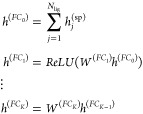 |
9 |
where i(b), j(b), i(sp), j(sp) are (b)ond and (sp)atial neural networks, and hj(sp) denotes the feature map for the jth atom at the end of stage 2.
Figure 2.
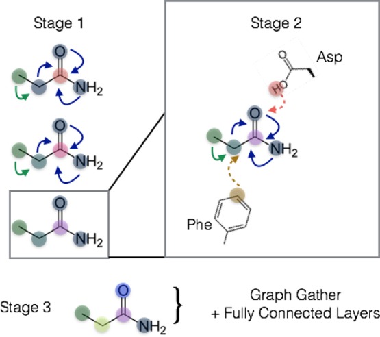
Visual depiction of multistaged spatial gated graph neural network. Stage 1 entails graph convolutions over only bonds, which derives new node (atom) feature maps roughly analogous to differentiable atom types in more traditional forms of molecular modeling. Stage 2 entails both bond-based and spatial distance-based propagation of information. In the final stage, a graph gather operation is conducted over the ligand atoms, whose feature maps are derived from bonded ligand information and spatial proximity to protein atoms.
Figure 3.
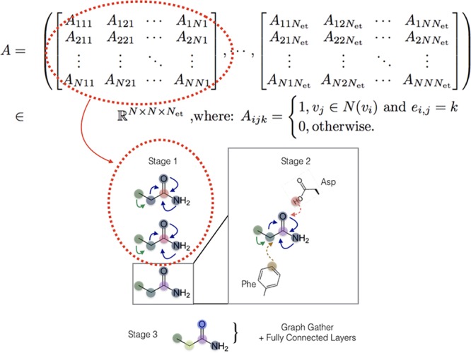
PotentialNet stage 1 exploits only covalent or bonded interaction edge types encoded in the first slices of the last dimension of the adjacency tensor A.
Figure 4.
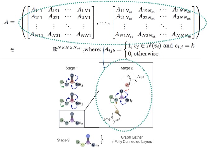
PotentialNet stage 2 exploits both bonded and nonbonded interaction edge types spanning the entirety of the last dimension of the adjacency tensor A.
A theoretically attractive concept in eq 7 is that atom types—the 1 × fb per-atom feature maps—are derived from the same initial features for both ligand and protein atoms. In contrast to molecular dynamics force fields,30 which—for historical reasons—have distinct force fields for ligands and for proteins which then must interoperate (often poorly) in simulation, our approach derives the physicochemical properties of biomolecular interactions from a unified framework.
To further illustrate this, PotentialNet stage 1 and stage 2 exploit different subsets of the full adjacency tensor A.
III. Measuring Early Enrichment in Regression Settings for Virtual Screening
Traditional metrics of predictor performance suffer from general problems and drug discovery-specific issues. For regressors, both R2—the “coefficient of determination”—and the root-mean-square error (RMSE) are susceptible to single data point outliers. The RMSE for both classifiers and regressors account for neither the training data distribution nor the null model performance. The area under the receiver operating characteristic curve (AUC)31 does correct this deficiency in RMSE for classifiers. However, all aforementioned metrics are global statistics that equally weight all data points. This property is particularly undesirable in drug discovery, which is most interested in predicting the tails of a distribution: while model predictions are made against an entire library containing millions of molecules, one will only purchase or synthesize the top scoring molecules. In response, the cheminformatics community has adopted the concept of early enrichment. Methods like BEDROC32 and LogAUC33 weight the importance of the model’s highest performers more heavily.
III.A. Proposed Metric: EFχ(R)
At present, this progress in early enrichment measurement has been limited to classification and has yet to include regression. Therefore, we propose a new metric for early enrichment in regression, the Regression Enrichment Factor, EFχ(R), analogous to EFχ. For a given target
| 10 |
in which yi values, the experimental (observed) measurement for sample i, are ranked in descending order according to ŷi, the model (predicted) measurement for sample i. In other words, we compute the average z-Score for the observed values of the top χ% scoring samples. We prefer this approach to computing, for example, 1/χ·N∑iχ·N(yi – y̅), which has units that are the same as yi (i.e., log(Ki) values). Unfortunately, this unnormalized approach depends on the distribution in the data set. For instance, in a distribution of log(Ki) measurements, if the maximum deviation from the mean is 1.0, the best a model can possibly perform would be to achieve an EFχ of 1.0.
We normalize through division by σ(y), the standard deviation of the data. This allows comparison of model performance across data sets with a common unit of measurement but different variances in those measurements. The upper bound is therefore equal to the right-hand side of eq 10, where the indexed set of molecules i constitutes the subset of the χ·N most experimentally active molecules. This value is dependent on both the distribution of the training data as well as the value χ. The EFχ(R) is an average over χ·N z-scores, which themselves are real numbers of standard deviations away from the mean experimental activity.34
IV. Results
IV.A. Cross-Validation Strategies
It is well-known that the performance of DNN algorithms is highly sensitive to chosen hyperparameters. Such sensitivity underscores the criticality of rigorous cross-validation.35,36 Several recent papers, including works that claim specifically to improve binding affinity prediction on the PDBBind data set,37,38 engage in the practice of searching hyperparameters directly on the test set. Compounding this problem is a fundamental deficiency of the main cross-validation procedure used in this subfield that is discussed below.
While there are newer iterations of the PDBBind data set, e.g., ref (2), we choose to evaluate performance on PDBBind 200739,40 to compare performance of our proposed architectures to previous methods. In previous works, the PDBBind 2007 data set was split by (1) beginning with the “refined” set comprising 1300 protein–ligand cocrystal structures and associated binding free energy; (2) removing the “core” set comprising 195 samples to form the test set, with (3) the remaining 1095 samples serving as the training data. We term this train–test split “PDBBind 2007, Refined Train, Core Test” below, and compare performance with RF-Score,25 X-Score,41,42 and networks 7–9 described in this work.
One drawback to train–test split is possible overfitting to the test set through hyperparameter searching. Another limitation is that train and test sets will contain similar examples. Whereas it is typical in other machine learning disciplines for the train and test set examples to be drawn from the same statistical distributions, such a setting is not necessarily desirable in a molecular machine learning setting.43 Drug discovery campaigns typically involve the synthesis and investigation of novel chemical matter. To accurately assess the generalizability of a trained model, the cross-validation strategy should reflect how that model will be deployed practically. In context of this reasoning, the “Refined Train, Core Test” strategy is not optimal for cross-validation. For example, ref (44) showed that systematically removing samples from the PDBBind 2007 refined set with structural or sequence homology to the core (test) set significantly attenuated the performance of recent ML-based methods for affinity prediction.
Therefore, we propose and investigate a cross-validation strategy that splits all data into three distinct folds—train, validation, and test subsets—with agglomerative hierarchical clustering based on pairwise structural and sequence homology of the proteins as distance metrics.45,46Figure 5 contrasts this technique with other common splitting methods for ligand binding studies. Both sequence and structural similarity measures are described in ref (44). The agglomerative clustering procedure is described in detail in ref (45) and is a specific case of the method introduced in ref (46). Our cross-validation on the PDBBind 2007 refined set with sequence similarity resulted in 978 train samples, 221 valid samples, and 101 test samples (75%–17%–8%); meanwhile, clustering on structural similarity yielded 925 train samples, 257 valid samples, and 118 test samples (71%–20%–9%). A Supporting Information file is provided with the two sets of train, validation, and test assignments.
Figure 5.
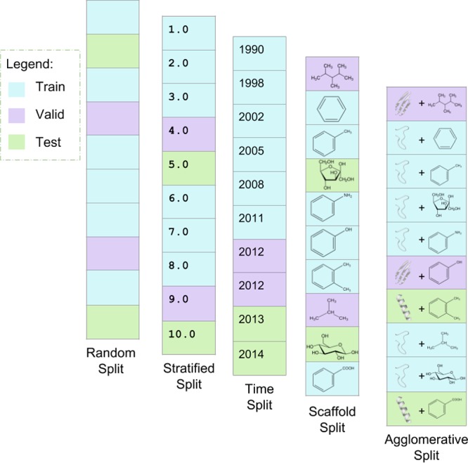
Notional comparison of cross-validation splitting algorithms. The first four vertical panels from the left depict simple examples of random split, stratified split, time split, and scaffold split. The rightmost panel depicts a toy example of the agglomerative split proposed in this work. Both scaffold split and agglomerative split group similar data points together to promote the generalizability of the network to new data. Scaffold split uses the algorithm introduced by Bemis and Murcko47 to group ligands into common frameworks. The agglomerative split uses hierarchical agglomerative clustering to group ligand–protein systems according to pairwise sequence or structural similarity of the proteins. This figure is adapted from ref (3) with permission from the Royal Society of Chemistry.
IV.B. Performance of Methods on Benchmarks
On the standard PDBBind 2007 “Refined Train, Core Test” benchmark, the PotentialNet Spatial Graph Convolution achieves state-of-the-art performance as reflected by several metrics. PotentialNet outperforms RF-Score and X-Score according to Pearson and Spearman correlation coefficients. The Pearson correlation score for eqs 7–9 is within error of the reported score for TopologyNet, the heretofore top performing model on this benchmark. However, a key caveat must be noted with respect to this comparison: all cross-validation for this Article, including all of our results reported in Tables 1–3, was performed such that performance on the test set was recorded for the hyperparameter set that performed most highly on the validation set. In contrast, in the TopologyNet study,37 models were trained on a combination of the validation and training sets and evaluated directly on the test set. Performance for TopologyNet37 therefore reflects a train–validation type split rather than a train–validation–test split, which likely inflated the performance of that method.
Table 1. Benchmark: PDBBind 2007, Refined Train, Core Testa.
| model | Test R2 | Test EFχ(R) | Test Pearson | Test Spearman | Test stdev | Test MUE |
|---|---|---|---|---|---|---|
| PotentialNet | 0.668 (0.043) | 1.643 (0.127) | 0.822 (0.021) | 0.826 (0.020) | 1.388 (0.070) | 0.626 (0.037) |
| PotentialNet, (ligand-only control) | 0.419 (0.234) | 1.404 (0.171) | 0.650 (0.017) | 0.670 (0.014) | 1.832 (0.135) | 0.839 (0.005) |
| TopologyNet, no validation set | N/A | N/A | 0.826 | N/A | N/A | N/A |
| RF-Score | N/A | N/A | 0.783 | 0.769 | N/A | N/A |
| X-Score | N/A | N/A | 0.643 | 0.707 | N/A | N/A |
Error bars are recorded as standard deviation of the test metric over three random initializations of the best model as determined by average validation set score. MUE is mean unsigned error. Pearson test scores for TopologyNet are reported from ref (37), and RF- and X-Scores are reported from ref (44).
Table 3. Benchmark: PDBBind 2007 Refined, Agglomerative Structure Splita.
| model | Test R2 | Test EFχ(R) | Test Pearson | Test Spearman | Test MUE |
|---|---|---|---|---|---|
| PotentialNet | 0.629 (0.044) | 1.576 (0.053) | 0.823 (0.023) | 0.805 (0.019) | 1.553 (0.125) |
| ligand-only PotentialNet | 0.500 (0.010) | 1.498 (0.411) | 0.733 (0.007) | 0.726 (0.005) | 1.700 (0.067) |
| RF-Score | 0.594 (0.005) | 0.869 (0.090) | 0.779 (0.003) | 0.757 (0.005) | 1.542 (0.046) |
| X-Score | 0.517 | 0.891 | 0.730 | 0.751 | 1.751 |
Error bars are recorded as standard deviation of the test metric over three random initializations of the best model as determined by average validation set score. MUE is mean unsigned error. X-Score does not have error because it is a deterministic linear model.
Intriguingly, the gap in performance between the PotentialNet Spatial Graph Convolution and the other tested statistical models changes considerably on the agglomerative structure and sequence split benchmarks. On sequence split, RF-Score achieves the best overall performance, followed by a statistical tie between the Staged Spatial Graph Convolution, eqs 7–9 , and X-Score, followed by the ligand-only graph convolutional control. Meanwhile, on structure split, PotentialNet achieves the highest overall performance, followed by RF-Score, followed by a statistical tie of X-Score, and the graph convolutional ligand-only control.
It is noteworthy that the PotentialNet Spatial Graph Convolutions (eqs 7–9) perform competitively with other compared methods when the proposed Spatial Graph Convolutions are predicated on very simple, per-atom features and pure notions of distance whereas RF-Score, X-Score, and TopologyNet all directly incorporate domain-expertise-driven information on protein–ligand interactions.
IV.B.1. Sanity Check with a Traditional RNN
Given the unreasonable effectiveness of deep learning methods in mostly unstructured settings, it is important to justify our incorporation of domain knowledge over a purely deep learning-based approach. To do this, we trained a bidirectional long short-term memory (LSTM) network, a commonly used recurrent neural network (RNN) that handles both past and future context well. We represented the protein–ligand complexes using a sequential representation of protein–ligand complexes in PDBBind: proteins were one-hot encoded by amino acid, and ligands were similarly encoded on a character-level using their SMILES string representation. The test Pearson correlation coefficient corresponding to the best validation score (using the same metric) was 0.518, far worse than our results and justifying our model’s incorporation of domain knowledge.
IV.C. Ligand-Based Models
While crystallography, NMR, and, most recently, cryoelectron microscopy have opened a new paradigm of structure-based drug design, many critical tasks of drug discovery can be predicted from the chemical composition of a given molecule itself, without explicit knowledge of the macromolecule(s) to which they bind. Such properties include electronic spectra (important for parametrizing small molecule force fields for molecular dynamics simulations, for example), solubility, and animal toxicity.
Quantum mechanical data sets are particularly ripe for machine learning algorithms since it is straightforward to generate training data at some known accuracy. The QM8 data set,48 which contains several electronic properties for small molecules in the GDB-8 set, lends itself particularly well for benchmarking PotentialNet eqs 7–9 since each compound’s properties are calculated based on the three-dimensional coordinates of each element. The ESOL solubility49 and Tox21 toxicity50 data sets map two-dimensional molecular representations consisting solely of atoms and their bonds to their respective single-task and multitask outputs, and therefore serve as validation of our neural network implementations as well as of the value of incorporating nonlinearity into the message function.
To summarize, our computational experiments indicate that PotentialNet leads to statistically significant improvements in performance for all three investigated ligand-based tasks. For the QM8 data set, we were able to directly assess the performance benefit that stems from separating spatial graph convolutions into distinct stages. Recall that stage I of PotentialNet, eq 7, propagates information over only bonds and therefore derives differentiable “atom types”, whereas stage II of PotentialNet, eq 8, propagates information over both bonds and different binned distances. We performed an experiment with QM8 in which stage I was essentially skipped, and graph convolutions propagated both covalent and noncovalent interactions without a privileged first stage for only covalent interactions. Clearly, separating the two stages led to a significant boost in performance.
For each ligand model investigation we benchmark against the error suggested upon introduction of the data set, or to enable direct comparison with previously published approaches. For extensive benchmarking of various models on these and other data sets, we refer the reader to ref (3).
IV.C.1. Quantum Property Prediction
Table 4 reports the performances in mean absolute error (MAE) over 21 786 compounds and 12 tasks in QM8. We utilize MAE for consistency with the original proposal of the database.48 Multiple PotentialNet variants and two mature deep learning models, deep tensor neural network51 (DTNN) and message passing neural network8 (MPNN), are evaluated, in which the latter two models proved to be successful on quantum mechanical tasks (e.g., atomization energy3). We restricted the training length to 100 epochs and performed 100 rounds of hyperparameter search on PotentialNet models. The staged spatial PotentialNet model achieved the best performances in the group, demonstrating strong predictive power on the tasks. We have also included taskwise results in Appendix B.
Table 4. Quantum Property Prediction with QM8 Data Seta.
| network | Valid MAE | Test MAE |
|---|---|---|
| spatial PotentialNet, staged | 0.0120 | 0.0118 (0.0003) |
| spatial PotentialNet, SingleUpdate | 0.0133 | 0.0131 (0.0001) |
| MPNN | 0.0142 | 0.0139 (0.0007) |
| DTNN | 0.0168 | 0.0163 (0.0010) |
Error bars are recorded as standard deviation of the test metric over three random initializations of the best model as determined by average validation set score.
IV.C.2. Toxicity
In the multitask toxicity benchmark, we evaluated the performances of two graph convolutional type models5,16 and PotentialNet on the Tox21 data set under the same evaluation pattern (see Table 5). With 100 epochs of training, PotentialNet demonstrated higher ROC–AUC scores on both validation and test scores, outperforming Weave and GraphConv by a comfortable margin.
Table 5. Toxicity Prediction with the Tox21 Data Seta.
| network | Valid ROC–AUC | Test ROC–AUC |
|---|---|---|
| PotentialNet | 0.878 | 0.857 (0.006) |
| Weave | 0.852 | 0.831 (0.013) |
| GraphConv | 0.858 | 0.838 (0.001) |
| XGBoost | 0.778 | 0.808 (0.000) |
Error bars are recorded as standard deviation of the test metric over three random initializations of the best model as determined by average validation set score.
IV.C.3. Solubility
The same three models are also tested and compared on a solubility task,49 using RMSE to quantify the error to compare to previous work.16 PotentialNet achieved slightly smaller RMSE than Weave and GraphConv (Table 6). Under the limited 100 epochs training, the final test RMSE is comparable or even superior to the best scores reported for Weave and GraphConv (0.465 and 0.52,16 respectively).
Table 6. Solubility Prediction with the Delaney ESOL Data Seta.
| network | Valid RMSE | Test RMSE |
|---|---|---|
| PotentialNet | 0.517 | 0.490 (0.014) |
| Weave | 0.549 | 0.553 (0.035) |
| GraphConv | 0.721 | 0.648 (0.019) |
| XGBoost | 1.182 | 0.912 (0.000) |
Error bars are recorded as standard deviation of the test metric over three random initializations of the best model as determined by average validation set score.
V. Discussion
Spatial Graph Convolutions exhibit state-of-the-art performance in affinity prediction. Whether based on linear regression, random forests, or other classes of DNNs, all three of RF-Score, X-Score, and TopologyNet are machine learning models that explicitly draw upon traditional physics-based features. Meanwhile, the Spatial Graph Convolutions presented here use a more principled deep learning approach. Input features are only basic information about atoms, bonds, and distances. This framework does not use traditional hand-crafted features, such as hydrophobic effects, π-stacking, or hydrogen bonding. Instead, higher-level interaction “features” are learned through intermediate graph convolutional neural network layers.
The traditional PDBBind 2007 benchmark uses 1105 samples from the refined set for training and 195 from the core set for testing. Here, Spatial Graph Convolutions outperform X-Score and RF-Score and perform comparably with TopologyNet (even though this searched hyperparameters directly over the test data set). On our proposed agglomerative clustering cross-validation benchmark, the choice of sequence or structure split affects relative performance. On sequence split, RF-Score achieved the highest overall performance, with Staged Spatial Graph Convolutions and X-Score statistically tied for second. However, on structure split, the Staged Spatial Graph Convolutions performed best, with RF-Score in second place.
While the Pearson correlation was employed in the preceding performance comparison, instead, comparing methods through EFχ(R) tells a mildly different story. On the agglomerative sequence cross-validation split, in which test proteins are separated from train proteins based on amino acid sequence deviation, X-Score statistically ties RF-Score for the best model, while PotentialNet statistically ties the ligand-only PotentialNet control for last place at over 0.1 average standard deviations worse than X-Score and RF-Score for the top 5% of predictions. Meanwhile, using the agglomerative structure cross-validation split, PotentialNet exceeds the performance of X-Score and RF-Score by over 0.5 average standard deviations, although it is within a statistical tie of the ligand-only PotentialNet control (which has a surprisingly high variance in its EFχ). Taken together, we aver that it is important for the future of ML-driven structure-based drug discovery to carefully choose both (1) the cross-validation technique and (2) the metric of performance on held-out test set to most accurately reflect the capacity of their models to generalize in simulated realistic settings.
In light of the continued importance and success of ligand-based methods in drug discovery, we benchmarked PotentialNet on several ligand based tasks: electronic property (multitask), solubility (single task), and toxicity prediction (multitask). Statistically significant performance increases were observed for all three prediction tasks. A potentially step change improvement was observed for the QM8 challenge which also reinforced the value of the concept of stages that privilege bonded from nonbonded interactions (see Table 4).
Despite the simpler input featurization, Spatial Graph Convolutions can learn an accurate mapping of protein–ligand structures to binding free energies using the same relatively low amount of data as previous expertise-driven approaches. We thus expect that as larger sets of training data become available, Spatial Graph Convolutions can become the gold standard in affinity prediction. Unfortunately, such larger, publicly available data sets are currently nonexistent. We thus call upon academic experimental scientists and/or their pharmaceutical industry counterparts to release as much high-quality protein–ligand binding affinity data as possible so the community can develop and benefit from better affinity prediction models.
Due to the field’s immense practical applications, our algorithms must prioritize realizable results over incremental improvements on somewhat arbitrary benchmarks. We thus also present a new benchmark score and accompanying cross-validation procedure. The latter draws on agglomerative clustering of sequence and structural similarity to construct challenging train–test splits. Using this proposed cross-validation schema, on sequence-based splitting (Table 2) we observe in the Pearson correlation column that RF-Score exceeds X-Score, and X-Score statistically ties Spatial Graph Convolutions. For structure-based splitting (Table 3) we observe that Spatial Graph Convolutions exceeds both RF-Score and X-Score in the Pearson correlation column. We highlight the Pearson correlation for consistency with the literature, but present other metrics in Tables 2 and 3 from which similar conclusions could be drawn.
Table 2. Benchmark: PDBBind 2007 Refined, Agglomerative Sequence Splita.
| model | Test R2 | Test EFχ(R) | Test Pearson | Test Spearman | Test MUE |
|---|---|---|---|---|---|
| PotentialNet | 0.480 (0.030) | 0.867 (0.036) | 0.700 (0.003) | 0.694 (0.012) | 1.680 (0.061) |
| ligand-only PotentialNet | 0.414 (0.058) | 0.883 (0.025) | 0.653 (0.031) | 0.674 (0.020) | 1.712 (0.110) |
| RF-Score | 0.527 (0.014) | 1.078 (0.143) | 0.732 (0.009) | 0.723 (0.013) | 1.582 (0.034) |
| X-Score | 0.470 | 1.117 | 0.702 | 0.764 | 1.667 |
Error bars are recorded as standard deviation of the test metric over three random initializations of the best model as determined by average validation set score. MUE is mean unsigned error. X-Score does not have error because it is a deterministic linear model.
This construction (i.e., choice of cross-validation schema) helps assess models with a practical test set, such as one containing newly designed compounds on previously unseen protein targets. Although standard machine learning practice draws train and test sets from the same distribution, if machine leaning is to be applied to real-world drug discovery settings it is imperative that we accurately measure a given model’s capacity both to interpolate within familiar regions of chemical space as well as to generalize to its less charted territories.
VI. Methods
VI.A. Models
DNNs were constructed and trained with PyTorch.52 Custom Python code was used based on RDKit53 and OEChem54 with frequent use of NumPy55 and SciPy.56 Networks were trained on chemical element, formal charge, hybridization, aromaticity, and the total numbers of bonds, hydrogens (total and implicit), and radical electrons. Random forest and linear regression models (i.e., X-Score) were implemented using scikit-learn;57 all random forests models were trained with 500 trees and 6 features per tree, and the implementation of X-Score is described in ref (44). Hyperparameters for PotentialNet models trained for binding affinity, electronic properties, toxicity, and solubility studies are given in Table 7; for toxicity and solubility models, only bond graph convolution layers are employed since there are no 3D coordinates provided for the associated data sets. For these three tasks, random splitting was used for cross-validation. For the RNN sanity check of the ligand binding task, the best-performing LSTM sanity check was constructed with 5 layers, a hidden size of 32, 10 classes, and a learning rate of 3.45e–4.
Table 7. Hyperparameters for Neural Networks (equations 7–9).
| network | hyperparameter name | symbol | possible values |
|---|---|---|---|
| PotentialNet | gather widths (bond and spatial) | fbond, fspatial | [64, 128] |
| PotentialNet | number of bond convolution layers | bondK | [1, 2] |
| PotentialNet | number of spatial convolution layers | spatialK | [1, 2, 3] |
| PotentialNet | gather width | fgather | [64, 128] |
| PotentialNet | number of graph convolution layers | K | [1, 2, 3] |
| both | fully connected widths | nrows of W(FCi) | [[128, 32, 1], [128, 1], [64, 32, 1], [64, 1]] |
| both | learning rate | [1e–3, 2e–4] | |
| both | weight decay | [0., 1e–7, 1e–5, 1e–3] | |
| both | dropout | [0., 0.25, 0.4, 0.5] |
VI.B. Cross-Validation on PDBBind 2007 Core Test Set Benchmark
The core set was removed from the refined set sorted temporally to create the test set. Up to 8 hyperparameters were tuned through random search. K-fold temporal cross-validation was conducted within the train set for each hyperparameter set. For each held-out fold, validation set performance was recorded at the epoch with maximal Pearson correlation coefficient between the labeled and predicted values in the validation set. For each hyperparameter set, the validation score was the average Pearson score over the K folds using the best epoch for each fold. The set with the best validation score was then used to evaluate test performance. The training set was split into K temporal folds; for each fold, test set performance was recorded at the epoch with highest validation score. All reported metrics are given as the median with the standard deviation over K folds in parentheses.
VI.C. Cross-Validation on PDBBind 2007 Structure and Sequence Agglomerative Clustering Split Benchmarks
Agglomerative clustering was performed with Ward’s method.58 Pairwise distance between PDB proteins was measured as either 1.0 minus the sequence homology or the TMScore.59 Within the train set, for each hyperparameter set, K random splits within the train set were performed. For each held-out fold, validation set performance was recorded at the epoch with maximal Pearson correlation coefficient. The set with the best average Pearson score on the validation set was used to evaluate test set performance. The training set was again randomly split into K folds; for each fold, test set performance was recorded at the epoch at which the held-out performance was highest according to Pearson score. Metrics are reported as detailed above.
Acknowledgments
We are grateful to the anonymous reviewers for their suggestions. E.N.F. is supported by the Blue Waters Graduate Fellowship. Y.L., S.S., and J.Y. acknowledge the support of the National Natural Science Foundation of China (11501306) and the Fok Ying-Tong Education Foundation (161003). B.R. was supported by the Fannie and John Hertz Foundation. The Pande Group acknowledges the generous support of Dr. Anders G. Frøseth and Mr. Christian Sundt for our work on machine learning. The Pande Group is broadly supported by grants from the NIH (R01 GM062868 and U19 AI109662) as well as gift funds and contributions from Folding@home donors.
Appendix A: Computational Complexity of Network Architectures
Here, we consider the complexity of the various
neural architectures
discussed in Section II, starting with the simple fully connected setting. Forward propagation
can be understood as passing an input vector x of
length n through h matrix multiplications,
each  , and h elementwise nonlinear
activation layers, each
  . Assuming h ≪ n, this yields a total complexity of
  . Since back-propagation involves the same
dimensions and number of layers, just in reverse order, it has the
same complexity as the forward operation.
Complexity analysis
for a 2D convolutional neural network, typical
in computer vision tasks, is a bit more involved. An m- × n-dimensional filter on an M × N image yields m × n computations on M × N pixels, in total  . Using the fast Fourier transform for optimized
processing, a single convolutional layer will be
  , the same complexity as the entire
network.
Notice that these operations’ costs grow exponentially with
the dimension of Euclidean data—making the exploitation of
symmetry far more important for 3D graph data.
The GGNN family
of graph convolutional architectures includes effective
optimizations to reduce complexity on graphs. Let d be the dimension of each node’s internal hidden representation
and n be the number of nodes in the graph. A single
step of message passing for a dense graph requires  multiplications. Breaking the d dimensional node embeddings into k different
  dimensional embeddings reduces
this runtime
to
  . As most molecules are sparse or relatively
small graphs, these layers are typically
  . Although other optimizations exist, such
as utilizing spectral representations of graphs, the models presented
in this work build around this general GGNN framework with different
nonlinearities and update rules. None of these are sufficiently computationally
expensive enough to alter the total runtime.
Appendix B: Taskwise Results for Quantum Property Prediction
In Table 8 we have recorded the test set performances for all 12 tasks in the QM8 data set using the MAE for a deep tensor neural network51 (DTNN), a message passing neural network8 (MPNN), and the staged and single update Spatial PotentialNet networks as in Section II.B.1.
Table 8. QM8 Test Set Performances of All Tasks (Mean Absolute Error).
| task | DTNN | MPNN | PotentialNet, single update | PotentialNet, staged |
|---|---|---|---|---|
| E1–CC2 | 0.0092 | 0.0084 | 0.0070 | 0.0068 |
| E2–CC2 | 0.0092 | 0.0091 | 0.0079 | 0.0074 |
| f1–CC2 | 0.0182 | 0.0151 | 0.0137 | 0.0134 |
| f2–CC2 | 0.0377 | 0.0314 | 0.0296 | 0.0285 |
| E1–PBE0 | 0.0090 | 0.0083 | 0.0070 | 0.0067 |
| E2–PBE0 | 0.0086 | 0.0086 | 0.0074 | 0.0070 |
| f1–PBE0 | 0.0155 | 0.0123 | 0.0112 | 0.0108 |
| f2–PBE0 | 0.0281 | 0.0236 | 0.0228 | 0.0215 |
| E1–CAM | 0.0086 | 0.0079 | 0.0066 | 0.0063 |
| E2–CAM | 0.0082 | 0.0082 | 0.0069 | 0.0064 |
| f1–CAM | 0.0180 | 0.0134 | 0.0123 | 0.0117 |
| f2–CAM | 0.0322 | 0.0258 | 0.0245 | 0.0233 |
Supporting Information Available
The Supporting Information is available free of charge on the ACS Publications website at DOI: 10.1021/acscentsci.8b00507.
Sequence- and structure-based agglomerative clustering cross-validation splittings for the PDBBind 2007 refined set (TXT)
The authors declare the following competing financial interest(s): V.S.P. is a consultant & SAB member of Schrodinger, LLC and Globavir, sits on the Board of Directors of Apeel Inc, Asimov Inc, BioAge Labs, Freenome Inc, Omada Health, Patient Ping, and Rigetti Computing, and is a General Partner at Andreessen Horowitz.
Notes
Safety statement: no unexpected or unusually high safety hazards were encountered in this study.
Supplementary Material
References
- Deng J.; Dong W.; Socher R.; Li L.; Li K.; Fei-Fei L. ImageNet: A large-scale hierarchical image database. 2009 IEEE Conference on Computer Vision and Pattern Recognition 2009, 248. 10.1109/CVPR.2009.5206848. [DOI] [Google Scholar]
- Liu Z.; Su M.; Han L.; Liu J.; Yang Q.; Li Y.; Wang R. Forging the basis for developing protein–ligand interaction scoring functions. Acc. Chem. Res. 2017, 50, 302–309. 10.1021/acs.accounts.6b00491. [DOI] [PubMed] [Google Scholar]
- Wu Z.; Ramsundar B.; Feinberg E. N.; Gomes J.; Geniesse C.; Pappu A. S.; Leswing K.; Pande V. MoleculeNet: A benchmark for molecular machine learning. Chem. Sci. 2018, 9, 513–530. 10.1039/C7SC02664A. [DOI] [PMC free article] [PubMed] [Google Scholar]
- Hastie T.; Tibshirani R.; Friedman J.. The Elements of Statistical Learning; Springer Series in Statistics: New York, NY, 2009; pp 9–41. [Google Scholar]
- Kearnes S.; McCloskey K.; Berndl M.; Pande V.; Riley P. Molecular graph convolutions: Moving beyond fingerprints. J. Comput.-Aided Mol. Des. 2016, 30, 595–608. 10.1007/s10822-016-9938-8. [DOI] [PMC free article] [PubMed] [Google Scholar]
- Kipf T. N.; Welling M.. Semi-supervised classification with graph convolutional networks. 2016, arXiv:1609.02907. arXiv.org e-Print archive. https://arxiv.org/abs/1609.02907.
- Li Y.; Zemel R.; Brockschmidt M.; Tarlow D. Proceedings of the International Conference on Learning Representations 2016, San Juan, Puerto Rico, May 2–4, 2016.
- Gilmer J.; Schoenholz S. S.; Riley P. F.; Vinyals O.; Dahl G. E.. Neural message passing for quantum chemistry. Proceedings of the 34th International Conference on Machine Learning, International Convention Centre, Sydney, Australia, 2017; pp 1263–1272.
- Morgan H. The generation of a unique machine description for chemical structures-a technique developed at chemical abstracts service. J. Chem. Doc. 1965, 5, 107–113. 10.1021/c160017a018. [DOI] [Google Scholar]
- Weininger D.; Weininger A.; Weininger J. L. SMILES. 2. Algorithm for generation of unique SMILES notation. J. Chem. Inf. Model. 1989, 29, 97–101. 10.1021/ci00062a008. [DOI] [Google Scholar]
- Ullmann J. R. An algorithm for subgraph isomorphism. J. Assoc. Comput. Mach. 1976, 23, 31–42. 10.1145/321921.321925. [DOI] [Google Scholar]
- Rogers D.; Hahn M. Extended-connectivity fingerprints. J. Chem. Inf. Model. 2010, 50, 742–754. 10.1021/ci100050t. [DOI] [PubMed] [Google Scholar]
- Hawkins P. C.; Skillman A. G.; Nicholls A. Comparison of shape-matching and docking as virtual screening tools. J. Med. Chem. 2007, 50, 74–82. 10.1021/jm0603365. [DOI] [PubMed] [Google Scholar]
- Kearnes S.; Pande V. ROCS-derived features for virtual screening. J. Comput.-Aided Mol. Des. 2016, 30, 609–617. 10.1007/s10822-016-9959-3. [DOI] [PubMed] [Google Scholar]
- Krizhevsky A.; Sutskever I.; Hinton G. E. In Advances in Neural Information Processing Systems 25; Pereira F., Burges C. J. C., Bottou L., Weinberger K. Q., Eds.; Curran Associates, Inc.: Lake Tahoe, NV, 2012; pp 1097–1105. [Google Scholar]
- Duvenaud D. K.; Maclaurin D.; Iparraguirre J.; Bombarell R.; Hirzel T.; Aspuru-Guzik A.; Adams R. P. In Advances in Neural Information Processing Systems 28; Cortes C., Lawrence N. D., Lee D. D., Sugiyama M., Garnett R., Eds.; Curran Associates, Inc.; Montréal, Canada, 2015; pp 2224–2232. [Google Scholar]
- Perutz M. F.; Rossmann M. G.; Cullis A. F.; Muirhead H.; Will G.; North A. Structure of hæmoglobin: A three-dimensional Fourier synthesis at 5.5-Å. resolution, obtained by X-ray analysis. Nature 1960, 185, 416–422. 10.1038/185416a0. [DOI] [PubMed] [Google Scholar]
- Jain A. N. Surflex: Fully automatic flexible molecular docking using a molecular similarity-based search engine. J. Med. Chem. 2003, 46, 499–511. 10.1021/jm020406h. [DOI] [PubMed] [Google Scholar]
- Shoichet B. K.; Kuntz I. D.; Bodian D. L. Molecular docking using shape descriptors. J. Comput. Chem. 1992, 13, 380–397. 10.1002/jcc.540130311. [DOI] [Google Scholar]
- Trott O.; Olson A. J. AutoDock Vina: Improving the speed and accuracy of docking with a new scoring function, efficient optimization, and multithreading. J. Comput. Chem. 2010, 31, 455–461. 10.1002/jcc.21334. [DOI] [PMC free article] [PubMed] [Google Scholar]
- Friesner R. A.; et al. Glide: A new approach for rapid, accurate docking and scoring. 1. Method and assessment of docking accuracy. J. Med. Chem. 2004, 47, 1739–1749. 10.1021/jm0306430. [DOI] [PubMed] [Google Scholar]
- Wang L.; et al. Accurate and reliable prediction of relative ligand binding potency in prospective drug discovery by way of a modern free-energy calculation protocol and force field. J. Am. Chem. Soc. 2015, 137, 2695–2703. 10.1021/ja512751q. [DOI] [PubMed] [Google Scholar]
- Hensen C.; Hermann J. C.; Nam K.; Ma S.; Gao J.; Höltje H.-D. A combined QM/MM approach to protein-ligand interactions: Polarization effects of the HIV-1 protease on selected high affinity inhibitors. J. Med. Chem. 2004, 47, 6673–6680. 10.1021/jm0497343. [DOI] [PubMed] [Google Scholar]
- Li H.; Leung K.-S.; Wong M.-H.; Ballester P. J. Improving AutoDock Vina using random forest: the growing accuracy of binding affinity prediction by the effective exploitation of larger data sets. Mol. Inf. 2015, 34, 115–126. 10.1002/minf.201400132. [DOI] [PubMed] [Google Scholar]
- Ballester P. J.; Mitchell J. B. A machine learning approach to predicting protein–ligand binding affinity with applications to molecular docking. Bioinformatics 2010, 26, 1169–1175. 10.1093/bioinformatics/btq112. [DOI] [PMC free article] [PubMed] [Google Scholar]
- Durrant J. D.; McCammon J. A. NNScore 2.0: A neural-network receptor–ligand scoring function. J. Chem. Inf. Model. 2011, 51, 2897–2903. 10.1021/ci2003889. [DOI] [PMC free article] [PubMed] [Google Scholar]
- Wallach I.; Dzamba M.; Heifets A.. AtomNet: A deep convolutional neural network for bioactivity prediction in structure-based drug discovery. 2015, arXiv:1510.02855. arXiv.org e-Print archive. https://arxiv.org/abs/1510.02855.
- Ragoza M.; Hochuli J.; Idrobo E.; Sunseri J.; Koes D. R. Protein–ligand scoring with convolutional neural networks. J. Chem. Inf. Model. 2017, 57, 942–957. 10.1021/acs.jcim.6b00740. [DOI] [PMC free article] [PubMed] [Google Scholar]
- Gomes J.; Ramsundar B.; Feinberg E. N.; Pande V. S.. Atomic convolutional networks for predicting protein-ligand binding affinity. 2017, arXiv:1703.10603. arXiv.org e-Print archive. https://arxiv.org/abs/1703.10603.
- Ponder J. W.; Case D. A. Force fields for protein simulations. Adv. Protein Chem. 2003, 66, 27–85. 10.1016/S0065-3233(03)66002-X. [DOI] [PubMed] [Google Scholar]
- Triballeau N.; Acher F.; Brabet I.; Pin J.-P.; Bertrand H.-O. Virtual screening workflow development guided by the ’’receiver operating characteristic’’ curve approach. Application to high-throughput docking on metabotropic glutamate receptor subtype 4. J. Med. Chem. 2005, 48, 2534–2547. 10.1021/jm049092j. [DOI] [PubMed] [Google Scholar]
- Truchon J.-F.; Bayly C. I. Evaluating virtual screening methods: good and bad metrics for the ’’early recognition’’ problem. J. Chem. Inf. Model. 2007, 47, 488–508. 10.1021/ci600426e. [DOI] [PubMed] [Google Scholar]
- Mysinger M. M.; Shoichet B. K. Rapid context-dependent ligand desolvation in molecular docking. J. Chem. Inf. Model. 2010, 50, 1561–1573. 10.1021/ci100214a. [DOI] [PubMed] [Google Scholar]
- EFχ(R) values may therefore exceed 1.0, since this means that the χ percentage of top predicted molecules have an average standard deviation of more than 1.0 above the mean.
- Boulesteix A.-L. Ten simple rules for reducing overoptimistic reporting in methodological computational research. PLoS Comput. Biol. 2015, 11, e1004191. 10.1371/journal.pcbi.1004191. [DOI] [PMC free article] [PubMed] [Google Scholar]
- Chicco D. Ten quick tips for machine learning in computational biology. BioData Min. 2017, 10, 35. 10.1186/s13040-017-0155-3. [DOI] [PMC free article] [PubMed] [Google Scholar]
- Cang Z.; Wei G. TopologyNet: Topology based deep convolutional and multi-task neural networks for biomolecular property predictions. PLoS Comput. Biol. 2017, 13, e1005690. 10.1371/journal.pcbi.1005690. [DOI] [PMC free article] [PubMed] [Google Scholar]
- Jiménez J.; Skalic M.; Martínez-Rosell G.; De Fabritiis G. K. DEEP: Protein-ligand absolute binding affinity prediction via 3D-convolutional neural networks. J. Chem. Inf. Model. 2018, 58, 287–296. 10.1021/acs.jcim.7b00650. [DOI] [PubMed] [Google Scholar]
- Wang R.; Fang X.; Lu Y.; Wang S. The PDBbind database: Collection of binding affinities for protein–ligand complexes with known three-dimensional structures. J. Med. Chem. 2004, 47, 2977–2980. 10.1021/jm030580l. [DOI] [PubMed] [Google Scholar]
- Wang R.; Fang X.; Lu Y.; Yang C.-Y.; Wang S. The PDBbind database: Methodologies and updates. J. Med. Chem. 2005, 48, 4111–4119. 10.1021/jm048957q. [DOI] [PubMed] [Google Scholar]
- Wang R.; Lai L.; Wang S. Further development and validation of empirical scoring functions for structure-based binding affinity prediction. J. Comput.-Aided Mol. Des. 2002, 16, 11–26. 10.1023/A:1016357811882. [DOI] [PubMed] [Google Scholar]
- Wang R.; Lu Y.; Wang S. Comparative evaluation of 11 scoring functions for molecular docking. J. Med. Chem. 2003, 46, 2287–2303. 10.1021/jm0203783. [DOI] [PubMed] [Google Scholar]
- Martin E. J.; Polyakov V. R.; Tian L.; Perez R. C. Profile-QSAR 2.0: Kinase virtual screening accuracy comparable to four-concentration IC50s for realistically novel compounds. J. Chem. Inf. Model. 2017, 57, 2077–2088. 10.1021/acs.jcim.7b00166. [DOI] [PubMed] [Google Scholar]
- Li Y.; Yang J. Structural and sequence similarity makes a significant impact on machine-learning-based scoring functions for protein–ligand interactions. J. Chem. Inf. Model. 2017, 57, 1007–1012. 10.1021/acs.jcim.7b00049. [DOI] [PubMed] [Google Scholar]
- Husic B. E.; Pande V. S.. Unsupervised learning of dynamical and molecular similarity using variance minimization. 2017, arXiv:1712.07704. arXiv.org e-Print archive. https://arxiv.org/abs/1712.07704.
- Kramer C.; Gedeck P. Leave-cluster-out cross-validation is appropriate for scoring functions derived from diverse protein data sets. J. Chem. Inf. Model. 2010, 50, 1961–1969. 10.1021/ci100264e. [DOI] [PubMed] [Google Scholar]
- Bemis G. W.; Murcko M. A. The properties of known drugs. 1. Molecular frameworks. J. Med. Chem. 1996, 39, 2887–2893. 10.1021/jm9602928. [DOI] [PubMed] [Google Scholar]
- Ramakrishnan R.; Hartmann M.; Tapavicza E.; von Lilienfeld O. A. Electronic spectra from TDDFT and machine learning in chemical space. J. Chem. Phys. 2015, 143, 084111. 10.1063/1.4928757. [DOI] [PubMed] [Google Scholar]
- Delaney J. S. ESOL: Estimating aqueous solubility directly from molecular structure. J. Chem. Inf. Comput. Sci. 2004, 44, 1000–1005. 10.1021/ci034243x. [DOI] [PubMed] [Google Scholar]
- Tice R. R.; Austin C. P.; Kavlock R. J.; Bucher J. R. Improving the human hazard characterization of chemicals: A Tox21 update. Environ. Health Perspect. 2013, 121, 756. 10.1289/ehp.1205784. [DOI] [PMC free article] [PubMed] [Google Scholar]
- Schütt K. T.; Arbabzadah F.; Chmiela S.; Müller K. R.; Tkatchenko A. Quantum-chemical insights from deep tensor neural networks. Nat. Commun. 2017, 8, 13890. 10.1038/ncomms13890. [DOI] [PMC free article] [PubMed] [Google Scholar]
- Paszke A.; Gross S.; Chintala S.; Chanan G.; Yang E.; DeVito Z.; Lin Z.; Desmaison A.; Antiga L.; Lerer A. In Neural Information Processing Systems Autodiff Workshop, Long Beach, CA, USA, December 9, 2017; Wiltschko A., van Merriënboer B., Lamblin P., Eds.; 2017; https://openreview.net/pdf?id=BJJsrmfCZ (accessed September 10, 2018).
- RDKit: Open-Source Cheminformatics Software. http://www.rdkit.org (accessed September 10, 2018).
- OEChem OpenEye Scientific Software, Santa Fe, NM. http://www.eyesopen.com (accessed September 10, 2018).
- van der Walt S.; Colbert S. C.; Varoquaux G. The NumPy array: a structure for efficient numerical computation. Comput. Sci. Eng. 2011, 13, 22–30. 10.1109/MCSE.2011.37. [DOI] [Google Scholar]
- Jones E.; Oliphant T.; Peterson P.; et al. SciPy: Open source scientific tools for Python. http://www.scipy.org/ (accessed September 10, 2018).
- Pedregosa F.; Varoquaux G.; Gramfort A.; Michel V.; Thirion B.; Grisel O.; Blondel M.; Prettenhofer P.; Weiss R.; Dubourg V.; Vanderplas J.; Passos A.; Cournapeau D.; Brucher M.; Perrot M.; Duchesnay E. Scikit-learn: Machine learning in Python. J. Mach. Learn. Res. 2011, 12, 2825–2830. [Google Scholar]
- Ward J. H. Hierarchical grouping to optimize an objective function. J. Am. Stat. Assoc. 1963, 58, 236–244. 10.1080/01621459.1963.10500845. [DOI] [Google Scholar]
- Zhang Y.; Skolnick J. Scoring function for automated assessment of protein structure template quality. Proteins: Struct., Funct., Genet. 2004, 57, 702–710. 10.1002/prot.20264. [DOI] [PubMed] [Google Scholar]
Associated Data
This section collects any data citations, data availability statements, or supplementary materials included in this article.


