Parameter estimation of kinetic models from metabolic profiles: two-phase dynamic decoupling method

Abstract

Motivation: Time-series measurements of metabolite concentration have become increasingly more common, providing data for building kinetic models of metabolic networks using ordinary differential equations (ODEs). In practice, however, such time-course data are usually incomplete and noisy, and the estimation of kinetic parameters from these data is challenging. Practical limitations due to data and computational aspects, such as solving stiff ODEs and finding global optimal solution to the estimation problem, give motivations to develop a new estimation procedure that can circumvent some of these constraints.

Results: In this work, an incremental and iterative parameter estimation method is proposed that combines and iterates between two estimation phases. One phase involves a decoupling method, in which a subset of model parameters that are associated with measured metabolites, are estimated using the minimization of slope errors. Another phase follows, in which the ODE model is solved one equation at a time and the remaining model parameters are obtained by minimizing concentration errors. The performance of this two-phase method was tested on a generic branched metabolic pathway and the glycolytic pathway of Lactococcus lactis. The results showed that the method is efficient in getting accurate parameter estimates, even when some information is missing.

Contact: rudi.gunawan@chem.ethz.ch

Supplementary information: Supplementary data are available at Bioinformatics online.

1 INTRODUCTION

Advancements in biological techniques have made time series measurements of metabolite concentration more readily available, providing data for the creation of kinetic metabolic network models in the form of ordinary differential equations (ODEs). Time-course data contain information about the structure and dynamics of the metabolic pathways, but such information is implicit and must be extracted using an inference method. This inverse modeling task has motivated the creation of various methods for parameter estimation and structure identification, as summarized in a recent review (Chou and Voit, 2009). However, the inverse modeling of biological systems is often complicated by the lack of complete data, poor data quality (noise) and the computational difficulty in solving model equations and optimization problems. Existing techniques often fail to yield accurate parameter estimates due to one or a combination of these reasons.

Time-series datasets for metabolites are usually incomplete and noisy due to two roadblocks: complexity and technology. The high complexity of metabolic networks with a large number of metabolites means that the complete measurement of all relevant metabolites is not practically feasible. In addition, in order to accurately capture the dynamic behaviors of metabolites, the time-course data should be measured frequently enough, which often challenges the limit of the available techniques. Furthermore, in experiments, several time points of metabolites could be missing because of various reasons (e.g. human error). While the issue of missing time-points can be partly addressed by data interpolation, the complete loss of data from metabolites poses a more challenging problem in parameter estimation and is the focus of the present work. In few instances, it may be possible to obtain missing metabolite measurements by analyzing the convex basis of the left null space of the stoichiometric matrix, which gives the sets of metabolites whose total weighted concentration is time invariant (Famili and Palsson, 2003).

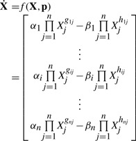
Among canonical ODE models of metabolic networks, power-law models within the Biochemical Systems Theory (BST) (Savageau, 1969a, b), such as S-system, have drawn much attention due to many advantages (Chou and Voit, 2009; Voit, 2000). The generic form of an S-system model is given by:

(1)

where X is an n-dimensional metabolite concentration vector and the parameter vector p consists of the rate constants (α_i, β_i) and kinetic orders (g_ij, h_ij). The sign of the kinetic orders indicates the nature of the connectivity among metabolites, where a positive value represents a substrate or activation and a negative number refers to an inhibition. That is, in S-system models, the parameter values directly describe the connectivity of the metabolic pathway, including stoichiometric and regulatory relationships. This one-to-one relationship between parameters and structural features facilitates parameter estimation and network structure identification in a single step (Sorribas and Cascante, 1994).

One of the challenges when applying standard parameter estimation methods (e.g. least square or maximum likelihood) to S-system models is in the expensive numerical computation of the model solution, where ODE simulations become practically infeasible for some parameter combinations due to stiffness. In one example, the time taken by the ODE integrations in estimating parameters of an S-system model made up >95% of the total computational time (Voit and Almeida, 2004). Another challenge is the combinatorial increase in the number of parameters as a function of the number of metabolites, leading to a large-scale optimization problem. Even after more than 100 publications on this topic, the parameter estimation remains the bottleneck in the application of BST modeling for biochemical networks (Chou and Voit, 2009).

In this article, a new parameter estimation procedure is proposed that combines two methods: the decoupling method (Voit and Almeida, 2004) and the ODE decomposition method (Maki et al., 2002). Provided that all metabolite measurements are available, the decoupling method is a highly efficient estimation procedure that avoids solving ODE integration altogether by fitting models to the slope of time-series data. In the ODE decomposition method, the model equation is solved one at a time, and likewise this method decouples the parameter estimation problem. While each of these methods has its own merits (see Section 2), the proposed iterative estimation is created to keep the advantages and to lessen the disadvantages of the original methods.

2 METHODS

2.1 Decoupling method

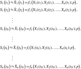
In order to circumvent expensive computational efforts in solving coupled ODEs, a method was proposed previously by fitting the right hand side of the ODE model in Equation (1) to the slope of concentration data directly, thereby decoupling the ODEs (Savageau and Voit, 1982; Voit and Almeida, 2004; Voit and Savageau, 1982a, b):

(2)

Thus, assuming that time-series concentration data of all metabolites X_i(t_k) are available, the slopes S_i(t_k) can be calculated and the estimation simplifies to solving a set of n×N (nonlinear) algebraic equations, where N is the number of time points. Note that since there is no integration of the ODEs, the minimization of the difference between slopes and f(X, p) is computationally efficient, even for a large number of parameters. However, one drawback of this method is that the mole balance is only satisfied at discrete time points t_k and thus, the resulting parameter estimates often give concentration time profiles that offset the data.

When data are noisy, slope estimates by finite differencing will have spurious fluctuations as noise are amplified by such calculations. Thus, data smoothing is a necessary step in this method, for example using polynomial fitting, neural network (Voit and Almeida, 2004) or automated smoother (Vilela et al., 2007). Regardless of the smoothing method, extra care has to be taken to avoid data overfitting, and even with automated methods, user judgment is still needed in this process.

2.2 ODE decomposition method

A different decoupling method has been proposed that involves solving each of the ODE one-by-one, and parameter estimates are obtained by minimizing the sum of squares of concentration difference between model simulations and data (Kimura et al., 2005; Maki et al., 2002; Marino and Voit, 2006). During the integration of one ODE, the other states (metabolites) are treated as external inputs, whose values are interpolated from smoothen time-series data. By solving and fitting one metabolite at a time, this method avoids the integration of coupled ODEs and also reduces the parameter search space. In contrast to the decoupling method above, the mole balance of each metabolite is approximately satisfied over time, not just at discrete time points. Furthermore, the method can still be applied in a situation where there are missing metabolite concentrations. However, the ODE stiffness problem, though lessened, is not completely eliminated.

2.3 Combined iterative estimation

The proposed parameter estimation in this work iterates between the two methods above according to the flowchart shown in Figure 1. By doing so, this method combines the computational efficiency of the decoupling method and reduced search space of the ODE decomposition method, and is also able to handle missing metabolite measurements.

Fig. 1.

Flowchart of the parameter estimation process.

In consideration of missing data of some metabolites, the ODE model is rewritten as:

(3)

where X_m and X_u denote the measured and unmeasured metabolites, respectively, p_m includes all parameters appearing in f_m, and p_u includes the remaining parameters (specific to f_u) and the initial concentrations for X_u. Prior to the iteration, data smoothing was performed to reduce noise effects and to obtain slope estimates. Using the smoothen data and initial guess of the parameters p_u and p_m, a simulation of unmeasured metabolites is carried out by solving the ODEs for X_u only, as done in the ODE decomposition method.

The first iteration then begins with the decoupling method to obtain p_m by minimizing the following slope errors:

(4)

where S_m(t_k) is the slope of smoothen data for X_m at t=t_k. Using the estimates of p_m, the values of p_u are obtained in the next estimation phase by minimizing the concentration errors:

(5)

in which the ODEs are solved one at a time. In this case, the ODEs for X_u are solved prior to X_m and the newly simulated X_u values are then used in the next iteration. If there are more than one unmeasured metabolites, the ODEs for X_u need to be solved simultaneously. The procedure iterates between the two estimation phases until convergence. Here, the iterations are stopped when parameter estimates between iterations differ by less than a chosen convergence factor.

In this article, the optimization problems in the two phases are solved using the SSm GO MATLAB toolbox (Scatter Search Method for Global Optimization) (Egea et al., 2007; Rodriguez-Fernandez et al., 2006). SSm is a population-based metaheuristic method designed to incorporate strategic responses, both deterministic and probabilistic, and has recently been shown to be effective in solving multi-minima optimization problems. In addition, to alleviate the ODE stiffness problem, each ODE simulation is limited to a given maximum time and those exceeding this upper bound are assigned a large objective function value.

3 RESULTS

The performance of the proposed method is demonstrated in applications to a generic branched pathway (Voit and Almeida, 2004) and the glycolytic pathway of Lactococcus lactis (Vilela et al., 2009).

3.1 A generic branched pathway

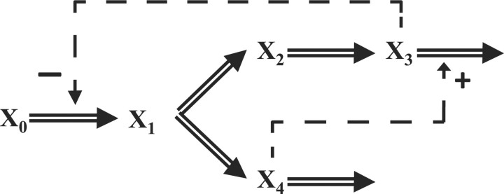
The metabolic pathway in this example is given in Figure 2, which describes the transformations among four metabolites (double-line arrows) with both feedback activation and inhibition (dashed arrows with plus and minus signs, respectively).

Fig. 2.

A generic branched pathway (Voit and Almeida, 2004).

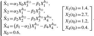
The pathway is modeled in the form of an S-system with 12 kinetic parameters, as follows (Voit and Almeida, 2004):

(6)

This model was used to generate in silico noise-free and noisy experimental data (10% additive noise, Gaussian, i.i.d.) using the parameter values reported in the original publication (see Supplementary Table S1) and with the assumption that only X₁, X₂ and X₄ were measured. A 6th order polynomial, for which the adjusted R² reached a maximum, was chosen for data smoothing and to calculate the slope data. Adjusted R² was used here to avoid data overfitting (Montgomery and Runger, 2007). In the parameter estimation, the search space was limited to α_i, β_i∈[0, 25.0], g_ij, h_ij∈[−2.0, 2.0], and X₃(t₀)∈[0, 5.0]. The numerical integrations were performed in MATLAB using ode15s.

One practical issue affecting the parameter estimation in this example and a majority of biological system modeling is the lack of complete parameter identifiability (Srinath and Gunawan, 2010). In other words, not all parameters can be uniquely identified and only a subset can be determined from data. Here, the proposed method will first be evaluated under the ideal scenario, in which the estimation is done only for the subset of a priori identifiable parameters (AIPs) (Yao et al., 2003) (the other parameters were set to the original values) and using noise-free data. Application of standard least square estimation using fully coupled ODEs encountered numerical stiffness problem and failed to converge, and the decoupling method cannot be applied for estimation involving missing measurements. Thus, in this example, the ODE decomposition estimation was used for comparison.

Table 1 summarizes the estimation results under the ideal scenario described above. In this case, the performance of the proposed method using 0.01% convergence criterion is comparable to the ODE decomposition. The larger parameter deviations in the two-phase estimation is caused by the polynomial smoothing to obtain the time slope data, without which the performance of the two estimation methods are virtually identical. In addition, by increasing the convergence factor, the proposed method can reduce computational time, but at the cost of increased errors in the parameter estimates.

Table 1.

Estimation of AIPs in branched pathway model

	ODE Decomposition	Two-phase estimation
		0.01%a	0.1%a	1%a
Computational time (s)b	3968.33	3741.86 (3823.77)c	2042.40	810.37
Number of stiff simulations	203	0	0	0
Average parameter error (%)	0.24	1.37 (0.20)c	2.26	8.11
Slope errord	2.6435	2.4374 (0.0087)c	2.6052	6.6401
Concentration errore	0.0047	0.0187 (0.0049)c	0.0198	0.0805

^aConvergence criterion between two estimation phases.

^bComputational times were based on Dual Processors Intel Quad-Core 2.83 GHz.

^cEvaluated using actual slope values from the ODEs.

^dSlope error is calculated using Equation (4), in which X_u , X_m are simulated using coupled ODEs.

^eConcentration error is calculated using Equation (5), in which X_m are simulated using coupled ODEs.

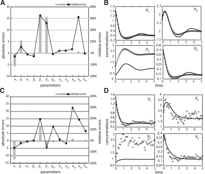
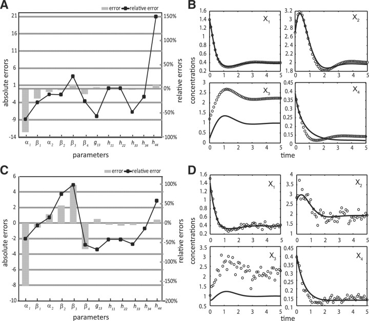
The results of estimating the full parameter set are given in Table 2, Figure 3A–B and Supplementary Table S1. Even when data are noise-free, the relative errors of the parameter estimates can reach higher than 300% using the ODE decomposition method. While parameter identifiability issue certainly contributes to these errors, the ODE decomposition in this case failed to extract the maximum information available in the data, in comparison to the proposed method. Here, the application of the proposed iterative method using noise-free data and 1% convergence criterion gave improved parameter estimates and importantly, in much shorter time than the ODE decomposition (see Figure 4A–B and Table 2). The maximum relative error dropped to 150% and fewer parameters had errors above 50%. In addition, the predicted concentration and slope profiles were relatively better than those from the ODE decomposition alone. While the lack of fit to the missing X₃ data in both methods was expected, parameter estimates from both methods were able to capture the trend.

Table 2.

Parameter estimation of the branched pathway model

	ODE decomposition		Two-phase estimation
	w/o noise	w/ noise	w/o noise	w/ noise
Computational time (s)	4493.2	10910.3	1062.1	2807.4
Number of stiff ODE simulations	1247	2012	359	823
Average parameter error (%)	92.18	90.97	36.59	47.27
Slope error	2.5962	9.4303	0.8620	8.5909
Concentration error	0.5137	5.8207	0.1526	3.6021

Fig. 3.

ODE decomposition estimation in the branched pathway model: parameter errors (A, C) and concentration simulations (B, D) using noise-free (A, B) and noisy data (C, D); (solid line) simulation profile, (open circles) in silico data.

Fig. 4.

Two-phase iterative estimation in the branched pathway model: parameter errors (A, C) and concentration simulations (B, D) using noise-free (A, B) and noisy data (C, D); (solid line) simulation profile, (open circles) in silico data.

The proposed iterative method again gave comparatively more accurate parameter estimates and finished in much shorter time than the ODE decomposition when using noisy data. The results from the two estimation methods are shown in Figures 3C–D and 4C–D and in Table 2. As expected, these parameter estimates were on average less accurate than those obtained from noise-free data. However, the estimation in this case took two to three times longer than those using noise-free data.

3.2 The glycolytic pathway in L.lactis

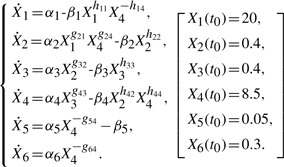
The second case study was taken from the modeling of the glycolytic pathway of L.lactis using S-system (Vilela et al., 2009) (Supplementary Figure S2). Experimental time-course data of the metabolites were previously obtained using in vivo NMR (Neves et al., 2005; Ramos et al., 2002). Here, the concentration variables denote the following metabolites: glucose (Glu)—X₁; glucose 6-phosphate (G6P)—X₂; fructose 1, 6-biphosphate (FBP)—X₃, phosphoenolpyruvate (PEP)—X₄; lactate (Lac)—X₅; and acetate (Ace)—X₆. Assuming that the network connectivity is known, the model equations and initial conditions are given by:

(7)

First, using the parameters reported in the original publication (Vilela et al., 2009) (Supplementary Table S3), in silico noise-free data were produced for all metabolites, except X₃. In this case, we have used a piecewise polynomial fitting, since the data before t=9.4 min had markedly different dynamics. Specifically, eighth-order and second-order polynomials were used in the fitting before and after this time, respectively, again based on maximizing the adjusted R². The parameter search space was limited such that α_i, β_i∈[0, 20.0], g_ij, h_ij∈[0, 5.0] and X₃(t)∈[0, 20.0].

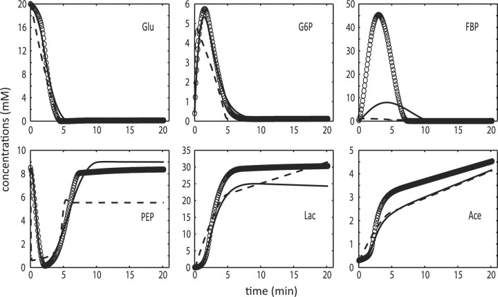
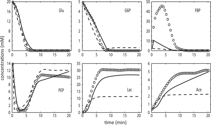
Table 3 reports the parameter estimation results using the ODE decomposition and the two-phase iterative method. Compared with the results from the ODE decomposition (Figure 5 and Table 3), the proposed method gave better concentration and slope fitting at roughly three times lower computational cost. In addition, the parameter errors from the two-phase method, though large, were comparably lower. Even with the full measurements, parameter identifiability issue has been shown to exist in this system (Srinath and Gunawan, 2010).

Table 3.

Parameter estimation of the L.lactis metabolic model

	ODE decomposition		Two-phase estimation
	w/o noise	Filtered data	w/o noise	Filtered data
Computational time (s)	79772.3	81858.8	24838.9	27325.2
Number of stiff ODE simulations	875	1023	316	368
Average parameter error (%)	243.90	–	97.29	–
Slope error (1/Na)	77.350	27090.2	2.3240	1.4910
Concentration error (1/Na)	24.777	288.71	24.784	24.573

^aN is the number of time points in each metabolic profile.

Fig. 5.

Metabolic profiles in the L.lactis glycolytic pathway: in silico data (open circles), ODE decomposition (dashed line), and two-phase iterative estimation (solid line).

Finally, the two-phase iterative estimation and the ODE decomposition were applied to published smoothen NMR data using automated smoother (Vilela et al., 2007), again without X₃ The estimation results are also summarized in Table 3 and illustrated in Figure 6. As before, the proposed method gave markedly improved concentration and slope data fitting in shorter amount of time than the ODE decomposition method.

Fig. 6.

Metabolic profiles in the L.lactis glycolytic pathway: smoothen data (open circles), ODE decomposition (dashed line), and two-phase iterative estimation (solid line).

4 DISCUSSION

The proposed iterative parameter estimation method builds on the strengths of the decoupling method and the ODE decomposition method. By decoupling the ODEs, this method is significantly faster than other methods that require integrating complete coupled ODEs at each objective function evaluation, while still giving good fit to measured concentration data. In addition, like the ODE decomposition method, the combined approach does not require complete measurements of all metabolites and has much reduced parameter search space. As shown in the applications to the two cases, the proposed method was superior to the two methods from which it was developed. When metabolite measurements were incompletely available, the decoupling method could not be applied. Compared with the ODE decomposition method, the proposed method gave more accurate parameter estimates and better data fit (slope and concentration) at a much lower computational cost. While the fit to missing concentration measurement had an offset, it is noteworthy that the dynamic trend can be captured.

The combination of slope and concentration fitting had also been used in several existing parameter estimation methods. For example, Wang and Liu had developed a method where kinetic parameters were estimated simultaneously by minimizing both slope and concentration errors using a multiobjective optimization framework (Wang and Liu, 2008). Similar to the two-phase method here, Gennemark and Wedelin had proposed a multi-step method, where a derivative method was used to obtain an initial, rough guess of model parameters, for subsequent minimization of concentration error (Gennemark and Wedelin, 2007). These two methods however assumed that all metabolite measurements are available. Notably, in the latter, the ODEs were also solved one at a time using single or multiple shooting methods, thereby decoupling the parameter estimation problem as in the ODE decomposition. The shooting method can in fact be used to substitute the role of ODE decomposition in the two-phase iterative estimation, giving an alternative method.

Another method extended a class of ODE solvers, called orthogonal collocation method, for estimating model parameters (Ramsay et al., 2007). In this case, the concentrations were approximated as a linear combination of basis functions, where the coefficients were treated as nuisance parameters. Model parameters were then simultaneously estimated by minimizing the approximation errors between the simulated concentration and the data, and between the time-derivative of concentration prediction and the right hand side of Equation (1). Despite the similarities, the proposed method differs from this and the above methods in the grouping parameters into two, those that are associated with measured variables and those with unmeasured concentrations. By doing so, the parameter estimation can be solved more efficiently (solving a few small parameter estimation problems is easier than solving the combined, simultaneous estimation). Also, in this case, when more metabolites are measured, the estimation naturally becomes faster, since more parameters will be estimated in the first, computationally efficient phase.

Although the proposed method performed better than the ODE decomposition in terms of data fitting (i.e. lower slope and concentration errors), many of the parameter estimates were far from the true values (see Supplementary Tables S1 and S3). This may not be surprising as that the estimation problems had assumed missing data for one metabolite. Nevertheless, even with complete data, parameter identifiability has been shown to be lacking in the estimation of kinetic parameters from time-series data and the severity of this problem can be assessed quantitatively (Raue et al., 2009; Srinath and Gunawan, 2010).

Related to the identifiability issue, the kinetic information contained in different metabolites are not equal. The expected degradation in the accuracy of the parameter estimates from missing data depends on the degree of connectivity of the missing metabolite in two ways. The kinetic information (i.e. rate of change) of a metabolite is partially contained in the downstream and upstream metabolites in the metabolic network. The higher the degree of connectivity, by stoichiometry, of a missing metabolite, the more can the missing flux information be extracted from the available data. While this missing flux can be determined, the (initial) concentration of the unmeasured metabolite however is still lost. Thus, it is possible to capture the trend of the missing profiles, but not the concentration values, giving an offset between the simulated and true concentrations, as seen in the first and to some degree in the second example above.

However, when considering regulatory connectivity, the concentration of metabolite(s) is important. Here, the loss of concentration data of an important, highly connected regulatory metabolite will lead to a significant loss of information that cannot be easily recovered. In the first example, the loss of metabolite X₃ data represented the worst-case scenario, as this metabolite has a high regulatory connectivity and missing downstream metabolite data. On the other hand, if X₂ was not measured, the parameters can still be identified from other metabolites, since the set of p_u is null, i.e. the estimation can be done using only the decoupling method. Finally, an increase in the number of unmeasured metabolites will, in general, lead to lower overall kinetic information and poorer parameter estimates. In the first example, missing both X₂ and X₃ indeed gave less accurate parameter estimates, but the two-phase method still outperformed the ODE decomposition (Supplementary Tables S1, Supplementary Data and Supplementary Data).

For a given system, the computational requirement of the proposed method depends on several aspects, such as the number of measured and unmeasured metabolites, the number of parameters associated with measured and unmeasured metabolites, the convergence speed of the iterations, and as seen in the example, the noise in the data. In general, the higher the number of parameters involved in the first phase, the faster will the estimation finish. Unfortunately, the scalability of the method to larger systems is difficult to be determined as all of the factors mentioned above will interact. For example, the scaling will depend on the distribution of the additional parameters between the two phases as well as on the dynamics of the system (e.g. related to stiffness of the ODEs). In addition, the convergence will also play an important factor, but unfortunately, this is difficult to consider as the two phases have different objective functions.

Finally, while the applications considered in this article were taken from S-system models, the proposed iterative estimation is not limited to only BST models. The reason to consider these examples was that these models represent some of the most difficult parameter estimation problems due to the large number of parameters, stiff ODEs, and high degree of nonlinearity. The proposed method can also be applied to problems in which complete time-series data are available. In such a case, the parameters can be divided into two groups based on the level of difficulty in estimating them in each estimation phase. For example, for S-system models, the kinetic orders can be grouped together in the first phase (decoupling method), while the rate constants can be estimated in the second phase (ODE decomposition).

REFERENCES

- Chou I.C., Voit E.O. Recent developments in parameter estimation and structure identification of biochemical and genomic systems. Math. Biosci. 2009;219:57–83. doi: 10.1016/j.mbs.2009.03.002. [DOI] [PMC free article] [PubMed] [Google Scholar]
- Egea J.A., et al. Scatter search for chemical and bio-process optimization. J. Global Optim. 2007;37:481–503. [Google Scholar]
- Famili I., Palsson B.O. The convex basis of the left null space of the stoichiometric matrix leads to the definition of metabolically meaningful pools. Biophys. J. 2003;85:16–26. doi: 10.1016/S0006-3495(03)74450-6. [DOI] [PMC free article] [PubMed] [Google Scholar]
- Gennemark P., Wedelin D. Efficient algorithms for ordinary differential equation model identification of biological systems. IET Syst. Biol. 2007;1:120–129. doi: 10.1049/iet-syb:20050098. [DOI] [PubMed] [Google Scholar]
- Kimura S., et al. Inference of S-system models of genetic networks using a cooperative coevolutionary algorithm. Bioinformatics. 2005;21:1154–1163. doi: 10.1093/bioinformatics/bti071. [DOI] [PubMed] [Google Scholar]
- Maki Y., et al. Inference of genetic network using the expression profile time course data of mouse P19 cells. Genome Informatics. 2002;13:382–383. [Google Scholar]
- Marino S., Voit E.O. An automated procedure for the extraction of metabolic network information from time series data. J. Bioinform. Comput. Biol. 2006;4:665–691. doi: 10.1142/s0219720006002259. [DOI] [PubMed] [Google Scholar]
- Montgomery D.C., Runger G.C. Applied Statistics and Probability for Engineers. Hoboken, NJ: John Wiley & Sons Pte Ltd; 2007. [Google Scholar]
- Neves A.R., Santos H. Overview on sugar metabolism and its control in Lactococcus lactis - the input from in vivo NMR. FEMS Microbiol. Rev. 2005;29:531–554. doi: 10.1016/j.femsre.2005.04.005. [DOI] [PubMed] [Google Scholar]
- Ramos A., et al. Metabolism of lactic acid bacteria studied by nuclear magnetic resonance. Antonie Van Leeuwenhoek. 2002;82:249–261. [PubMed] [Google Scholar]
- Ramsay J.O., et al. Parameter estimation for differential equations: a generalized smoothing approach. J. Roy. Stat. Soc. B. 2007;69:741–770. [Google Scholar]
- Raue A., et al. Structural and practical identifiability analysis of partially observed dynamical models by exploiting the profile likelihood. Bioinformatics. 2009;25:1923–1929. doi: 10.1093/bioinformatics/btp358. [DOI] [PubMed] [Google Scholar]
- Rodriguez-Fernandez M., et al. Novel metaheuristic for parameter estimation in nonlinear dynamic biological systems. BMC Bioinformatics. 2006;7:483. doi: 10.1186/1471-2105-7-483. [DOI] [PMC free article] [PubMed] [Google Scholar]
- Savageau M.A. Biochemical systems analysis. I. Some mathematical properties of the rate law for the component enzymatic reactions. J. Theor. Biol. 1969;25:365–369. doi: 10.1016/s0022-5193(69)80026-3. [DOI] [PubMed] [Google Scholar]
- Savageau M.A. Biochemical systems analysis. II. The steady-state solutions for an n-pool system using a power-law approximation. J. Theor. Biol. 1969;25:370–379. doi: 10.1016/s0022-5193(69)80027-5. [DOI] [PubMed] [Google Scholar]
- Savageau M.A., Voit E.O. Power-law approach to modeling biological-systems. 1. Theory. J. Ferment. Technol. 1982;60:221–228. [Google Scholar]
- Sorribas A., Cascante M. Structure identifiability in metabolic pathways: parameter estimation in models based on the power-law formalism. Biochem. J. 1994;298(Pt 2):303–311. doi: 10.1042/bj2980303. [DOI] [PMC free article] [PubMed] [Google Scholar]
- Srinath S., Gunawan R. Parameter identifiability of power-law biochemical system models. J. Biotechnol. 2010;149:132–140. doi: 10.1016/j.jbiotec.2010.02.019. [DOI] [PubMed] [Google Scholar]
- Vilela M., et al. Automated smoother for the numerical decoupling of dynamics models. BMC Bioinformatics. 2007;8:305. doi: 10.1186/1471-2105-8-305. [DOI] [PMC free article] [PubMed] [Google Scholar]
- Vilela M., et al. Identification of neutral biochemical network models from time series data. BMC Syst. Biol. 2009;3:47. doi: 10.1186/1752-0509-3-47. [DOI] [PMC free article] [PubMed] [Google Scholar]
- Voit E.O. Computational Analysis of Biochemical Systems: A Practical Guide for Biochemists and Molecular Biologists. Cambridge, UK: Cambridge University; 2000. [Google Scholar]
- Voit E.O., Almeida J. Decoupling dynamical systems for pathway identification from metabolic profiles. Bioinformatics. 2004;20:1670–1681. doi: 10.1093/bioinformatics/bth140. [DOI] [PubMed] [Google Scholar]
- Voit E.O., Savageau M.A. Power-law approach to modeling biological-systems. 2. Application to ethanol-production. J. Ferment. Technol. 1982;60:229–232. [Google Scholar]
- Voit E.O., Savageau M.A. Power-law approach to modeling biological-systems. 3. Methods of analysis. J. Ferment. Technol. 1982;60:233–241. [Google Scholar]
- Wang F.S., Liu P.K. Inverse problems of biological systems using multi-objective optimization. J. Chin. Inst. Chem. Eng. 2008;39:399–406. [Google Scholar]
- Yao K.Z., et al. Modeling ethylene/butene copolymerization with multi-site catalysts: parameter estimability and experimental design. Polym. React. Eng. 2003;11:563–588. [Google Scholar]
Associated Data
This section collects any data citations, data availability statements, or supplementary materials included in this article.